An observer-based adaptive control design for the maglev system

Abstract

In this study, a nonlinear adaptive controller that can be used to control a magnetic levitation (maglev) is designed. The designed controller is equipped with a nonlinear velocity observer to provide the control without measuring velocity. Its capability to adaptively compensate all parametric uncertainties during the control process is one of the main advantages of this controller. Utilizing this capability, control of the maglev system can be realized without using any knowledge about system parameters. Due to the fast convergence capability of the designed observer and the desired model dependent structure of the adaptation rules, the proposed control design provides better performance than most of the robust and adaptive controllers that have been frequently used to control maglev system. The observer dynamics are analyzed via a Lyapunov–like preliminary analysis. Then, convergence of the observation and the tracking errors under the closed–loop operation and stability of the closed–loop error dynamics are proven via a Lyapunov–based stability analysis where the result obtained in the mentioned preliminary analysis is used. Performance of the designed observer–controller couple is demonstrated via experimental results. The efficiency of the designed controller is tested against a robust proportional–integral–derivative (PID) controller and an another Lyapunov–based nonlinear robust controller called as robust integral of sign of error (RISE) controller. Experimental results show that the designed controller performs the best tracking performance with the least control effort among these three controllers.

Keywords

Maglev system robust control adaptive control nonlinear control nonlinear observer Lyapunov

Introduction

Devices that can hold ferromagnetic materials in the desired position in the air by using electromagnetic force are called as magnetic levitation (maglev) systems. The electromagnetic force required for this process is provided by an electromagnetic field generated by maglev systems. The ability of the mentioned devices to move the ferromagnetic materials in free air ensures that these devices form the basis of many other technologies. This ability removes the friction problem, and as a result of this, it is able to minimize the material wear. Maglev systems that can be used as an active suspension system have greatly contributed to ground transportation systems (Goodall and Kortum, 1983; Rote and Cai, 2002). They were considered and used as the main basis of development of magnetic train technologies (Givoni, 2006; Lee et al., 2006). Moreover, maglev systems can be utilized in many other applications such as vibration isolation in sensitive devices, and high precision positioning of chip plates in photolithography (Eroglu and Ablay, 2016). The efficiency of the usage of maglev systems in the mentioned applications and more is directly related with the efficiency of the controller designed to provide the control on the unstable equilibrium points of the system. This subject makes these systems suitable for testing different types of linear and nonlinear control approaches. As a result of these, control design for the maglev systems has become an important and an attractive subject for the research area of control.

When the literature is reviewed it is seen that control design for the maglev and maglev–based systems is a long–standing and popular topic. In Matsumura and Yoshimoto (1986), an integral type control was designed to get the rotor of the magnetic bearing system to the desired point and maintain its position. In Cho et al. (1993), a comparative control study about the control of maglev system was presented. The comparison was experimentally realized between the sliding–mode controller (SMC) and a classical controller. Other SMC approaches used for the control of maglev and maglev–based systems were presented in Yeh et al. (1999), Hajjaji and Ouladsine (2001) and Lin et al. (2007). In Yeh et al. (1999), SMC approach was used for the control of a magnetic bearing system. In Hajjaji and Ouladsine (2001), asymptotic regulation of the maglev system was guaranteed via static and dynamic type SMCs while the friction force and the other uncertainties were compensated. Position tracking of the maglev system was provided via a radial basis function (RBF) network-based intelligent SMC in Lin et al. (2007). In Green and Craig (1998), experimental performances of robust, adaptive and nonlinear controllers on the control of maglev system were demonstrated. A self–tuning adaptive stabilizing controller was designed for the control of repulsive maglev guiding system in Chen et al. (2000). In the mentioned study, the stability of the overall system and regulating precision were provided via the designed controller without using the exact knowledge of various components.

Design and experimental verification of linear and nonlinear state-space controllers equipped with velocity observers are presented in Barie and Chiasson (2000). Both of the control designs presented in the mentioned study were based on linearized system models. In Yang et al. (2004), the position tracking problem of the maglev system was solved via a robust nonlinear control design. In the mentioned control design uncertainties of physical parameters and the modeling errors caused from these uncertainties were taken into account and the controller was designed by considering its robustness against them. In Lin et al. (2009), a proportional–integral–derivative (PID)–type SMC controller and the PID–type dynamic SMC controller were adopted for the control of maglev system. In Chen et al. (2009), another PID control approach was presented to cope with the unbalanced vibration problems of an active magnetic bearing system. The mentioned PID controller was equipped with a fuzzy gain tuning mechanism to increase its efficiency.

This topic has maintained its popularity over the last decade. In Baranowski and Piatek (2012), a laboratory maglev system was controlled via a PID–based control design. Different from the classical PID control applications, the mentioned PID controller was supported with a velocity observer and a nonlinear feedforward to improve the control quality and stable range of the motion. In Michail et al. (2012), control of an electromagnetic suspension system was provided via a combination of the linear quadratic Gaussian control, the fault tolerant control and the multiobjective optimization. In Wai et al. (2010), stabilization, balance and the propulsive positioning of a maglev transportation system were provided via a PID control based on real–time particle swarm optimization (PSO). Another combination of the PSO and the PID control approach is available in Lin et al. (2011). In the mentioned study the position tracking of the maglev system was ensured via an adaptive PID controller combined with a PSO method to obtain the optimal learning–rates of the adaptation rule. An adaptive control approach based on online algebraic estimation of the system parameters, linearization and generalized proportional integral control was proposed for the control of maglev system in Morales et al. (2010). In Yanga et al. (2011), position tracking of a maglev suspension system was provided via a nonlinear disturbance observer based nonlinear robust controller design while the exponential tracking control of the maglev system was provided via a robust nonlinear control design in Zhang et al. (2015). In Al-Araji (2016), a cognitive online auto–tune algorithm based on backstepping technique was utilized to develop a novel position–tracking control algorithm for a maglev system.

SMC approach has also preserved its popularity for the control of maglev system in the last decade. An application of an active magnetic bearing system used to levitate the elevation axis of an electro–optical sight mounted on a moving vehicle and controlled via the SMC by considering the robustness of this method against model uncertainties and its reducing capability on disturbance responses was described in Kang et al. (2010). Cascade structured SMC designs presented in Eroglu and Ablay (2016) and Ginoya et al. (2016) can be given as two of many SMC examples that can be found in the literature of maglev control systems in this process. In Tepljakov et al. (2018), control of the maglev system was ensured via the fractional–order PID control. In the mentioned study, model reference adaptive control was utilized to realize the fractional order PID control under the closed–loop operation and the PID controller was equipped with a disturbance rejection algorithm. An improved adaptive fuzzy backstepping controller that is able to control the maglev system in the presence of parametric and structural uncertainties was designed in Sadek et al. (2017). An integral joint structure based control strategy was proposed for stabilization of maglev train in Wang et al. (2018). A self–tuning robust integral of signum of error (RISE) based controller was designed and used in a cascade control system that was proposed for the control of maglev system in Bidikli and Bayrak (2018). An application of a robust control design based on approximate feedback linearization technique to an electromagnetic levitation system was presented in Oh and Choi (2018). In Adiguzel et al. (2018), an adaptive backstepping control design developed to compensate position tracking error of an iron ball in a maglev system was presented. A nonlinear state feedback controller design was realized in Khimani et al. (2018) to ensure high performance step response of maglev system. In Humaidi et al. (2018), performance comparison of linear and nonlinear active disturbance rejection controllers for control and disturbance rejection of maglev system was presented. A PID controller and an adaptive neural–fuzzy SMC were presented in Sun et al. (2019b) for the magnetic suspension control of a low–speed maglev train. In Sun et al. (2019a), an exponential reaching law based SMC supported with an RBF neural network estimator was designed for the control of maglev system. Another RBF network approximation based sliding mode adaptive controller design realized for maglev vehicles nonlinear suspension system was presented in Chen et al. (2019).

These examples can easily be increased when the popularity of the subject is considered. However, the studies mentioned in this section are sufficient to make some determinations about the control of maglev and maglev–based systems. When the studies given in this section are examined with many other studies available in this literature it can be observed that robust control approach has been frequently preferred for the control of these type of systems. Structure of robust controllers that does not need any information about the system model and its parameters is feasible to cope with parametric and structural uncertainties that are commonly encountered problems in the control of maglev systems. However, their high control effort requirement can be considered as their main disadvantage. Since this situation causes from the structure of the robust controllers that works according to the worst case scenario, it is an inevitable situation. Moreover, most of these type of designs need measurements of all states (i.e. position and velocity of the ferromagnetic material and the electromagnet current) to provide the control of these systems. The need for more measurements increases the possibility of encountering sensor precision problems. Controlling maglev systems becomes more compelling when the possible sensor precision problems are added to the aforementioned uncertainties. Therefore, in such a case, the need for control effort may become much higher. Adaptive control is an another commonly preferred method for the control of maglev systems. Adaptive controllers can be considered as feasible solutions for decreasing the control effort. Some of adaptive controllers can cope with high control effort requirement by compensating parametric and/or structural uncertainties while some of them were equipped with velocity observers to reduce the possible sensor precision problems by eliminating velocity measurement. However, when the literature is examined, it can be observed that most of the adaptive controllers equipped with velocity observers require partial knowledge about the system model, while most of the adaptive controllers that do not need any knowledge about the system model require the measurements of all states. Adaptive controllers that are completely independent from the system model and provide the control without using velocity measurement generally need additional parameter estimation tools to adaptively compensate the parametric uncertainties and/or separate velocity observer tools that were not designed as a part of control design to compensate the lack of velocity measurement. The control system may have a very complex structure when they are designed as separate tools and this is a disadvantage for the user.

Designing a nonlinear adaptive controller that can provide control of maglev system without using velocity measurement is the main purpose of this study. Designed controller compensates all parametric uncertainties while reaching this aim and it is equipped with a nonlinear velocity observer design to compensate the lack of velocity measurement. At this point it should be noted that the parameter estimations and velocity observation are not realized via additional tools, but rather designs included in the controller’s structure. Moreover, the designed controller provides better steady state performance than most of the robust and adaptive controllers available in the literature due to the fast convergence of the observer formulation and adaptations that are based on time–varying integral effect and the desired system model. The theoretical analysis of the designed controller is realized via Lyapunov–based arguments. Convergence of the observation and tracking errors under the closed–loop operations are shown mathematically in this analysis.

Maglev systems contain electrical and electromechanical subsystems in their structures. In the electrical subsystem the necessary electromagnet current that is utilized to get the ferromagnetic material to the desired position is generated via the input voltage. In the electromechanical subsystem, the ferromagnetic material is get to desired position via this electromagnet current. A cascade control structure based on the designed adaptive controller is proposed in this study by considering the mentioned structure. First, the necessary electromagnet current is determined by providing the controller of the electromechanical subsystem via the designed observer–controller couple and then the determined current value is obtained from the electrical subsystem via proportional–integral (PI) controller. The performance of the designed adaptive controller and the proposed control structure are demonstrated via experimental studies. Additionally, comparative experimental studies are presented to show the aforementioned advantages of the designed controller.

The rest of the paper is organized in the following manner. The first section after the Introduction section describes the dynamical model of the maglev system along with its properties. The section about system model is followed by a section where the control design and related analysis are presented in a detailed manner. Finally, the paper is concluded by giving experimental results and concluding remarks, respectively.

Dynamic model of the Maglev system

The maglev system whose schematic is given in Figure 1 consists of two subsystems. One of these subsystems is called as an electrical subsystem. This subsystem is structured as a series resistor–inductor circuit that generates the electromagnet current from the input voltage. The relation between the electromagnet current and the ball’s position can be examined by considering other subsystem called as an electromechanical subsystem. Mathematical model of the maglev system can be examined by considering mathematical models of the mentioned subsystems. These mathematical models are tried to be examined in a detailed manner in this section.

Dynamic model of the electrical subsystem

Electrical subsystem of the maglev system is constructed by connecting a resistor, a coil having a variable and iron ball’s position dependent inductance value, and an alternative current voltage source in series. The position of the iron ball and the inductance value are represented by $x (t)$ and $L (x) \in R$ , respectively in Figure 1. Inductance value of the electromagnet varies between the value of the inductance in the absence of the iron ball and value of the inductance when the iron ball is in contact with the electromagnet. These values are denoted by $L_{1}$ and $L_{2} ≜ L_{0} + L_{1} \in R$ , respectively. The inductance value between these limits is determined according to the position of the iron ball with the formula given as Eroglu and Ablay (2016)

L = L_{1} + \frac{k}{x}

(1)

where $k \in R$ is an electromechanical constant defined as

k ≜ x_{0} L_{0}

(2)

where an additive constant inductance value that is effective on the inductance value around the operating point $x_{0} \in R$ is denoted by $L_{0} \in R$ Eroglu and Ablay (2016). By considering its structure and the aforementioned relations the dynamic model of the electrical subsystem is given as

V = I (R + R_{s}) + L \overset{\cdot}{I} + I \overset{\cdot}{L}

(3)

where $V \in R$ denotes the input voltage while the electromagnet current is represented by $I \in R$ . Resistor values of the electromagnet and the position sensor are denoted by $R$ and $R_{s} \in R$ , respectively. The dynamic model of the electrical subsystem can be rearranged as

\overset{\cdot}{I} = \frac{1}{L} V - \frac{(R + R_{s})}{L} I + \frac{k}{L} \frac{\overset{\cdot}{x}}{x^{2}} I .

(4)

where (1) and (3) are utilized.

Dynamic model of the electromechanical subsystem

Force equations of the free–body diagram of the iron ball shown in Figure 1 are examined to obtain the mathematical model of the electromechanical subsystem. In the mentioned diagram, there are two forces namely as electromagnet and gravitational forces that affect the iron ball in the opposite directions. In Figure 1, $F_{c} (t) \in R$ is used to represent the electromagnet force while the gravitational force is represented by $F_{g} (t) \in R$ . During the levitation process, the electromagnet force is provided by the electromagnetic field and expressed as

F_{c} = - \frac{I^{2}}{2} \frac{dL}{dx}

(5)

while the gravitational force that causes from the mass of the iron ball expressed as

F_{g} = Mg

(6)

where $M \in R$ denotes the mass of the iron ball and the acceleration due to gravity is represented by $g \in R$ . After that point the equivalent force that is effective on the ball can be obtained via Newton’s second law as

F = F_{c} - F_{g} = \frac{k}{2} {(\frac{I}{x^{2}})}^{2} - Mg

(7)

where (1), (5) and (6) are utilized. The final form of the model can be arranged as

m (x) \overset{\cdot\cdot}{x} + f (x) = u

(8)

where $m (x) ≜ \frac{2 M x^{2}}{k}$ , $f (x) ≜ \frac{2 Mg x^{2}}{k}$ , $u ≜ I^{2}$ and (7) is utilized.

Remark 1: In some of the studies about control of maglev systems control designs were based on the nonlinear state space model of this system given as

{\overset{\cdot}{x}}_{v} = f_{v_{1}} (x, \overset{\cdot}{x}, I, V)

(9)

y = f_{v_{2}} (x, I)

(10)

where $x_{v} \in R^{3}$ denotes the vector of system states defined as $x_{v} ≜ {[\begin{matrix} x & \overset{\cdot}{x} & I \end{matrix}]}^{T}$ and $y \in R^{2}$ denotes the vector of the output of the system for the case that velocity of the system is unmeasurable. Vector of functions $f_{v_{1}} (x, \overset{\cdot}{x}, I, V) \in R^{3}$ and $f_{v_{2}} \in R^{2}$ are defined as

f_{v_{1}} ≜ {[\begin{matrix} \overset{\cdot}{x} & \frac{k}{2 M x^{2}} I^{2} - g & \frac{1}{L} V - \frac{(R + R_{s})}{L} I + \frac{k}{L} \frac{\overset{\cdot}{x}}{x^{2}} I \end{matrix}]}^{T}

(11)

f_{v_{2}} ≜ {[\begin{matrix} x & I \end{matrix}]}^{T} .

(12)

Providing the position control of an iron ball just by designing the input voltage by considering the structure of the model in (9)–(12) was the main aim for the mentioned studies. However, in this study the control inputs of electrical and electromechanical subsystems are designed separately. Then, the mentioned aim is reached by combining these designs in a cascade control structure. Considering this situation, dynamic models of electrical and electromechanical subsystems are presented separately in this section.

As it can be seen in Figure 1, the iron ball moves in a limited space. This situation makes the position of the iron ball $x$ a bounded variable. Moreover, since the system is physically prevented from $x = 0$ position, electromagnet force becomes a bounded variable. This situation guarantees the boundedness of the velocity of the iron ball. Due to these basic facts arising from the nature of the maglev system, the following properties are satisfied. At this point it should be stated that since the mentioned situations are valid for all maglev systems, the given properties are also valid for all maglev systems. Owing to this fact the control design that will be presented in the following sections and will be based on these properties can be generalized for the control of maglev systems.

Property 1: The following lower and upper bounds can be provided for $m (\cdot)$ by utilizing the lower and upper boundedness of the position of the iron ball

m_{ℓ} \leq m (\cdot) \leq m_{u}

(13)

\frac{1}{m_{u}} \leq \frac{1}{m (\cdot)} \leq \frac{1}{m_{ℓ}}

(14)

and the following upper bound can be obtained for its time derivative by utilizing the upper boundedness of position and velocity of the iron ball

\overset{\cdot}{m} (\cdot) \leq m_{d_{u}}

(15)

where $m_{ℓ}$ , $m_{u}$ and $m_{d_{u}} \in R^{+}$ represent the positive constant bounding terms.

Property 2: For the absolute value of some of the functions of terms $m (\cdot)$ and $f (\cdot)$ , the following upper bounds can be satisfied

| m (φ) - m (ϕ) | \leq ξ_{m_{1}} | φ - ϕ |

(16)

| \frac{1}{m (φ)} - \frac{1}{m (ϕ)} | \leq ξ_{m_{2}} | φ - ϕ |

(17)

| f (φ) - f (ϕ) | \leq ξ_{f} | φ - ϕ |

(18)

$\forall φ$ and $\forall ϕ \in R$ that provide bounds of the position of the iron ball. In (16)–(18), $ξ_{m_{1}}$ , $ξ_{m_{2}}$ and $ξ_{f} \in R^{+}$ denote positive bounding constants.

In addition to these properties, the following property that is valid for the system model in (8) will later be utilized for the control design

Property 3: The final form of the dynamic model of an electromechanical subsystem in (8) can be expressed as a multiplication of a regression vector denoted by $y (x, \overset{\cdot\cdot}{x}) \in R^{2}$ and another vector that contains the constant system parameters and denoted by $θ \in R^{2}$ as

y (x, \overset{\cdot\cdot}{x}) θ ≜ m (x) \overset{\cdot\cdot}{x} + f (x)

(19)

where $y (x, \overset{\cdot\cdot}{x}) ≜ [\begin{matrix} x^{2} \overset{\cdot\cdot}{x} & x^{2} \end{matrix}]$ and $θ ≜ {[\begin{matrix} \frac{2 M}{k} & \frac{2 Mg}{k} \end{matrix}]}^{T}$ . The expression of the dynamic model in (19) can be written in terms of the desired position and its time derivatives as

y_{d} (x_{d}, {\overset{\cdot\cdot}{x}}_{d}) θ ≜ m (x_{d}) {\overset{\cdot\cdot}{x}}_{d} + f (x_{d})

(20)

where $y_{d} (x_{d}, {\overset{\cdot\cdot}{x}}_{d}) \in R^{2}$ denotes a function of the desired position $x_{d} (t) \in R$ and its second time derivative ${\overset{\cdot\cdot}{x}}_{d} (t) \in R$ . At this point it should be noted that, this function is obtained by writing $x_{d} (t)$ and ${\overset{\cdot\cdot}{x}}_{d} (t)$ instead of $x (t)$ and $\overset{\cdot\cdot}{x} (t)$ in the definition of $y (\cdot)$ .

Control design and analysis

Controlling the position of the iron ball via applied input voltage is the general control approach for the maglev system. It can be observed from the previous section that the necessary electromagnet current is provided via the input voltage while the position of the ball can be brought to desired level via this current. The control process is realized in two steps in this study by considering these issues. First, the necessary electromagnet current is determined from the control input of the electromechanical subsystem as it is defined in (8). To realize this, a nonlinear adaptive control approach that only needs the position measurement to provide the control is designed and applied to this part. This controller is combined with a nonlinear velocity observer design to compensate the lack of velocity measurement. Then, the necessary input voltage is obtained from the electrical subsystem via a PI controller. The current value obtained from the control of electromechanical subsystem is used as the desired current during the control process of the electrical subsystem.

Remark 2: At this point it should be noted that these type of cascade systems were successfully used in Eroglu and Ablay (2016) and Bidikli and Bayrak (2018) for the control of maglev system. In both of the mentioned studies different type of controllers designed for the control of electromechanical subsystem were combined with PI controller. In this study, PI controller is preferred for the control of electrical subsystem by inspiring from Eroglu and Ablay (2016) and Bidikli and Bayrak (2018).

Block diagram of the control process that is examined in a detailed manner in this section is shown in Figure 2. At this point it should be stated that equations and variables shown in Figure 2 that have not been defined so far are examined in a detailed manner in the following subsections.

Control of the electromechanical subsystem

Designing a controller that provides a satisfactory tracking performance between the position $x$ and the desired position $x_{d}$ is the main purpose of this part. To formulate this problem, the tracking error $e (t) \in R$ is defined as

e ≜ x_{d} - x

(21)

where the desired position $x_{d}$ and its first and second order time derivatives are bounded (i.e. $x_{d}$ , ${\overset{\cdot}{x}}_{d}$ and ${\overset{\cdot\cdot}{x}}_{d} \in L_{\infty}$ ). Velocity observation error $\overset{\cdot}{\tilde{x}} (t) \in R$ and position observation error $\tilde{x} (t) \in R$ that will later be utilized in the observer design are defined as

\overset{\cdot}{\tilde{x}} ≜ \overset{\cdot}{x} - \overset{\cdot}{\hat{x}}

(22)

\tilde{x} ≜ x - \hat{x}

(23)

where the observed position and velocity are denoted by $\hat{x} (t)$ and $\overset{\cdot}{\hat{x}} (t) \in R$ , respectively. The difference between the vector of constant system parameters $θ$ and their estimations $\hat{θ} \in R^{2}$ is defined as parameter estimation error. This error is denoted by $\tilde{θ} \in R^{2}$ and mathematically expressed as

\tilde{θ} ≜ θ - \hat{θ} .

(24)

The following auxiliary error terms are also defined to simplify the subsequent stability analysis by eliminating higher order time derivatives from it

r ≜ \overset{\cdot}{e} + α e

(25)

s ≜ \overset{\cdot}{\tilde{x}} + α \tilde{x}

(26)

where $α \in R^{+}$ is a positive constant gain.

Observer-based adaptive control design

The velocity observer is designed as follows

\overset{\cdot}{\hat{x}} = p + k_{0} \tilde{x} - k_{c} e

(27)

where the update rule for the auxiliary signal denoted by $p \in R$ is given as

\overset{\cdot}{p} = k_{1} sgn (\tilde{x}) + k_{2} \tilde{x} - α k_{c} e

(28)

where $k_{0}$ , $k_{c}$ , $k_{1}$ and $k_{2} \in R^{+}$ are positive constant observer gains and $sgn (\cdot) \in R$ denotes the signum function. The designed observer is used as a part of control input to provide the control of the maglev system and this design is given as

u = y_{d} \hat{θ} + k_{p} e + α k_{c} (x_{d} - \hat{x}) + k_{c} ({\overset{\cdot}{x}}_{d} - \overset{\cdot}{\hat{x}})

(29)

where $k_{p} \in R^{+}$ denotes the positive constant control gain.

The following expression can be obtained by utilizing (21) and (23)

x_{d} - \hat{x} = e + \tilde{x} .

(30)

The control design in (29) can be rearranged as follows by substituting (30) and its first time derivative into it

u = y_{d} \hat{θ} + k_{p} e + k_{c} (r + s)

(31)

where (25) and (26) are utilized. In (8), the control input is defined as the square of the electromagnet current. According to this definition the electromagnet current’s value becomes a complex number for the negative values of the control input. The following saturation function can be applied on control input to avoid this situation and to guarantee the nonnegativeness of the control input

u (t) = {\begin{matrix} u (t), & u (t) \geq 0 \\ 0, & u (t) < 0 \end{matrix} .

(32)

Remark 3: None of the experiments performed for different scenarios on the experimental system used in this study required the saturation function given in (32). In all of the experiments, the control input was not negative, and as a result, real current values were obtained. However, from the mathematical definition of the control input it is clear that the nonnegativeness of the control input must be guaranteed. The saturation function in (32) is given by considering this requirement and by applying it, the designed controller can be used for the control of maglev and maglev–based systems without having to worry about the possibility that the control input is negative.

Preliminary analysis for the observer dynamics

In this section observer error dynamics are analyzed via a Lyapunov–like analysis. The result obtained from this analysis will be used in the Lyapunov–based stability analysis of the closed–loop error dynamics of the designed observer–controller couple. The time derivative of (22) is rearranged as

\overset{\cdot\cdot}{\tilde{x}} = N_{0} - k_{1} sgn (\tilde{x}) - k_{2} \tilde{x} - k_{0} \overset{\cdot}{\tilde{x}} + k_{c} r

(33)

where (8) and (25) are utilized. The auxiliary term denoted by $N_{0} \in R$ is defined as

N_{0} ≜ \frac{1}{m} (u - f) .

(34)

This auxiliary term can be partitioned as a sum of two newly defined auxiliary terms by substituting (31) into (34)

N_{0} ≜ N_{d} + N_{b}

(35)

where (20) and (24) are utilized and the auxiliary terms $N_{d} (t)$ and $N_{b} (t) \in R$ are defined as

N_{d} ≜ - \frac{1}{m (x_{d})} y_{d} \tilde{θ} + {\overset{\cdot\cdot}{x}}_{d}

(36)

\begin{matrix} N_{b} ≜ [\frac{1}{m (x_{d})} - \frac{1}{m (x)}] (y_{d} \tilde{θ} - m (x_{d}) {\overset{\cdot\cdot}{x}}_{d}) \\ + \frac{1}{m (x)} [k_{p} e + k_{c} (r + s) + f (x_{d}) - f (x)] . \end{matrix}

(37)

At this point it should be noted that the boundedness of $N_{d} (t)$ and ${\overset{\cdot}{N}}_{d} (t)$ can be guaranteed via the boundedness of the desired trajectory. Moreover, the following theorem is presented to show the boundedness of $N_{b} (t)$ .

Theorem 1: The absolute value $N_{b} (t)$ can be upper bounded as follows based on the definition given in (37)

| N_{b} | \leq ρ_{01} | e | + ρ_{02} {| r | + | s |}

(38)

where $ρ_{01}$ and $ρ_{02} \in R^{+}$ denotes the positive bounding constants whose numerical values are known.

Proof: See Appendix 1 for the proof.

The preliminary analysis can be continued by rearranging the time derivative of (26) by utilizing (33) and (35) as

\overset{\cdot}{s} = N_{d} + N_{b} - k_{1} sgn (\tilde{x}) - k_{2} \tilde{x} - k_{0} \overset{\cdot}{\tilde{x}} + k_{c} r + α \overset{\cdot}{\tilde{x}} .

(39)

For the selection of the observer gains given as

k_{2} = α (k_{0} - α)

(40)

the expression given in (39) can be rearranged as

\overset{\cdot}{s} = N_{d} + N_{b} - k_{1} sgn (\tilde{x}) - \frac{k_{2}}{α} s + k_{c} r

(41)

where (25) is utilized. The following lemma should be stated for the completeness of this analysis.

Lemma 1: The nonnegativeness of an auxiliary term $P (t) \in R$ defined as

P ≜ ξ_{p} - \int_{t_{0}}^{t} ω (σ) d σ

(42)

can be guaranteed via definitions of $ω (t)$ and $ξ_{p} \in R$ given as

ω ≜ s (N_{d} - k_{1} sgn (\tilde{x}))

(43)

ξ_{p} ≜ k_{1} | \tilde{x} (t_{0}) | - \tilde{x} (t_{0}) N_{d} (t_{0})

(44)

and the selection of $k_{1}$ given as

k_{1} \geq | N_{d} (t) | + \frac{1}{α} | {\overset{\cdot}{N}}_{d} (t) | .

(45)

Proof: See Appendix 2 for the proof.

The following nonnegative Lyapunov–like function can be defined to complete the Lyapunov–like analysis

V_{0} ≜ \frac{1}{2} s^{2} + P .

(46)

The time derivative of $V_{0} (t) \in R$ can be obtained as follows by utilizing (41) and the time derivative of (42)

{\overset{\cdot}{V}}_{0} = s (- \frac{1}{α} k_{2} s + N_{b} + k_{c} r) .

(47)

Error system development

The time derivative of (25) is multiplied with $m$ and (8) and (21) are utilized in the resulting equation to obtain the open–loop error dynamics given as

m \overset{\cdot}{r} = y_{s} θ - u

(48)

where $y_{s} (t) \in R^{2}$ denotes the regressor vector defined as $y_{s} (t) ≜ [\begin{matrix} x^{2} ({\overset{\cdot\cdot}{x}}_{d} + α \overset{\cdot}{e}) & x^{2} \end{matrix}]$ . The term $y_{s} θ$ is obtained as

y_{s} θ = m ({\overset{\cdot\cdot}{x}}_{d} + α \overset{\cdot}{e}) + f .

(49)

The closed–loop error dynamics can be obtained as follows by substituting (31) into the open–loop error dynamics

m \overset{\cdot}{r} = χ - k_{p} e - k_{c} (r + s) + y_{d} \tilde{θ}

(50)

where an error–like auxiliary term denoted by $χ \in R$ is defined as

χ ≜ (y_{s} - y_{d}) θ .

(51)

At this point the boundedness of $χ$ should be given via the following theorem by considering the following parts of the analysis.

Theorem 2: The upper bound of the absolute value of the auxiliary term $χ (t)$ can be obtained as

| χ | \leq ρ_{1} | e | + ρ_{2} | r |

(52)

where $ρ_{1}$ and $ρ_{2} \in R^{+}$ are known positive bounding constants.

Proof: See Appendix 3 for the proof.

After that point Lyapunov–based stability analysis can be proceeded to show the convergence of the observation and the tracking errors under the closed–loop operation and to prove the stability of the closed–loop error dynamics.

Stability analysis

Theorem 3: The semi–global asymptotic stability of the closed–loop system that can be mathematically expressed as $| e (t) |, | \overset{\cdot}{\tilde{x}} (t) | \to 0 as t \to \infty$ can be ensured via the velocity observer design in (27) and (28) and the control design in (29) as long as the following selection criteria are provided for the constant gains

α k_{p} \geq 1

(53)

k_{c} = 1 + ρ_{2} + k_{n} ρ_{1}^{2} + \frac{1}{2} m_{d_{u}}

(54)

k_{2} = α [1 + ρ_{02} + k_{n} (ρ_{01}^{2} + ρ_{02}^{2})]

(55)

where $m_{d_{u}}$ was introduced in (15), $ρ_{01}$ and $ρ_{02}$ were introduced in (38) and the other constant gains $ρ_{1}$ and $ρ_{2}$ were introduced in (52). In (54) and (55), $k_{n} \in R^{+}$ is an another positive constant damping gain selected to satisfy $k_{n} > \frac{1}{2}$ .

Remark 4: Selection criteria about observer and controller gains in (40), (54) and (55) are necessary to reach the semi–global asymptotic stability of the closed–loop system, mathematically. They can be seen as restricted criteria for the selection of gains that should be adjusted by the user. However, from these equations it can be seen that the selection in (54) and (55) are directly related with $k_{c}$ and $k_{2}$ while the other selection in (40) is given as a relationship between $k_{0}$ and $k_{2}$ . Since the selection criteria of $k_{c}$ and $k_{2}$ are based on constants that can be selected arbitrarily, adjusting these gains via trial–and–error method to provide the tracking control efficiently and then selecting $k_{0}$ according to the value of $k_{2}$ is the most feasible way.

Proof: To propose a nonnegative Lyapunov function candidate, firstly nonnegative functions specified for tracking error $e$ , auxiliary error $r$ and parameter estimation error $\tilde{θ}$ are proposed and analyzed. Then, the nonnegative Lyapunov function candidate is proposed by summing them with $V_{0}$ defined in (46).

The first nonnegative function specified for the tracking error and denoted by $V_{1} (e) \in R$ is defined as

V_{1} ≜ \frac{1}{2} e^{2} .

(56)

The final form of the time derivative of the above function can be obtained as

{\overset{\cdot}{V}}_{1} = e (r - α e)

(57)

where (25) is utilized.

Other nonnegative function specified for the auxiliary error $r$ and denoted by $V_{2} (r) \in R$ is defined as

V_{2} ≜ \frac{1}{2} m r^{2} .

(58)

The final form of the time derivative of the above function can be obtained as

{\overset{\cdot}{V}}_{2} = r [χ - k_{p} e - k_{c} (r + s) + y_{d} \tilde{θ}]

(59)

where (50) is utilized.

The last nonnegative function specified for the parameter estimation error $\tilde{θ}$ and denoted by $V_{3} (\tilde{θ}) \in R$ is defined as

V_{3} ≜ \frac{1}{2 γ} {\tilde{θ}}^{T} \tilde{θ} .

(60)

where $γ \in R^{+}$ denotes the positive constant adaptation gain. The final form of the time derivative of the above function can be obtained as

{\overset{\cdot}{V}}_{3} = - \frac{1}{γ} {\tilde{θ}}^{T} \overset{\cdot}{\hat{θ}}

(61)

where (24) is utilized.

The nonnegative Lyapunov function candidate denoted by $V_{1} (z) \in R$ is defined as

V_{f} ≜ V_{0} + V_{1} + V_{2} + V_{3}

(62)

where $z (t) \in R^{6}$ is defined as

z ≜ {⌈ \begin{matrix} \sqrt{P} & s & r & e & {\tilde{θ}}^{T} \end{matrix} ⌉}^{T} .

(63)

The time derivative of (62) is obtained as

\begin{matrix} {\overset{\cdot}{V}}_{f} = s (- \frac{1}{α} k_{2} s + N_{b} + k_{c} r) + e (r - α e) \\ + r [χ - k_{p} e - k_{c} (r + s)] + {\tilde{θ}}^{T} (y_{d}^{T} r - \frac{1}{γ} \overset{\cdot}{\hat{θ}}) \end{matrix}

(64)

where (47), (57), (59) and (61) are utilized. When (64) is considered with the mathematical analysis that have been realized up to now, it can be seen that an upper bound can be proposed for ${\overset{\cdot}{V}}_{f}$ as long as the last term (i.e. the term given as ${\tilde{θ}}^{T} (y_{d}^{T} r - \frac{1}{γ} \overset{\cdot}{\hat{θ}})$ ) is eliminated. To continue this analysis by proposing an upper bound for the Lyapunov function candidate the parameter estimation vector is generated according to the following rule

\hat{θ} = γ (y_{d}^{T} e - \int_{t_{0}}^{t} \frac{d}{d σ} {y_{d}^{T} (σ)} e (σ) d σ + α \int_{t_{0}}^{t} y_{d}^{T} (σ) e (σ) d σ) .

(65)

Remark 5: Although it was not needed in many different experiments realized for this study, if there is a concern about the boundedness of (65) the given rule can be used as

\hat{θ} = Proj {γ (y_{d}^{T} e - \int_{t_{0}}^{t} \frac{d}{d σ} {y_{d}^{T} (σ)} e (σ) d σ + α \int_{t_{0}}^{t} y_{d}^{T} (σ) e (σ) d σ)} .

(66)

where $Proj (\cdot)$ denotes the standard projection operator.

Remark 6: At this point it should be noted that the parameter estimation rule given in (65) is not used to determine the exact numerical values of uncertain elements of $θ$ . Similar to most of other Lyapunov–based robust adaptive control designs this rule is designed as an adaptive compensation of uncertain terms. Uncertain elements of $θ$ can be adaptively compensated via finite numerical values generated according to (65) during the control process. The final numerical values of the estimations and error between the real parameters and estimations are not crucial as long as estimations change in a finite interval and it is theoretically proven that semi–global asymptotic stability of the closed–loop system is ensured when the estimation rule is designed as in (65).

Remark 7: From the definition of $θ$ in (19) it is seen that it contains almost the same two elements. However, since the terms corresponding these terms in the regression vector are different, a two–element parameter estimation rule must be developed in accordance with the structure of the designed controller.

After substituting the time derivative of (65) into (64), (64) can be rearranged as

{\overset{\cdot}{V}}_{f} = s (- \frac{1}{α} k_{2} s + N_{b} + k_{c} r) + e (r - α e) + r [χ - k_{p} e - k_{c} (r + s)] .

(67)

The upper bound of (67) can be obtained as follows after (53)–(55) are utilized

\begin{matrix} {\overset{\cdot}{V}}_{f} \leq - α k_{p} {| e |}^{2} - {| r |}^{2} - {| s |}^{2} + [ρ_{01} | e | | s | - k_{n} ρ_{01}^{2} {| s |}^{2}] \\ + [ρ_{02} | r | | s | - k_{n} ρ_{02}^{2} {| s |}^{2}] + [ρ_{1} | e | | r | - k_{n} ρ_{1}^{2} {| r |}^{2}] . \end{matrix}

(68)

The above inequality can be rearranged as follows after the terms inside the parenthesis are completed the squares

{\overset{\cdot}{V}}_{f} \leq - (α k_{p} - \frac{1}{2 k_{n}}) {| e |}^{2} - (1 - \frac{1}{4 k_{n}}) {| r |}^{2} - {| s |}^{2} .

(69)

To write (69) in a more compact form the vector of combined errors $c_{e} (t) \in R^{3}$ is defined as

c_{e} ≜ {[\begin{matrix} s & r & e \end{matrix}]}^{T}

(70)

and the upper bound of the time derivative of Lyapunov function candidate can be written in a more compact form by utilizing this definition as

{\overset{\cdot}{V}}_{f} \leq - (1 - \frac{1}{2 k_{n}}) ‖ c_{e} ‖^{2} .

(71)

From the upper bound of ${\overset{\cdot}{V}}_{f} (t)$ it is clearly seen that the nonnegativeness of the term given as $(1 - \frac{1}{2 k_{n}})$ must be determined to complete the analysis and it can be provided via the aforementioned selection of $k_{n}$ . The following reformulation can be proposed for (71) by considering this issue

{\overset{\cdot}{V}}_{f} \leq - β ‖ c_{e} ‖^{2}

(72)

where $β \in R^{+}$ denotes a positive constant that satisfies $0 < β \leq 1$ . From (62) and (72) it is seen that $V_{f} (t)$ is bounded.

The boundedness of $V_{f} (t)$ can be utilized to guarantee the boundedness of $z (t)$ and its elements (i.e. $z (t)$ , $e (t)$ , $r (t)$ , $s (t)$ , $P (t)$ , $\tilde{θ} (t) \in L_{\infty}$ ). The boundedness of all signals under the closed–loop operation can be shown via standard signal chasing arguments and from the boundedness of their time derivatives it can also be shown that $e (t)$ and $\overset{\cdot}{\tilde{x}} (t)$ are uniformly continuous signals. Moreover, from the integration of the both sides of (72), it can be shown that $c_{e} (t) \in L_{2}$ and consequently $e (t)$ , $\overset{\cdot}{\tilde{x}} (t) \in L_{2}$ . Finally, the asymptotic tracking result in Theorem 3 can be obtained via Barbalat’s Lemma (Khalil (2002).

Control of the electrical subsystem

Obtaining an efficient tracking between the current of the electromagnet and the desired current denoted by $I_{d} \in R$ is the main purpose of this part. As mentioned in previous sections, the desired current is determined according to the control input of the electromechanical subsystem. The tracking error between the mentioned current values $e_{I} (t) \in R$ is defined as

e_{I} ≜ I_{d} - I .

(73)

The auxiliary error term $r_{I} \in R$ is defined as

r_{I} ≜ {\overset{\cdot}{e}}_{I} + e_{I} .

(74)

PI control design

The input voltage that can be used as the control input to compensate the above tracking error is designed as

V = k_{p_{V}} e_{I} (t) + k_{i_{V}} \int_{t_{0}}^{t} e_{I} (σ) d σ

(75)

where the positive proportional and integral gains of PI controller are denoted by $k_{p_{V}}$ and $k_{i_{V}} \in R^{+}$ , respectively. The following saturation function determined according to the technical limitations of the experimental system is applied on the input voltage

V (t) = {\begin{matrix} V (t), & - 5 \leq V (t) \leq 5 \\ - 5, & V (t) < - 5 . \\ 5, & V (t) > 5 \end{matrix} .

(76)

Error system development

The open–loop error system of this part can be obtained as follows by multiplying the time derivative of (74) with $L$

L {\overset{\cdot}{r}}_{I} = (- k_{p_{V}} - R - R_{s} - \overset{\cdot}{L} + L) r + (k_{p_{V}} - k_{i_{V}} + R + R_{s} - L) e_{I} + N_{I}

(77)

where time derivative of (3), (73) and (74) are utilized and the auxiliary term $N_{I} (t) \in R$ is defined as

N_{I} ≜ L {\overset{\cdot\cdot}{I}}_{d} + (R + R_{s}) {\overset{\cdot}{I}}_{d} + \overset{\cdot}{L} ({\overset{\cdot}{I}}_{d} + I_{d}) .

(78)

Theorem 4: The boundedness of $I_{d}$ , its first and second order time derivatives, $x$ and $\overset{\cdot}{x}$ can be utilized to guarantee the boundedness of the auxiliary signal $N_{I}$ in the sense that

| N_{I} | \leq ρ_{I}

(79)

where $ρ_{I} \in R^{+}$ denotes the positive constant bounding term.

Stability analysis

Theorem 5: The control design in (75) provides local uniform ultimate boundedness of error terms in the sense that

‖ z_{I} ‖ \leq ε

(80)

where $ε \in R^{+}$ is a small positive constant and $z_{I} \in R^{2}$ is a vector of combined error terms defined as

z_{I} ≜ [\begin{matrix} e_{I} & r_{I} \end{matrix}]

(81)

as long as $k_{i_{V}}$ is selected according to

k_{i_{V}} > \frac{1}{2} + ρ_{L_{d}}

(82)

where $ρ_{L_{d}} \in R^{+}$ denotes a positive bounding constant of $\overset{\cdot}{L}$ (i.e. $| \overset{\cdot}{L} | \leq ρ_{L_{d}}$ ).

Proof: The nonnegative Lyapunov function candidate $V_{c} (z_{I}) \in R$ is defined as

V_{c} ≜ \frac{1}{2} (e_{I}^{2} + r_{I}^{2}) .

(83)

Time derivative of (83) is obtained as

\begin{matrix} {\overset{\cdot}{V}}_{c} = - e_{I}^{2} + (- k_{p_{V}} - R - R_{s} - \overset{\cdot}{L} + L) r_{I}^{2} + r_{I} N_{I} \\ + (k_{p_{V}} - k_{i_{V}} + R + R_{s} - L + 1) e_{I} r_{I} \end{matrix}

(84)

where time derivative of (73) and (77) are utilized. The following upper bound can be obtained for ${\overset{\cdot}{V}}_{c}$ when the fact $x_{1} x_{2} \leq \frac{1}{2} (x_{1}^{2} + x_{2}^{2})$ is utilized

\begin{matrix} {\overset{\cdot}{V}}_{c} \leq - [\frac{1}{2} (k_{p_{V}} + k_{i_{V}} + R + R_{s} - L + 2 \overset{\cdot}{L} - 2)] r_{I}^{2} \\ - [\frac{1}{2} (k_{p_{V}} - k_{i_{V}} + R + R_{s} - L + 1)] e_{I}^{2} + \frac{1}{2} ρ_{1}^{2} \end{matrix}

(85)

where (79) is utilized. The above inequality can be written in the following compact form

{\overset{\cdot}{V}}_{c} \leq - β_{I_{1}} ‖ z_{I} ‖ + β_{I_{2}}

(86)

when $k_{i_{V}}$ is selected to satisfy (82). Positive constant terms $β_{I_{1}}$ and $β_{I_{2}} \in R^{+}$ are defined as

\begin{matrix} β_{I_{1}} ≜ min {(k_{p_{V}} + k_{i_{V}} + R + R_{s} - L + 2 \overset{\cdot}{L} - 2), \\ (k_{p_{V}} - k_{i_{V}} + R + R_{s} - L + 1)} \end{matrix}

(87)

β_{I_{2}} ≜ \frac{1}{2} ρ_{I}^{2} .

(88)

The upper bound of ${\overset{\cdot}{V}}_{c}$ can be rearranged as follows for a region given as $D = {z_{I} \in R^{2} | η \leq ‖ z_{I} ‖}$ where $η ≜ \sqrt{\frac{1}{min {(k_{p_{V}} + k_{i_{V}} + R + R_{s} - L + 2 \overset{\cdot}{L} - 2), (k_{p_{V}} - k_{i_{V}} + R + R_{s} - L + 1)}} β_{I_{2}}}$

{\overset{\cdot}{V}}_{c} \leq - σ (‖ z_{I} ‖)

(89)

where $σ (‖ z_{I} ‖) \in R$ is a positive function. It is possible to make $η$ as small as possible by selecting the control gains large enough and owing to this, conditions given in Theorem 2.15 of Qu (1998) can be provided. The mentioned theorem can be used to show the local uniform ultimate boundedness of $e_{I}$ and $r_{I}$ . The boundedness of $e_{I}$ and $r_{I}$ can be used along with (74) to show the boundedness of ${\overset{\cdot}{e}}_{I}$ . Boundedness of ${\overset{\cdot}{e}}_{I}$ and boundedness of ${\overset{\cdot}{I}}_{d}$ show the boundedness of $\overset{\cdot}{I}$ when they are considered with (73). Boundedness of $I$ , $\overset{\cdot}{I}$ , $x$ , $\overset{\cdot}{x}$ can be utilized along with (4) to show that $V$ is also bounded under the closed–loop operation.

Experimental results

Maglev 33–210 experimental system produced by Feedback Instruments, shown in Figure 3, was used as an experimental setup. In this system, a ferromagnetic ball can be taken to the desired position via the current that is generated by the coil that acts as an electromagnet. The necessary measurements are obtained from the system via infrared sensors. Control input can be adjusted from the interface constructed in computer environment and can be applied to the system via a data acquisition card used to connect the experimental system to the computer.

Experiments were realized for constant and sinusoidal desired trajectories without changing the default settings of the experimental setup. In both of these studies, observer and control gains were adjusted to numerical values given as $α = 1$ , $k_{0} = 3.3$ , $k_{1} = 5.7$ , $k_{2} = 2.3$ , $k_{p} = 1.2$ , $k_{c} = 3.6$ and $γ = 1.9$ . Moreover, constant gains of the PI controller were adjusted as $k_{p_{V}} = 100$ and $k_{i_{V}} = 125$ .

The constant desired position was selected as

x_{d} (t) = 0.0055 m .

(90)

Actual and desired trajectories can be seen in Figure 4 while the tracking error and the control input can be seen in Figure 5 and Figure 6, respectively. The parameter estimations are given in Figure 7. Electromagnet’s current and the input voltage are demonstrated in Figure 8 and Figure 9, respectively. From Figure 4 and Figure 5, it is seen that the control objective was met.

The sinusoidal desired position was selected as

x_{d} (t) = 0.0035 \sin (π t) + 0.009 m .

(91)

Actual and desired trajectories can be seen in Figure 10 while the tracking error and the control input can be seen in Figure 11 and Figure 12, respectively. The parameter estimations are given in Figure 13. Moreover, electromagnet’s current and the input voltage are demonstrated in Figure 14 and Figure 15, respectively. From Figure 10 and Figure 11, it is seen that the control objective was met.

To demonstrate the efficiency of the designed controller against its two counterparts comparative experimental studies were realized. In the first part of these studies performance of the designed controller was compared with performance of the PID controller whose control input formulation is given as

u_{pid} = k_{p_{c 1}} e (t) + k_{i_{c 1}} \int_{t_{0}}^{t} e (σ) d σ + k_{d_{c 1}} \overset{\cdot}{e} (t)

(92)

where $k_{p_{c 1}}$ , $k_{i_{c 1}}$ and $k_{d_{c 1}} \in R^{+}$ denote the positive constant control gains of PID controller.

PID controller is one of the frequently used controllers to provide the control of maglev and maglev–based systems. This selection allows to compare the performance of the designed controller with a performance of the controller whose efficiency has been shown in many industrial and scientific applications. Observing the performance of the designed controller against a full state feedback counterpart is an another purpose of this comparison. Moreover, since PID controller is a robust controller its possible to compare the control effort requirement of the designed robust adaptive controller with a robust controller.

Then, performance of the designed controller was compared with the performance of its another Lyapunov–based nonlinear robust counterpart. The mentioned controller called as RISE controller is an another controller that has been widely used for the control of many different nonlinear systems in the research area of the control. The control input formulation of the RISE controller is given as Xian et al. (2004)

u_{RISE} = k_{c 2} [e_{2} (t) - e_{2} (t_{0}) + α_{2_{c 2}} \int_{t_{0}}^{t} e_{2} (σ) d σ] + β_{c 2} \int_{t_{0}}^{t} sgn (e_{2} (σ)) d σ

(93)

where $e_{2} (t) \in R$ denotes an auxiliary error signal defined as

e_{2} ≜ \overset{\cdot}{e} + α_{c 2} e .

(94)

and $k_{c 2}$ , $β_{c 2}$ , $α_{c 2}$ and $α_{2_{c 2}} \in R^{+}$ denote the positive constant control gains of RISE controller.

Observing the performance of the designed controller against another robust control structure is the main purpose of this part of the comparative experimental studies. Since the RISE controller is a nonlinear controller designed by utilizing Lyapunov–based arguments, this part of the comparative studies provides us a good opportunity to see the performance of the designed controller against an another controller that was constructed on similar bases. At this point it should be noted that all of these controllers were used for the control of electromechanical subsystem while they were cascaded with identically same PI controller structure for the control of electrical subsystem. Realizing the comparative studies under the similar conditions is the main purpose of this choice.

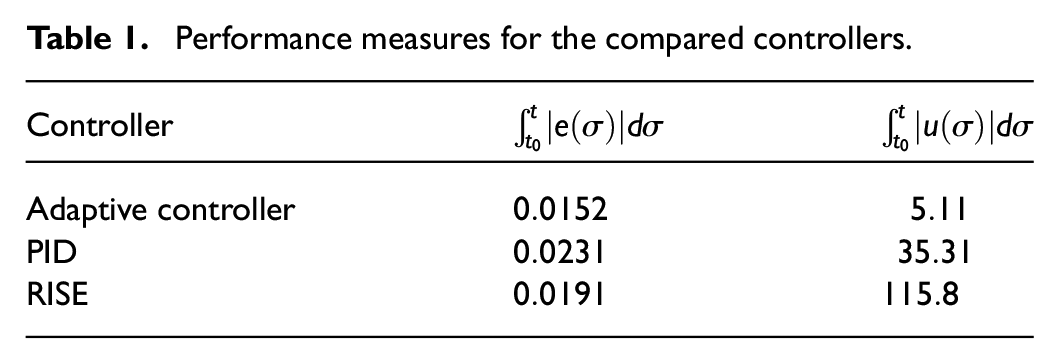
These experiments were realized for the sinusoidal desired position in (91). Control gains of the PID controller were adjusted via trial–and–error method until the best tracking performance was obtained. The final values of the control gains were obtained as $k_{p_{c 1}} = 55$ , $k_{i_{c 1}} = 97$ and $k_{d_{c 1}} = 2.5$ . Control gains of the RISE controller were adjusted via trial–and–error method until the best tracking performance was obtained. The final values of the control gains were obtained as $k_{c 2} = 0.05$ , $β_{c 2} = 0.6$ and $α_{c 2} = α_{2_{c 2}} = 1$ .

Tracking results and the control inputs for all controllers are shown in Figure 16 and Figure 17, respectively. The tracking performance and the control effort necessity are presented numerically in Table 1. To show the tracking performance numerically, area under the absolute value of the tracking error (i.e. $\int_{t_{0}}^{t} | e (σ) | d σ$ ) and to show the control effort necessity numerically, area under the absolute value of the control input (i.e. $\int_{t_{0}}^{t} | u (σ) | d σ$ ) were used as performance measures. From the presented results it can be clearly seen that the designed controller provides the best tracking performance with the least control effort necessity among these three controllers. It is an expected result that the designed controller needs less control effort than robust counterparts to provide the control when its adaptive structure is considered. The unexpected result is that the output feedback controller provides better tracking performance than the full state feedback counterparts. This result is rarely encountered in control applications. It may cause from bad measurement precision in the velocity measurement and can be interpreted as the designed controller would work more efficiently than the full state feedback counterparts if any problems about measurement precision are encountered. The positive effects of the fast convergence performance of the designed observer and the adaptation rules on the steady–state can be another possible reasons of the obtained results. Both of these situations can be considered as main advantages of the designed controller.

Table 1.

Performance measures for the compared controllers.

Controller	$\int_{t_{0}}^{t} \| e (σ) \| d σ$	$\int_{t_{0}}^{t} \| u (σ) \| d σ$
Adaptive controller	$0.0152$	$5.11$
PID	$0.0231$	$35.31$
RISE	$0.0191$	$115.8$

Conclusions

In this study, stabilization and control problem of a maglev system is solved by designing a robust adaptive controller. To get rid of the velocity measurement necessity in the designed controller, the control input is combined with a nonlinear velocity observer design that is able to compensate the lack of velocity measurement by estimating the velocity of the iron ball during its movement. A preliminary Lyapunov–like analysis presented in the study is utilized to theoretically analyze the behavior of the designed velocity observer and then the obtained result from this analysis is used in the stability analysis of the closed–loop error dynamics. The stability analysis of the closed–loop error dynamics of the designed observer–controller couple is realized via Lyapunov–based arguments. The electromagnet current that is necessary to get the ferromagnetic material to the desired position into the generated electromagnet field is obtained from the designed control input by applying it to the electromechanical subsystem. Then, the necessary input voltage is determined by providing the control of the electrical subsystem via a PI controller. The obtained current from the control of electromechanical system is used as the desired current for the control of electrical subsystem. Experimental studies that are supported with comparative results are presented in the study to demonstrate the performance and efficiency of the designed observer–controller couple.

Footnotes

Appendix 1: Proof of bound of absolute value of N b

The norm of $N_{b} (t)$ can be upper bounded as follows by considering the bounds of the dynamic terms in (13), (14), (16)–(18) with the definition of $N_{b} (t)$ in (37)

(95)

\begin{matrix} | N_{b} | \leq \frac{1}{m_{ℓ}} {ξ_{m_{2}} m_{u} m_{ℓ} | {\overset{\cdot\cdot}{x}}_{d} | + ξ_{m_{2}} m_{ℓ} | y_{d} \tilde{θ} | + ξ_{f} + k_{p}} | e | \\ + \frac{1}{m_{ℓ}} k_{c} {| r | + | s |} . \end{matrix}

From (95), it can be seen that (38) is provided for the following selections of $ρ_{01}$ and $ρ_{02}$

(96)

ρ_{01} \geq \frac{1}{m_{ℓ}} {ξ_{m_{2}} m_{u} m_{ℓ} | {\overset{\cdot\cdot}{x}}_{d} | + ξ_{m_{2}} m_{ℓ} | y_{d} \tilde{θ} | + ξ_{f} + k_{p}}

(97)

ρ_{02} ≜ \frac{1}{m_{ℓ}} k_{c} .

Appendix 2: Proof of nonnegativeness of P ( t )

The integration of (43) in time is obtained as

(98)

\begin{matrix} \int_{t_{0}}^{t} ω (σ) d σ = α \int_{t_{0}}^{t} \tilde{x} (σ) [N_{d} (σ) - k_{1} sgn (\tilde{x} (σ))] d σ \\ + \int_{t_{0}}^{t} \frac{d \tilde{x} (σ)}{d σ} N_{d} (σ) d σ - \int_{t_{0}}^{t} \frac{d \tilde{x} (σ)}{d σ} k_{1} sgn (\tilde{x} (σ)) d σ \end{matrix}

where (26) is utilized. The right–hand side of (98) can be rearranged as follows by integrating the second term via integration by parts

(99)

\begin{matrix} \int_{t_{0}}^{t} ω (σ) d σ = α \int_{t_{0}}^{t} \tilde{x} (σ) [N_{d} (σ) - \frac{1}{α} \frac{d N_{d} (σ)}{d σ} - k_{1} sgn (\tilde{x} (σ))] d σ \\ + \tilde{x} (t) N_{d} (t) - \tilde{x} (t_{0}) N_{d} (t_{0}) - k_{1} | \tilde{x} (t) | \\ + k_{1} | \tilde{x} (t_{0}) | . \end{matrix}

The above expression can be upper bounded as

(100)

\begin{matrix} \int_{t_{0}}^{t} ω (σ) d σ \leq α \int_{t_{0}}^{t} | \tilde{x} (σ) | [| N_{d} (σ) | + \frac{1}{α} | \frac{d N_{d} (σ)}{d σ} | - k_{1}] d σ \\ + | \tilde{x} (t) | (| N_{d} (t) | - k_{1}) + ξ_{p} \end{matrix}

where (44) is utilized. For the selection of $k_{1}$ given in (45) the integration of $ω (t)$ is upper bounded as

(101)

\int_{t_{0}}^{t} ω (σ) d σ \leq ξ_{p}

that guarantees the nonnegativity of $P (t)$ according to its definition in (42).

Appendix 3: Proof of bound of the absolute value of χ

The following expression can be obtained after substituting the definitions in (20) and (49) into (51)

(102)

| χ | \leq {ξ_{m_{1}} | {\overset{\cdot\cdot}{x}}_{d} | + ξ_{f} + m_{u} α^{2}} | e | + m_{u} | r |

where (13), (16) and (18) are utilized. By selecting the bounding constant $ρ_{1}$ and $ρ_{2}$ as follows (52) is provided

(103)

ρ_{1} \geq ξ_{m_{1}} | {\overset{\cdot\cdot}{x}}_{d} | + ξ_{f} + m_{u} α^{2}

(104)

ρ_{2} ≜ m_{u} .

Declaration of conflicting interests

The author declared no potential conflicts of interest with respect to the research, authorship, and/or publication of this article.

Funding

The author received no financial support for the research, authorship, and/or publication of this article.

ORCID iD

Baris Bidikli

References

Adiguzel

Dokumacilar

Akbati

Turker

(2018) Design and implementation of an adaptive backstepping controller for a magnetic levitation system. Transactions of the Institute of Measurement and Control 40(8): 2466–2475.

Al-Araji

(2016) Cognitive non–linear controller design for magnetic levitation system. Transactions of the Institute of Measurement and Control 38(2): 215–222.

Baranowski

Piatek

(2012) Observer–based feedback for the magnetic levitation system. Transactions of the Institute of Measurement and Control 34(4): 422–435.

Barie

Chiasson

(2000) Linear and nonlinear state–space controllers for magnetic levitation. International Journal of Systems Science 27(11): 1153–1163.

Bidikli

Bayrak

(2018) A self–tuning robust full–state feedback control design for the magnetic levitation system. Control Engineering Practice 78: 175–185.

Chen

, et al. (2019) Sliding mode robust adaptive control of maglev vehicle’s nonlinear suspension system based on flexible track: Design and experiment. IEEE Access 7: 41874–41884.

Chen

Tung

Tsai

Fan

(2009) A self–tuning fuzzy PID–type controller design for unbalance compensation in an active magnetic bearing. Expert Systems with Applications 36(4): 8560–8570.

Chen

(2000) Design, implementation and self–tuning adaptive control of maglev guiding system. Mechatronics 10(1–2): 215–237.

Cho

Kato

Spilman

(1993) Sliding mode and classical controllers in magnetic levitation systems. IEEE Control Systems 13(1): 42–48.

10.

Eroglu

Ablay

(2016) Cascade sliding mode–based robust tracking control of a magnetic levitation system. Systems and Control Engineering 230(8): 851–860.

11.

Ginoya

Chandrashekar

Shendge

Phadke

(2016) State–and–disturbance–observer–based sliding mode control of magnetic levitation systems. Transactions of the Institute of Measurement and Control 38(6): 751–763.

12.

Givoni

(2006) Development and impact of the modern high–speed train: A review. Transport Reviews 26(5): 593–611.

13.

Goodall

Kortum

(1983) Active controls in ground transportation–A review of the state–of–the–art and future potential. International Journal of Vehicle Mechanics and Mobility 12(4–5): 225–257.

14.

Green

Craig

(1998) Robust, digital, nonlinear control of magnetic–levitation systems. Journal of Dynamic Systems, Measurement and Control 120(4): 488–495.

15.

Hajjaji

Ouladsine

(2001) Modeling and nonlinear control of magnetic levitation systems. IEEE Transactions on Industrial Electronics 48(4): 831–838.

16.

Humaidi

Badr

Hameed

(2018) PSO–based active disturbance rejection control for position control of magnetic levitation system. In: International Conference on Control, Decision and Information Technologies. Thessaloniki, Greece, pp. 922–928.

17.

Kang

Lyou

Lee

(2010) Sliding mode control for an active magnetic bearing system subject to base motion. Mechatronics 20(1): 171–178.

18.

Khalil

(2002) Nonlinear Systems, 3rd Edition. New York, NY: Prentice Hall.

19.

Khimani

Karnik

Patil

(2018) Implementation of high performance nonlinear feedback control on magnetic levitation system. IFAC–PapersOnLine 51(1): 13–18.

20.

Lee

Kim

Lee

(2006) Review of maglev train technologies. IEEE Transactions on Magnetics 42(7): 1917–1924.

21.

Lin

Chen

(2011) SoPC–based adaptive PID control system design for magnetic levitation system. IEEE Systems Journal 5(2): 278–287.

22.

Lin

Chen

Shyu

(2009) Robust dynamic sliding–mode control using adaptive RENN for magnetic levitation system. IEEE Transactions on Neural Networks 20(6): 938–951.

23.

Lin

Teng

Shieh

(2007) Intelligent sliding–mode control using RBFN for magnetic levitation system. IEEE Transactions on Industrial Electronics 54(3): 1752–1762.

24.

Matsumura

Yoshimoto

(1986) System modeling and control design of a horizontal–shaft magnetic–bearing system. IEEE Transactions on Magnetics 22(3): 196–203.

25.

Michail

Zolotas

Goodall

Whidborne

(2012) Optimised configuration of sensors for fault tolerant control of an electro–magnetic suspension system. International Journal of Systems Science 43(10): 1785–1804.

26.

Morales

Feliu

Sira-Ramirez

(2010) Nonlinear control for magnetic levitation systems based on fast online algebraic identification of the input gain. IEEE Transactions on Control Systems Technology 19(4): 757–771.

27.

Choi

(2018) Robust approximate feedback linearisation control for nonlinear systems with uncertain parameters and external disturbance: Its application to an electromagnetic levitation system. International Journal of Systems Science 49(12): 2695–2703.

28.

(1998) Robust Control of Nonlinear Uncertain Systems. New York, NY: John Wiley & Sons.

29.

Rote

Cai

(2002) Review of dynamic stability of repulsive–force maglev suspension systems. IEEE Transactions on Magnetics 38(2): 1383–1390.

30.

Sadek

Sarjas

Chowdhury

Svecko

(2017) Improved adaptive fuzzy backstepping control of a magnetic levitation system based on symbiotic organism search. Applied Soft Computing 56: 19–33.

31.

Sun

Qiang

, et al. (2019a) Adaptive sliding mode control of maglev based on RBF neural network minimum parameter learning method. Measurement 141: 217–226.

32.

Sun

Qiang

Lin

(2019b) Adaptive neural–fuzzy robust position control scheme for maglev train systems with experimental verification. IEEE Transactions on Industrial Electronics 66(11): 8589–8599.

33.

Tepljakov

Alagoz

Gonzalez

, et al. (2018) Model reference adaptive control scheme for retuning method–based fractional–order PID control with disturbance rejection applied to closed–loop control of a magnetic levitation system. Journal of Circuits, System and Computers 27(11): (1850176-1)–(1850176-29).

34.

Wai

Lee

Chuang

(2010) Real–time PID control strategy for maglev transportation system via particle swarm optimization. IEEE Transactions on Industrial Electronics 58(2): 629–646.

35.

Wang

Long

(2018) Levitation control of permanent magnet electromagnetic hybrid suspension maglev train. Proceedings of the Institution of Mechanical Engineers, Part 1: Journal of Systems and Control Engineering 232(3): 315–323.

36.

Xian

Dawson

de Queiroz

Chen

(2004) A continuous asymptotic tracking control strategy for uncertain nonlinear systems. IEEE Transactions on Automatic Control 49(7): 1206–1211.

37.

Yang

Miyazaki

Kanae

Wada

(2004) Robust position control of a magnetic levitation system via dynamic surface control technique. Mathematical Problems in Engineering 2(2): 93–107.

38.

Yanga

Zolotas

Chen

, et al. (2011) Robust control of nonlinear maglev suspension system with mismatched uncertainties via DOBC approach. ISA Transactions 50(3): 389–396.

39.

Yeh

Chung

(1999) Sliding control of magnetic bearing systems. Journal of Dynamic Systems, Measurement and Control 123(3): 353–362.

40.

Zhang

Xian

(2015) Continuous robust tracking control for magnetic levitation system with unidirectional input constraint. IEEE Transactions on Industrial Electronics 62(9): 5971–5980.