In this paper, a problem regarding how multiple mobile agents track a high-speed maneuvering target is considered. Due to the uncertainties of the target caused by the background noises, we use a dynamic non-uniform region to describe the location of target. Therefore, the cooperative tracking problem is transformed into a problem to cover a known dynamic non-uniform region. In order to capture the high-speed maneuvering target, the mobile agents with global sensing areas and limited actuation region are designed to track and cover the dynamic region. Also, the probability that the target appear in the circle is denoted by a probability density function and a performance index function is given to describe the effectiveness of covering a moving target. With observer-based estimation and dynamic formation control, a coverage tracking algorithm is proposed so that the group of agents catch the target by a coverage tracking policy in finite time.
The region coverage problem have drawn much attention to the researchers in recent years. In Cortes et al. (2002), the authors introduced the location cost function as an index to optimise sensor locations, in which a low value of it corresponds to good coverage and a high value of it corresponds to poor coverage. Furthermore, the index has well defined minima corresponding to optimal coverage configurations that are centroid of Voronoi cells in the partition (Arslan and Koditschek, 2016; Du et al.,1999). In Hussein and Stipanovic (2007), the authors developed closed-loop control strategies such that each point of a given compact region in a plane can be sampled by some agents in the network by an amount of effective coverage equal to a given value. The boundary coverage is different from the area coverage, and it only requires cover all or part of the boundary of the region of interested. In Wang and Wu (2012), the authors considered the problem of optimal coverage of unknown environmental boundary using sensor networks. The algorithm was constructed with the help of homogeneity with dilation from finite-time stability as that in Wang and Hong (2008).
However, in some specific application, people are only interested in covering or enclosing where the target appears. Its core idea is to cover the region where dynamic target may appear. Also, the region is not given in advance, but changes with the target movement and uncertain information of the target. The region coverage problem needs to ensure that the uncertainty target region can be adequately covered and fully monitored. The implication is that the agents must not only track the target area at all times, but also effectively cover the target area. In Wang et al. (2009) and Wang and Wu (2012), a control law is designed for each agent to guarantee that the actuation region, in which the probability of real target appear is uniform, is covered after a period of time. However, in application, the probability of real target appear in the actuation region is non-uniform. The higher probability means that the higher probability of real target appear in one point of the actuation region.
In this paper, we consider the problem of tracking a moving target. Since the target uncertainties of the target caused by the background noises and the measurement disturbances, only the region where dynamic target may appear can be obtained. Thus, the target tracking problem can be viewed as a moving region coverage problem. Also, the possibility of the target appearing somewhere of the moving region is described by a probability density function. Finite time formation algorithms is given to perform this coverage mission. The idea of using the finite time formation algorithms to solve a coverage problem with time-varying probability density function is novel.
This article is organized as follows. In Section 2, the preliminaries and the formulation of the finite-time coverage problem is presented. The main results on the target estimation is shown in Section 3. Also, moving region coverage problem is transformed as a dynamic formation problem and the finite dynamic formation control law is obtained in Section 4. The finite control law is developed in Section 5. The numerical example illustrating the effectiveness of the proposed algorithm appears in Section 6.
Preliminaries and problem formulation
In this section, first, the graph theory is given to describe the communication topology in multi-agent networks. Then the finite time coverage tracking problem is formulated.
Preliminaries
To describe the communication topology in multi-agent networks, graph theory is useful. An undirected graph consists of a finite vertex set and an edge set . An edge denotes that vertex can obtain each other’s information, and this means and are neighbors. A path of length from a vertex to a vertex is a sequence of distinct vertices such that for . If there is a path between any two vertices of an undirected graph , then the graph is connected.
The weighted adjacency matrix of is denoted by , where if and otherwise. The degree matrix of is , where for, and the Laplacian of is defined as
The following result is well-known in algebraic graph theory by denoting the eigenvalues of Laplacian associated with with agents by satisfying
Lemma 1: (Wang, 2009) and is its eigenvector, and if and only if the graph G is connected.
Problem formulation
In this section, we formulate our coverage tracking problem. In our problem, we consider N agents with sensors to track down a maneuvering target. The maneuvering target is expressed as follows
with initial conditions , , where denotes the position, denotes the velocity, are known matrices and the disturbance is an uncertain bounded function. The dynamics of agent is described by
where is the position of th agent, is the velocity of the th agent, and is the control input.
For simplicity, we assume that each agent is equipped with one sensor and the sensing range of each agent is infinity, and therefore, the agents have a global view. Only if objective function, which describes the sensing performance of the moving target, gets its optimal value, then we say the target is tracked down (or caught) by the agent. The objective function is developed in ‘Coverage problem transform’.
In this paper, we consider a coverage tracking problem of multi-agent systems; The finite-time coverage tracking is completed if the coverage tracking can be achieved as with a finite settling time . To do the job, the agents first collaborate to estimate the states of the target by a cooperative observer because some variables of the target may not be measured and each sensor may only get partially-observable measurements. Then, based on the online estimation, the agents track the target by coverage.
Cooperative observer design
In this section, we estimate a moving target by a group of the sensor measurements of the networked mobile agents since one sensor may not work
Set
Then the target dynamics (1) can be expressed as
The measurement of the target by agent is
where disturbance is a measurable bounded and differentiable function with , also bounded. Note that a single agent can only get at most partial information of the target states, so all agents have to collaborate to get enough measured information for the target estimation. Therefore, the whole system can be expressed as
where
Assuming that the boundary of are measurable, i.e. .
Remark 1: In real applications, cannot be measurable directly. However, are bounded function. Then, we can assume that . It supports the proof of Lemma 2.
If is observable, then there exists a matrix such that
is Hurwitz.
Here, a linear observer is built in order to estimate the target based on the measurement given by all the agents. Denote as the position estimation of the moving target, as its velocity estimation, and . The estimation laws of and are proposed as
Note that the observer is based on one agent, but the agents, which can be called a cooperative observer.
Setting , the error dynamics is rewritten as
The following result is the convergence analysis about the error dynamics (9).
Lemma 2: (Wang, 2009) If is observable, then the error system (9) is input-to-state stable with as its input, where gain matrix satisfies (7) is Hurwitz.
Lemma 3: (Wang, 2009) By the ISS inequality, we can have
where
are positive definite and
Algorithm design of tracking coverage
In this section, the tracking coverage problem is transformed as a dynamic formation problem, and a dynamic formation control law is designed and the proofs of the stability are given by Lyapunov function.
Coverage problem transform
Based on the cooperative observer given in the last section, the agents get the estimation of . Denote as the estimation circle of (as the circle center) with radius due to (10).
Define a probability density function describing a possibility that the real target appear in . The probability density function is nonnegative everywhere, and its integral over the entire space is equal to one, that is, satisfies and .
Remark 2: The density function is used to describe the probability, and the higher probability means that the higher probability of real target appear in one point of . The cooperative observer in Section 3 only can obtain the estimated region of the target appear, which does not describe the probability of the real target appear in .
To capture the target , we design the control strategy for the agents to cover the estimation region and make the objective function optimal.
The map is called the projection onto . Also, satisfies the follow properties
(13) means that the distance between the position of each agent and its projection of its position for any two agents is equal. (14) means that the rejection of position of each agent is in . Let be the decentralise the virtual structure of , shown as Figure 1. Because of noise and loss of resolution, the sensing performance at point taken from th sensor at the position degrades with the distance between and ; we describe this degradation with a non-decreasing differentiable function . Accordingly, provides a quantitative assessment of how poor the sensing performance is.
The virtual structure of th agent.
It is assumed that the sensing cost function of each agent is given as follows
which is to develop a proper deployment algorithm such that the following coverage performance function is minimized
Qualitatively, a low value of corresponds to a good configuration for coverage of the environment. Let be the Voronoi partition of for all shown as follows
Using these partitions, the cost function can be rewritten as
The mass, and centroid of a Voronoi region are defined as [2]
A agent network is said to be in an optimal coverage configuration if each agent is positioned at the centroid of its Voronoi region, that is, if the control law can drive the agent to the centroid , the objective will have the minimum value. Next, we will give the design of control .
Let denote the desired position. The position of th agent can be represented as shown in Figure 2. In Figure 2, denotes the position vector of agent on coordinate system , It is easy to find that denotes the position vector of agent on coordinate system , and then we can known that and can be measured directly. denotes the position vector of the centroid of Voronoi region , and denotes a vector from the th agent to the center of Voronoi region .
The position of th agent.
In fact, our idea is to transform the tracking coverage problem to a dynamic formation problem, which is also a path planning problem (Liu, Yang and Zhang (2018); Liu et al., 2018). Our aim is to design control law to drive agent to and make fit in with the velocity of , as , that is
and
where .
Control law design of dynamic formation
In this section, a control law is given, which makes the desire dynamic formation achieve. Let
Also, the control law is given as follows
where .
In order to facilitate the finite-time stability analysis, the following lemma is given.
Lemma 4: is finite-time stable if and only if there is a continuous Lyapunov function and constants , such that
Then, we obtain the following theorem.
Theorem 1: Based on the control law (21), each agent can reaches its desired position and the objective obtains the minimum value in a finite time.
Proof: Based on the control law (21) and , we can obtain
Let , then (23) can be rewritten as , where
Let be the Lyapunov function. Then, we have
Let , we have . Note that
and
where is the th eigenvalue of . By comparing (25) and (26), the roots of (25) can be obtained by solving
and then the eigenvalues of are obtained as follows
If the information exchange topology has a (directed) spanning tree, we know that has a simple zero eigenvalue and all the other eigenvalues have negative real parts. Without loss of generality, we let and . Then, we can obtain and . Then, we have
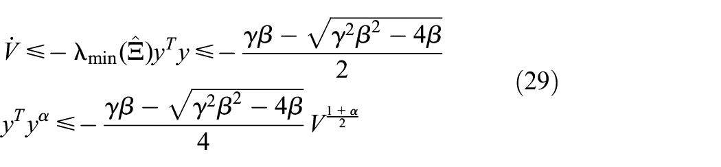
It is easy to find that , that is, Then, we have
According to Lemma 4, we have in finite time, that is
Remark 3: In fact, and Therefore, we take the following formation control
Computation of boundary terms
There remains a significant practical difficulty in computing the boundary terms . We now define a number of quantities relating to Voronoi cells. Let and be the boundary of and , respectively. By we mean a point , and is the outward facing unit normal of . Given an agent i, we define as the index set of robots that share Voronoi boundaries with , . We denote the set of points on the Voronoi boundary shared by agents and as , as shown in Figure 3. Then, is a point on that shared boundary, and is the unit normal of from to . By the definition of the Voronoi cell (3), we know the following facts
where and are matrices. Since points on the boundary of the environment do not change position as a function of , we have . Then, we have
Quantities and constraints associated with the Voronoi boundary shared between neighboring agents.
We will exploit the geometry of the Voronoi cell to derive a parametric formula for the computation of . Define by
where , are the end points of the line segment . Now we can write for . By the definition of the Voronoi cell, any point must satisfy
and
Differentiate (36) implicitly with respect to to find the relation
and
Simplify and substitute using to find the desired formula
where is the identity matrix. Notice (39) is linear in and can be computed readily given the known quantities , and . Then, we can have
where
and
Based on (39) and (41), we have
Remark 4: Similarly, we can obtain the value of . It is easy to find that value of contains . However, can not be exactly obtained in practice. Therefore, we need to consider the error between and . Let , then, we have
Let , then (43) can be rewritten as , where
Then, we have
First, a lemma is introduced as follows.
Lemma 5: Consider the system . Suppose that there exist continuous function , scalars , and such that
Then, the trajectory of system is PFS (Practical Finite-time Stable), and the trajectories of the closed-loop system is bounded in finite time as
where . And the time is bounded as
Because of , then
where , then in terms of Lemma 5, converges a bounded set
in a finite time. And the finite time is where
Coverage tracking algorithm
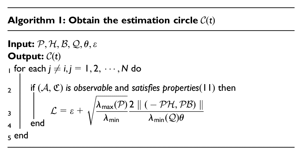
In this section, the coverage tracking algorithmic is given. First, we need to execute Algorithm 1 to obtain the estimation circle . Then, the agents execute Algorithm 2 to construct of cell . Last, the agents begin to execute Algorithm 3 to obtain and make finite time dynamic formation implementation.
Algorithm 1:
Input: Output: 1 for each do 2 if and then 3 4 end 5 end
Algorithm 2: Partitioning – Construction of cell
Input: Output: 1 is obtained; 2 for each do 3 if then 4}; 5 end 6 end
Algorithm 3: Control – Calculation of control laws
Input: Output: 1whiletransmit and receive transmissions from other agentsdo 2, execute Partitioning algorithm; 3for each do 4if, ,,,and are obtained then 5ifthen 6 compute and , and 7ifthen 8 the control law is given as (21) 9end 10end 11end 12end 13end
In order to implement in an algorithmic manner the partitioning scheme and control law, the sensing regions and cells need to be approximated by polygons. In order to calculate the value of the control law, several line integrals have to be calculated numerically as well as one double integral. The line integrals are calculated as sums, each term of which is evaluated on an edge of polygon . The double integral is just the area of the corresponding cell and can thus be calculated simply as the area of the polygonal approximation of that cell. Since cells may consist of multiple disjoint regions or have holes, their polygonal approximations may have multiple contours, internal or external.
Numerical simulations
In order to illustrate the theoretical results, some numerical simulations are presented to validate our coverage algorithms.
The initial position of four agents are , The actuation range of the agent is and the system matrices of the moving target are
The disturbances are given as follows, , . In this example, let
Case 1: The probability density function of the real target appear is the normal distribution probability function.
In order to make the regional integrals easy, we select the circumscribing square of the target region as the new target region. The projection of the initial position and final position of the four agents are shown in Figure 4 (left). It is easy to find that projection of the initial position in the region are grouped, and the projection of the final position in the region are scattered. The projections of the trajectories of the agents on the region of interest can be seen in Figure 4 (left), and the final positions of the agents are marked by asterisks. The change curve of coverage performance index function is shown in Figure 4 (right) and the index function converges to a constant value over time.
The trajectories of four agents on and Value of .
Case 2: The probability density function of the real target appear is uniform.
The projection of the initial position and final position of the four agents are shown in Figure 5 (left). It is easy to find that projection of the initial position in the region are grouped, and the projection of the final position in the region are scattered, which is different from the Case 1. The projections of the trajectories of the agents on the region can be seen in Figure 5 (left), and the final positions of the agents are marked by asterisks. The change curve of coverage performance index function is shown in Figure 5 (right) and the index function converges to a constant value over time. It is easy to find that the convergence rata in Case 1 is greater than the Case 2, which means that the non-uniform probability distribution is beneficial to the coverage of the moving region.
The trajectories of four agents on and value of .
Conclusions and future work
In this paper, we considered a multi-agent tracking problem to cover a moving target in finite time. Since the sensors could not get the exact position and velocity of the moving target, we reconstructed the variables with help of observer design first. Also, based on the observer, we have a circle to denote the region where the target may appear and the probability that the target appear in the circle is denoted by a probability density function. Then a performance index function is given to describe the effectiveness of covering a moving target. Last, a formation-based tracking method was proposed to cover the estimation region of the target in finite time so as to catch it by networked agents.
In the recent work, a general approach that agents are used to cover a moving and fixed size region to guarantee the moving target is covered. However, in the practical problem, the estimation region of the target is time varying. Thus, how to cover the moving and time varying region is a new problem to solve. The future research will focus on this issue.
Footnotes
Declaration of conflicting interests
The author(s) declared no potential conflicts of interest with respect to the research, authorship, and/or publication of this article.
Funding
The author(s) disclosed receipt of the following financial support for the research, authorship, and/or publication of this article: This work is partially supported by the National Key Research and Development Project (Grant No. 2018YFE0208700) and Special Research Project of Chinese Civil Aircraft (No. MJ-2020-S-03).
ORCID iD
Longbiao Ma
References
1.
ArslanOKoditschekDE (2016) Voronoi-based coverage control of heterogeneous disk-shaped robots. In: 2016 IEEE International Conference on Robotics and Automation, Stockholm, Sweden, 16–21 May 2016, pp. 1–8. Stockholm: Institute of Electrical and Electronic Engineers.
2.
BikramadityaDBidyadharSBibhutiBP (2016) Co-operative control coordination of a team of underwater vehicles with communication constraints. Transactions of the Institute of Measurement and Control38(4): 463–481.
GuptaHPRaoSVTamarapalliV (2015) Analysis of stochastic k-coverage and connectivity in sensor networks with boundary deployment. IEEE Transactions on Intelligent Transportation Systems16(4): 1–11.
8.
GusrialdiAHircheSAsikinD (2009) Voronoi-based coverage control with anisotropic sensors and experimental case study. Intelligent Service Robotics2(4): 195–204.
9.
HusseinIIStipanovicDM (2007) Effective coverage control for mobile sensor networks with guaranteed collision avoidance. IEEE Transactions on Control Systems Technology15(4): 642–657.
10.
LeonardNEOlshevskyA (2013) Nonuniform coverage control on the line. IEEE Transactions on Automatic Control58(11): 2743–2755.
11.
LiuCWuKXiaoY (2006) Random coverage with guaranteed connectivity: Joint scheduling for wireless sensor networks. IEEE Transactions on Parallel & Distributed Systems17(6): 562–575.
12.
LiuRYangFZhangH (2018) Path planning for UAV based on improved chaotic ant colony algorithm (CACA). Command Information System and Technology9(6): 41–48.
13.
LuoQ (2012) Barrier coverage control based on data fusion for wireless sensor network. Journal of Electronics & Information Technology34(4): 825–831.
14.
LuoQLiRKShaoWW (2018) Design of intelligent path planning for tactical enviroment. Command Information System and Technology9(6): 49–54.
15.
MiahSBaoNBourqueA (2015) Nonuniform coverage control with stochastic intermittent communication. IEEE Transactions on Automatic Control60(7): 1981–1986.
16.
NasimovMMatveevA (2015) Suboptimal decentralized blanket coverage control of mobile autonomous sensor networks. In: 2014 6th International Congress on Ultra Modern Telecommunications and Control Systems and Workshops (ICUMT), St. Petersburg, Russia, 6–8 October 2014, pp. 366-371. St. Petersburg: Institute of Electrical and Electronic Engineers.
17.
SavkinAChengTXiZ (2015) Decentralized Coverage Control Problems for Mobile Robotic Sensor and Actuator Networks. John Wiley & Sons.
18.
SunZLiLWangH (2015) A novel energy efficient multi-target coverage control protocol with event driven mechanism of wireless sensor network. In: 2015 International Conference on Identification, Information, and Knowledge in the Internet of Things, Beijing, China, 22–23 October 2015, pp. 201-205. Beijing: Institute of Electrical and Electronic Engineers.
19.
WangXLHongYG (2008) Finite-time consensus for multi-agent networks with second-order agent dynamics. IFAC Proceedings Volumes41(2): 15185–15190.
20.
WangXLWuJ (2012) Coverage tracking control for multiple cooperative agents. International Journal of Control85(6): 660–670.
21.
WangXLHongYGJiangZP (2009) Coverage tracking of a moving target by a group of mobile agents. In: 2009 7th Asian Control Conference, Hong Kong, China, 27–29 August 2009, pp. 332–337. Hong Kong: Institute of Electrical and Electronic Engineers.
22.
WangYHusseinII (2007) Cooperative vision-based multi-vehicle dynamic coverage control for underwater applications. In: 2007 IEEE International Conference on Control Applications, Singapore, Singapore, 1–3 October 2007, pp. 82–87. Singapore: Institute of Electrical and Electronic Engineers.
23.
ZuoLChenWCuiR (2014) Coverage control of multiple autonomous underwater vehicle with disturbance by ocean currents considered. Journal of Northwestern Polytechnical University32(5): 769–774.