Fixed-time tracking control for two-link rigid manipulator based on disturbance observer

Abstract

This paper studies the fixed-time disturbance estimate and tracking control for two-link manipulators subjected to external disturbance. A fixed-time extended-state disturbance observer (FxTESDO) is proposed by improving the extended state observer. Also, a fixed-time inverse dynamics tracking control (FxTIDTC) scheme based on the FxTESDO is given for two-link manipulators. The fixed-time convergence of the FxTESDO and FxTIDTC is proved by the Lyapunov stability theory and with the aid of the bi-limit homogeneous technique. Numerical simulations are employed to illustrate the effectiveness of the proposed FxTIDTC.

Keywords

Trajectory tracking inverse dynamics control disturbance observer bi-limit homogeneous fixed-time stability

Introduction

With the continuous development and maturity of robot technology, robot manipulators are further applied to industry, agriculture, medical treatment, and space exploration (see, for example, Cao et al. (2019), Chen et al. (2019), Huang et al. (2016), Kawamura et al. (2016), Li et al. (2016) and Trujillo et al. (2019)), and so forth. Manipulators are multi-input and multi-output (MIMO) systems with strong nonlinearity and coupling. In addition, external disturbances and modelling uncertainty are also the difficulties to obtain the high-quality trajectory tracking control for manipulators. To overcome these adverse factors, various methods have been proposed by control theorists and engineers, such as adaptive control, intelligent control, neural network control and sliding mode control (see, for example, Baek et al. (2016), Chen et al. (2020a), Chen et al. (2020b), Ertugrul and Kaynak (2000), Ferrara and Incremona (2015), Gueaieb et al. (2007), He et al. (2015), Kim (2004), Lee et al. (2009), Li et al. (2013), Patiño et al. (2002) and Sun and Wang (2005)). However, fast trajectory tracking is also required in many applications in addition to system stability. Therefore, developing control methods with fast convergence to velocity is particularly essential. In such a context, finite-time and fixed-time control are proposed successively. However, there are few researches on the fixed-time tracking control for manipulators subjected to external disturbances. Thus, improved design for fixed-time disturbance estimation and fixed-time trajectory tracking of two-link manipulators subjected to external disturbance will be considered in this paper.

Speaking of fixed-time control (FxTC), we have to pay attention to the finite-time control (FTC), which has been widely concerned. The system remains stable within a finite-time time T under the FTC. Terminal sliding mode control (TSMC) as a main method of FTC was first developed by Venkataraman and Gulati (1993), in which the concept of terminal sliding surfaces was proposed and applied to the finite-time control of a nonlinear system. Driven by the advantages of TSMC such as the finite-time stability, various improved methods base on TSMC have been applied to manipulator controlling, such as Chiu (2012), Feng et al. (2002), Wang et al. (2009) and Yang and Yang (2011). Another important method of FTC is the homogeneity technique. For example, the result of Bhat and Bernstein (1997) indicated that if a homogeneous system with a negative degree is asymptotically stable, it is finite-time stable. Inspired by this result, FTC for a manipulator system was proposed in Hong et al. (2002) through both dynamic output feedback and state feedback control. Then, its main results were employed by Galicki (2015) to propose a class of FTC for a rigid manipulator with uncertain dynamic and globally unbounded disturbances. This scheme was later refined by Galicki (2016). However, the so-called settling-time T of FTC is dependent on the initial condition $x_{0}$ of the system, which leads to the possibility that T will increase with the increase of $x_{0}$ . Therefore, people have developed FxTC as an extension of FTC (see, for example, Ni et al. (2017), Polyakov (2012), Zhang and Wu (2017), Zuo (2015a) and Zuo (2015b)). The system can be stable within a fixed-time time T under the FxTC, where $T \leq T_{\max}$ and $T_{\max}$ is independent of the initial conditions. Many schemes of FxTC were realized by introducing higher-order power terms based on the FTC-related schemes, and the fixed-time convergence of the FxTC is verified using the bi-limit homogeneous technique. For instance, FxTC for double-integrator systems was designed by Tian et al. (2017) using the bi-limit homogeneous technique of Andrieu et al. (2008). Higher-order sliding mode observer was employed by Basin et al. (2017) to study both finite and fixed settling time of differentiators, where the fixed-time observer was to add higher-order power terms to the finite-time observer. Fixed-time inverse dynamics control (FxTIDC) was designed for a robot manipulator without disturbances by Su and Zheng (2019) on the basis of modifying the FTC scheme of Su (2009). Although simulation results in these works of literature have indicated that FxTC has good robustness to external disturbances, and the FxTC with high anti-disturbance ability needs to be further studied, which is also the motivation of this paper.

Disturbances observer (DO) is usually employed in engineering practice, to suppress external disturbances and system uncertainty (see, for example, Chen and Ge (2013), Han et al. (2019), Li et al. (2018), Sun et al. (2019), Yang et al. (2018), Yang et al. (2013), Yang et al. (2008) and Zheng and Chen (2018)). For instance, an enhanced nonlinear DO was derived by Chen et al. (2000) to estimate the constant disturbance of robotic manipulators. A nonlinear DO for disturbances generated by a general liner system was proposed by Chen (2004), with its global exponential stability established. To deal with ramp disturbance, a high-order DO was proposed by Kim et al. (2010), to cope with general order disturbances. Recently, the problem of fixed-time estimation of disturbances has attracted wide attention. In Ni et al. (2018), a fixed-time disturbance observer (FxTDO) with adjustment switch was designed for Brunovsky systems to estimate the external disturbance and its i th derivatives. Wu et al. (2017) proposed a FxTDO for second-order uncertain systems based on the results of Andrieu et al. (2008). However, FxTDO for the two-link manipulator system still needs to be further developed.

Therefore, fixed-time inverse dynamics tracking control (FxTIDTC) is proposed in this paper for two-link manipulators subjected to external disturbances. Under the assumption that the external disturbances are bounded, fixed-time stability of the tracking error system is proved with Lyapunov’s direct method and the bi-limit homogeneous technique. Moreover, to achieve FxTC with small gains, a fixed-time extended-state disturbance observer (FxTESDO) is also proposed by improving the extended state observer (ESO). Theoretical results confirm that the proposed FxTIDTC based on the FxTESDO can realize fixed-time tracking. And, the simulation results indicate that it has desired control performance. The main contribution of this paper is not only to provide a theoretical basis for the robustness of FxTC against external disturbances, but also to offer an improved design for faster disturbance estimation and high-accuracy trajectory tracking of manipulators.

The rest of the sections are arranged as follows. The model of the two-link manipulator to be studied, as well as some definitions and lemmas to be used in the subsequent analysis are given in Section 2. In Section 3, inspired by Wu et al. (2017), a bi-limit-weighted homogeneous FxTESDO is proposed in which the coefficients are not all constants, and the fixed-time convergence of the FxTESDO is proved. FxTIDTC based on the FxTESDO is given for the two-link manipulator in Section 4. In Section 5, numerical simulation is employed to illustrate the effectiveness of the proposed FxTIDTC. In Section 6, some conclusions are drawn.

Notations:

$R_{+}$ denotes the set $[0, + \infty)$ .

$\forall x = [x_{1}, x_{2}, \dots, x_{n}]^{T} \in R^{n}$ , let $∥ x ∥ = \sqrt{x^{T} x}$ , and $| x | = [| x_{1} |, | x_{2} |, \dots, | x_{n} |]^{T}$ .

$\forall x \in R$ and $ν \in R_{+} \ {0}$ , denote $si g^{ν} (x) = | x |^{ν} sign (x)$ , where

sign (x) = {\begin{matrix} 1, x > 0, \\ 0, x = 0, \\ - 1, x < 0 . \end{matrix}

According to this definition, the following equation holds

\frac{dsi g^{ν} (x)}{dx} = ν | x |^{ν - 1} .

$\forall x \in R^{n}$ and $ν \in R_{+} \ {0}$ , the vector field function $x \to si g^{ν} (x)$ is defined as

$si g^{ν} (x) = {[si g^{ν} (x_{1}), si g^{ν} (x_{2}), \dots, si g^{ν} (x_{n})]}^{T} .$

For any selected vector $r = {r_{i}}_{i = 1}^{n}$ , where $r_{i} \in R_{+} \ {0}$ , define the matrix

Λ_{r} (λ) = diag {λ^{r_{i}}}_{i = 1}^{n}, \forall λ \in R_{+} \ {0} .

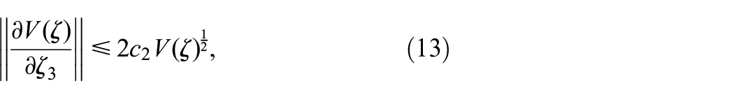
Let $I \in R^{n \times n}$ denote the identity matrix, and $O \in R^{n \times n}$ denotes the null matrix.

For the matrix $A = [a_{ij}]_{n \times n}$ , denote $| A | = \det (A)$ and the matrix norm is given by

∥ A ∥ = max_{x \neq 0} \frac{‖ A x ‖}{‖ x ‖} .

Problem statement and preliminaries

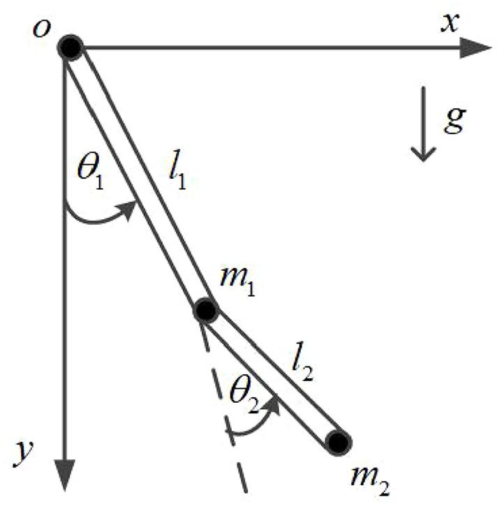
The two-link manipulator (Zheng and Chen, 2018) with the structure shown in Figure 1 is considered in this paper.

Figure 1.

Structure of the two-link manipulator.

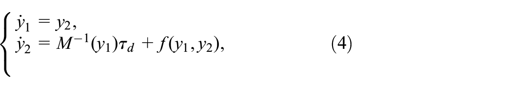
According to the analysis in Zheng and Chen (2018), the dynamic model of the two-link manipulator is

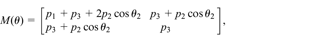
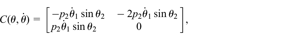
M (θ) \overset{\cdot\cdot}{θ} + C (θ, \overset{\cdot}{θ}) \overset{\cdot}{θ} + G (θ) = τ + τ_{d},

(1)

where $θ = {[θ_{1}, θ_{2}]}^{T}$ denotes the joint positions, $\overset{\cdot}{θ}$ and $\overset{\cdot\cdot}{θ}$ represent the velocity and acceleration, respectively, $M (θ) \in R^{2 \times 2}$ is the symmetric inertial matrix, $C (θ, \overset{\cdot}{θ}) \in R^{2}$ refers to the centrifugal-Coriolis matrix, and $G (θ) \in R^{2}$ denotes the influence of gravity. The corresponding items are represented as follows (Zheng and Chen, 2018)

M (θ) = [\begin{matrix} p_{1} + p_{3} + 2 p_{2} \cos θ_{2} p_{3} + p_{2} \cos θ_{2} \\ p_{3} + p_{2} \cos θ_{2} p_{3} \end{matrix}],

C (θ, \overset{\cdot}{θ}) = [\begin{matrix} - p_{2} {\overset{\cdot}{θ}}_{1} \sin θ_{2} - 2 p_{2} {\overset{\cdot}{θ}}_{1} \sin θ_{2} \\ p_{2} {\overset{\cdot}{θ}}_{1} \sin θ_{2} 0 \end{matrix}],

G (θ) = [\begin{matrix} p_{4} \sin θ_{2} + p_{5} \sin (θ_{1} + θ_{2}) \\ p_{5} \sin (θ_{1} + θ_{2}) \end{matrix}],

in which

p_{1} = (m_{1} + m_{2}) l_{1}^{2}, p_{2} = m_{2} l_{1} l_{2}, p_{3} = m_{2} l_{2}^{2},

p_{4} = (m_{1} + m_{2}) g l_{1}, p_{5} = m_{2} g l_{2},

where $m_{1}$ , $m_{2}$ are the masses, $l_{1}$ , $l_{2}$ are the lengths of the two links, $τ = {[τ_{1}, τ_{2}]}^{T}$ denotes the input torque, and $τ_{d} = [τ_{d 1}, τ_{d 2}]^{T}$ is unknown external time-varying disturbance.

It is well-known that $M (θ)$ is a positive definite and bounded matrix (Spong et al., 2004: 218). Therefore, $M^{- 1} (θ)$ is a positive definite matrix which has

λ_{m} \leq ∥ M^{- 1} (θ) ∥ \leq λ_{M},

(2)

where $λ_{m}$ ( $λ_{M} < \infty$ ) denotes the strictly positive minimum (maximum) eigenvalue of $M^{- 1} (θ)$ for all joint position $θ$ .

Assumption 1: Supposing that $τ_{d}$ in system (1) is differentiable and its derivative is bounded, that is, there is a positive real number $u_{1}$ which makes $∥ {\overset{\cdot}{τ}}_{d} ∥ \leq u_{1}$ .

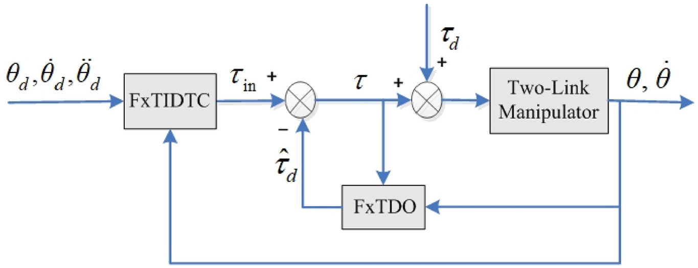
Our goal is to design a closed-loop controlled system as shown in Figure 2, where the designed FxTESDO can realize fixed-time estimation of $τ_{d}$ , and FxTIDTC can ensure fixed-time trajectory tracking for the expected tracking signals $θ_{d}$ and ${\overset{\cdot}{θ}}_{d}$ . To achieve this goal, the following preliminaries are essential.

Figure 2.

Diagram of the controlled manipulator system.

Assume that the origin of the following system is equilibrium

\overset{\cdot}{y} (t) = f (y (t)), y (0) = y_{0},

(3)

where $y \in R^{n}$ , and $f : R^{n} \to R^{n}$ is a nonlinear vector field function.

Definition 1: (Bhat and Bernstein, 2000; Polyakov, 2012) The system (3) is said to be (globally) finite-time stable, if it is (globally) Lyapunov stable and there exists a function $T : R^{n} \to (0, + \infty)$ , which is called the settling-time function. For every initial condition $y_{0} \in R^{n}$ , all solutions of system (3) satisfy

y (t, y_{0}) = 0, \forall t \geq T .

Moreover, if there is a positive constant $T_{\max}$ which is independent of $y_{0}$ , such that $T \leq T_{\max}$ , then, the origin is said to be (globally) fixed-time stable.

Definition 2: (Polyakov and Fridman, 2014) If $y (t, y_{0}) = 0$ is not satisfied in Definition 2.1, but for all $t \geq T$ , we have $y (t, y_{0}) \in O,$ where $O \subset R^{n}$ is an open neighbourhood of the the origin, the system (3) is called finite-time (resp. fixed-time if $T \leq T_{\max}$ ) convergent to $O$ .

Definition 3: (Bernuau et al., 2014) A function $v : R^{n} \to R$ (resp. $f : R^{n} \to R^{n}$ ) is said to be homogeneous of degree $d \in R$ with respect to a generalized weight $r$ , if $\forall λ > 0$ and $y \in R^{n}$ ,

v (Λ_{r} (λ) y) = λ^{d} v (y)

(resp . λ^{- d} Λ_{r}^{- 1} (λ) f (Λ_{r} (λ) y) = f (y)) .

Definition 4: (Andrieu et al., 2008) If for any compact subset $C \subset R^{n} \ {0}$ and constant $δ > 0$ , there exists a positive real constant $λ_{p} > 0$ ( $p = 0 or \infty$ ), such that $\forall λ \leq λ_{0} or \forall λ \geq λ_{\infty},$ the function $v : R^{n} \to R$ satisfies

max_{y \in C} | λ^{- d_{p}} v (Λ_{r_{p}} (λ) y) - v_{p} (y) | \leq δ,

(resp . \forall λ \leq λ_{0} or \forall λ \geq λ_{\infty}, f : R^{n} \to R^{n} satisfies

max_{y \in C} ∥ λ^{- d_{p}} Λ_{r_{p}}^{- 1} (λ) f (Λ_{r_{p}} (λ) y) - f_{p} (y) ∥ \leq δ),

the function v (resp. vector field f) is said to be homogeneous in the p-limit with a associated triple $(r_{p}, d_{p}, v_{p})$ (resp. $(r_{p}, d_{p}, f_{p})$ ). The approximating function $v_{p} : R^{n} \to R$ (resp. $f_{p} : R^{n} \to R^{n}$ ) is homogeneous of degree $d_{p}$ with respect to the generalized weight $r_{p}$ . A function $v : R^{n} \to R$ (resp. $f : R^{n} \to R^{n}$ ) is said to be homogeneous in the bi-limit, if it is both homogeneous in the 0-limit and in the $\infty$ -limit.

For the convenience of the following analysis, $H^{b}$ is denoted as the set of functions that are homogeneous in the bi-limit.

Our control approach will be developed based on the following lemmas.

Lemma 1: (Corollary 2.15 in Andrieu et al. (2008)) Consider two functions $ϕ : R^{n} \to R$ and $φ : R^{n} \to R_{+}$ . Assume that $ϕ \in H^{b}$ with associated triples $(r_{p}, d_{ϕ_{p}}, ϕ_{p})$ ( $p = 0$ or $\infty$ ), and $φ \in H^{b}$ with associated triples $(r_{p}, d_{φ_{p}}, φ_{p})$ ( $p = 0$ or $\infty$ ). Also, the functions $φ, φ_{0}, φ_{\infty}$ are positive definite. Then, if $d_{ϕ_{0}} \geq d_{φ_{0}}$ and $d_{ϕ_{\infty}} \leq d_{φ_{\infty}}$ , we have

ϕ (y) < c φ (y), \forall y \in R^{n},

where c is a positive real constant.

Lemma 2: (Theorem 2.20 in Andrieu et al. (2008)) Consider a vector field $f : R^{n} \to R^{n}$ . Assume that $f \in H^{b}$ with associated triples $(r_{p}, d_{p}, f_{p})$ ( $p = 0$ or $\infty$ ), $d_{V_{0}}$ and $d_{V_{\infty}}$ are real constants such that $d_{V_{0}} > max_{1 \leq i \leq n} r_{0, i}$ and $d_{V_{\infty}} > max_{1 \leq i \leq n} r_{\infty, i}$ . Then, if the following systems are globally asymptotically stable

\overset{\cdot}{y} = f (y), \overset{\cdot}{y} = f_{0} (y), \overset{\cdot}{y} = f_{\infty} (y),

we have a positive definite and proper function $V : R^{n} \to R_{+}$ that satisfies

(1) For each $i \in {1, 2, \dots, n}$ , $\frac{\partial V}{\partial y_{i}} \in H^{b}$ with associated triples $(r_{p}, d_{V_{p}} - r_{p, i}, \frac{\partial V_{p}}{\partial y_{i}})$ ( $p = 0$ or $\infty$ ).

(2) The following functions are negative definite

y \mapsto \frac{\partial V}{\partial y} f (y), y \mapsto \frac{\partial V_{0}}{\partial y} f_{0} (y), y \mapsto \frac{\partial V_{\infty}}{\partial y} f_{\infty} (y) .

Lemma 3: (Corollary 2.24 in Andrieu et al. (2008)) Under the assumptions in Lemma 2.2, and supposing $d_{\infty} > 0 > d_{0}$ , all solutions of the system $\overset{\cdot}{y} = f (y)$ converge to the origin within a time t which has

t \leq c (\frac{d_{V_{\infty}}}{| d_{\infty} |} + \frac{d_{V_{0}}}{| d_{0} |}),

where c is a positive real constant.

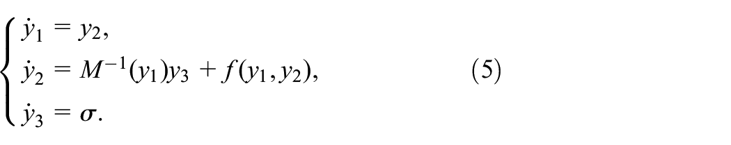
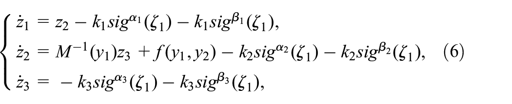
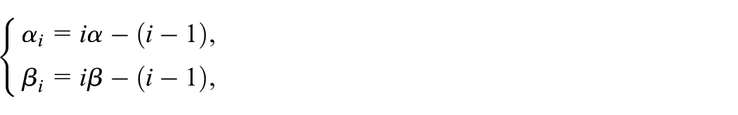
Design of fixed-time disturbance observer

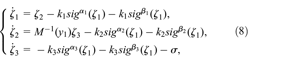
A FxTESDO for $τ_{d}$ in system (1) will be proposed in this section, by improving the ESO. And, the fixed-time estimation of the FxESTDO will be proved, by using the Lyapunov stability theory and the bi-limit homogeneous technique.

Defining $y_{1} = θ$ , $y_{2} = \overset{\cdot}{θ}$ and

f (y_{1}, y_{2}) = M^{- 1} (y_{1}) [- C (y_{1}, y_{2}) y_{1} - G (y_{1}) + τ],

we can rewrite system (1) as

{\begin{matrix} {\overset{\cdot}{y}}_{1} = y_{2}, \\ {\overset{\cdot}{y}}_{2} = M^{- 1} (y_{1}) τ_{d} + f (y_{1}, y_{2}), \end{matrix}

(4)

Following the design idea of ESO (see Han, 2009), let us treat $τ_{d}$ as an additional state variable $y_{3}$ . Define $σ (t) = {\overset{\cdot}{τ}}_{d}$ , and then, system (4) is now described as

{\begin{matrix} {\overset{\cdot}{y}}_{1} = y_{2}, \\ {\overset{\cdot}{y}}_{2} = M^{- 1} (y_{1}) y_{3} + f (y_{1}, y_{2}), \\ {\overset{\cdot}{y}}_{3} = σ . \end{matrix}

(5)

Now, inspired by the FxTDO in Wu et al. (2017), a FxTESDO is designed in the form of

{\begin{matrix} {\overset{\cdot}{z}}_{1} = z_{2} - k_{1} si g^{α_{1}} (ζ_{1}) - k_{1} si g^{β_{1}} (ζ_{1}), \\ {\overset{\cdot}{z}}_{2} = M^{- 1} (y_{1}) z_{3} + f (y_{1}, y_{2}) - k_{2} si g^{α_{2}} (ζ_{1}) - k_{2} si g^{β_{2}} (ζ_{1}), \\ {\overset{\cdot}{z}}_{3} = - k_{3} si g^{α_{3}} (ζ_{1}) - k_{3} si g^{β_{3}} (ζ_{1}), \end{matrix}

(6)

in which $z_{1}$ , $z_{2}$ , $z_{3}$ are estimations for $y_{1}$ , $y_{2}$ , $y_{3}$ , respectively, $ζ_{i} = z_{i} - y_{i}$ $(i = 1, 2, 3)$ are estimation errors, and the parameters can be designed to satisfy the following conditions:

C1: For $i = 1, 2, 3,$ the exponents $α_{i}$ and $β_{i}$ are designed as those by Basin et al. (2017)

{\begin{matrix} α_{i} = i α - (i - 1), \\ β_{i} = i β - (i - 1), \end{matrix}

where $α \in (1 - 1 / 3, 1)$ , $β \in (1, 1 + 1 / 3)$ .

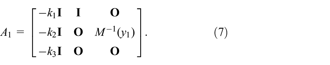
C2: For $i = 1, 2, 3,$ the coefficients $k_{i}$ are all positive real constants that satisfy $k_{1} k_{2} > 2 k_{3} λ_{M}$ , so the matrix $A_{1}$ in the following is Hurwitz (see Appendix A)

A_{1} = [\begin{matrix} - k_{1} I & I & O \\ - k_{2} I & O & M^{- 1} (y_{1}) \\ - k_{3} I & O & O \end{matrix}] .

(7)

All the above analysis of the DO in (6) can be summarized as a theorem, as shown below.

Theorem 1: If Assumption 1 holds and the design of parameters $α_{i}$ , $β_{i}$ and $k_{i}$ satisfies the conditions (C1) and (C2), the DO in (6) for the system (1) is a FxTDO. That is to say, for any initial conditions of the systems (5) and (6), supposing ${\overset{\cdot}{τ}}_{d} = 0$ , $ζ_{i}$ uniformly converges to the origin at a time $t_{o}$ upper bounded by $T_{\max, 1}$ , which is independent of the initial conditions. Supposing ${\overset{\cdot}{τ}}_{d} \neq 0$ , $ζ_{i}$ uniformly converges to $O$ at a time $t_{o} \leq T_{\max, 1}$ , where $O$ is a neighborhood of the origin.

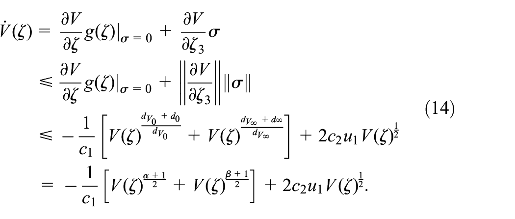
Proof: Considering the systems (5) and (6), a direct computation shows that $ζ = [ζ_{1}, ζ_{2}, ζ_{3}]^{T}$ satisfies

{\begin{matrix} {\overset{\cdot}{ζ}}_{1} = ζ_{2} - k_{1} si g^{α_{1}} (ζ_{1}) - k_{1} si g^{β_{1}} (ζ_{1}), \\ {\overset{\cdot}{ζ}}_{2} = M^{- 1} (y_{1}) ζ_{3} - k_{2} si g^{α_{2}} (ζ_{1}) - k_{2} si g^{β_{2}} (ζ_{1}), \\ {\overset{\cdot}{ζ}}_{3} = - k_{3} si g^{α_{3}} (ζ_{1}) - k_{3} si g^{β_{3}} (ζ_{1}) - σ, \end{matrix}

(8)

which can be written as $\overset{\cdot}{ζ} = g (ζ)$ .

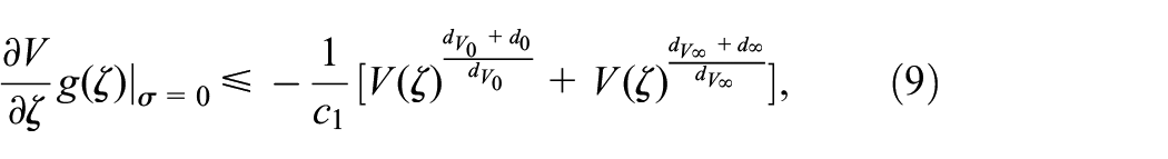
Next, we will complete the proof in two steps. Supposing $σ = 0$ , the fixed-time stability of $\overset{\cdot}{ζ} = g (ζ) |_{σ = 0}$ is analyzed in Step 1. While in Step 2, we obtain the region of steady-state errors when $σ \neq 0$ .

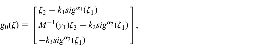
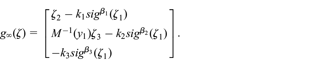
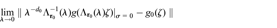
Step 1: Supposing $σ = 0$ , let us define two approximation vector filed functions of $g (ζ) |_{σ = 0}$ as

g_{0} (ζ) = [\begin{matrix} ζ_{2} - k_{1} si g^{α_{1}} (ζ_{1}) \\ M^{- 1} (y_{1}) ζ_{3} - k_{2} si g^{α_{2}} (ζ_{1}) \\ - k_{3} si g^{α_{3}} (ζ_{1}) \end{matrix}],

g_{\infty} (ζ) = [\begin{matrix} ζ_{2} - k_{1} si g^{β_{1}} (ζ_{1}) \\ M^{- 1} (y_{1}) ζ_{3} - k_{2} si g^{β_{2}} (ζ_{1}) \\ - k_{3} si g^{β_{3}} (ζ_{1}) \end{matrix}] .

Firstly, according to Definition 3, $g_{0} (ζ)$ and $g_{\infty} (ζ)$ are homogeneous of degree $d_{0} = α - 1$ and $d_{\infty} = β - 1$ with respect to $r_{0} = {1, α_{1}, α_{2}}$ and $r_{\infty} = {1, β_{1}, β_{2}}$ , respectively. Then, it is easy to verify that $g (ζ) |_{σ = 0} \in H^{b}$ with associated triples $(r_{p}, d_{p}, g_{p})$ ( $p = 0$ or $\infty$ ), by simply noting the following facts

lim_{λ \to 0} ∥ λ^{- d_{0}} Λ_{r_{0}}^{- 1} (λ) g (Λ_{r_{0}} (λ) ζ) |_{σ = 0} - g_{0} (ζ) ∥

= lim_{λ \to 0} ∥ [Λ_{1}, Λ_{2}, Λ_{3}]^{T} ∥ = 0,

lim_{λ \to + \infty} ∥ λ^{- d_{\infty}} Λ_{r_{\infty}}^{- 1} (λ) g (Λ_{r_{\infty}} (λ) ζ) |_{σ = 0} - g_{\infty} (ζ) ∥

= lim_{λ \to + \infty} ∥ [Θ_{1}, Θ_{2}, Θ_{3}]^{T} ∥ = 0,

in which for $i = 1, 2, 3,$

Λ_{i} = - λ^{i (β - α)} k_{i} si g^{β_{i}} (ζ_{1}),

and

Θ_{i} = - λ^{i (α - β)} k_{i} si g^{α_{i}} (ζ_{1}) .

Secondly, due to the fact that the coefficient matrix $A_{1}$ defined in (7) is Hurwitz, the origins of systems $\overset{\cdot}{ζ} = g_{0} (ζ)$ and $\overset{\cdot}{ζ} = g_{\infty} (ζ)$ are globally asymptotically equilibrium (see Ni et al., 2018). Thus, the origin of system $\overset{\cdot}{ζ} = g (ζ) |_{σ = 0}$ is globally asymptotically equilibrium, according to the Propositions 2.16 and 2.18 in Andrieu et al. (2008).

Therefore, if we choose two real numbers

d_{V_{0}} = 2 > \max {1, α_{1}, α_{2}},

and

d_{V_{\infty}} = 2 > \max {1, β_{1}, β_{2}},

according to Lemma 2 in this paper and Theorem 2 in Rosier (1992), we have a Lyapunov function $V (ζ)$ of system $\overset{\cdot}{ζ} = g (ζ) |_{σ = 0}$ with the following properties:

P1: $V (ζ) \in H^{b}$ with associated triples $(r_{p}, d_{V_{p}}, V_{p} (ζ))$ ( $p = 0 or \infty$ ), where the Lyapunov function $V_{p} (ζ)$ of system $\overset{\cdot}{ζ} = g_{p} (ζ)$ is homogeneous of degree $d_{V_{p}}$ with respect to $r_{p}$ .

P2: The following functions are negative definite

$ζ \mapsto \frac{\partial V}{\partial ζ} g (ζ) |_{σ = 0}, ζ \mapsto \frac{\partial V_{0}}{\partial ζ} g_{0} (ζ), ζ \mapsto \frac{\partial V_{\infty}}{\partial ζ} g_{\infty} (ζ) .$

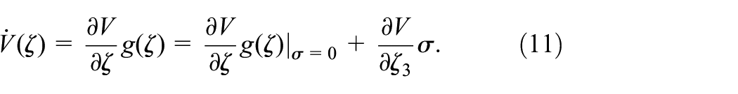
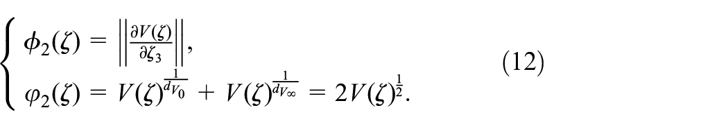
Also, $\frac{\partial V}{\partial ζ_{i}} \in H^{b}$ with associated triples $(r_{p}, d_{V_{p}} - r_{p, i}, \frac{\partial V_{p}}{\partial ζ_{i}})$ ( $p = 0 or \infty$ ).

Thirdly, letting $\overset{\cdot}{V} (ζ)$ denote the derivative of $V (ζ)$ along $\overset{\cdot}{ζ} = g (ζ) |_{σ = 0}$ . According to the properties of homogeneity (see Basin et al., 2017) and the above properties (P1–P2), we obtain $\overset{\cdot}{V} (ζ) \in H^{b}$ with associated triples $(r_{p}, d_{V_{p}} + d_{p}, {\overset{\cdot}{V}}_{p} (ζ))$ ( $p = 0$ or $\infty$ ), and $\overset{\cdot}{V} (ζ)$ is negative definite. Now, define two functions $ϕ_{1} (ζ)$ and $φ_{1} (ζ)$ as

{\begin{matrix} ϕ_{1} (ζ) = V {(ζ)}^{\frac{d_{V_{0}} + d_{0}}{d_{V_{0}}}} + V {(ζ)}^{\frac{d_{V_{\infty}} + d_{\infty}}{d_{V_{\infty}}}}, \\ φ_{1} (ζ) = - \overset{\cdot}{V} (ζ) = - \frac{\partial V}{\partial ζ} g (ζ {) |}_{σ = 0} . \end{matrix}

Notice that $d_{V_{0}} d_{\infty} > d_{V_{\infty}} d_{0}$ , which enable us to verify that $ϕ_{1} (ζ) \in H^{b}$ with associated triples $(r_{p}, d_{V_{p}} + d_{p}, V_{p} (ζ)^{\frac{d_{V_{p}} + d_{p}}{d_{V_{p}}}})$ ( $p = 0$ or $\infty$ ). Denoting $φ_{1, p} (ζ) = - \frac{\partial V_{p}}{\partial ζ} g (ζ) |_{σ = 0}$ ( $p = 0$ or $\infty$ ), it is easy to verify $φ_{1} (ζ) \in H^{b}$ with associated triples $(r_{p}, d_{V_{p}} + d_{p}, φ_{1, p} (ζ))$ ( $p = 0$ or $\infty$ ). Since $φ_{1} (ζ)$ , $φ_{1, 0} (ζ)$ and $φ_{1, \infty} (ζ)$ are positive definite, according to Lemma 1, we have

ϕ_{1} (ζ) \leq c_{1} φ_{1} (ζ),

that is

\frac{\partial V}{\partial ζ} g (ζ) |_{σ = 0} \leq - \frac{1}{c_{1}} [V (ζ)^{\frac{d_{V_{0}} + d_{0}}{d_{V_{0}}}} + V (ζ)^{\frac{d_{V_{\infty}} + d_{\infty}}{d_{V_{\infty}}}}],

(9)

in which $c_{1}$ is a positive real constant.

Finally, through the above work, vector fields $\overset{\cdot}{ζ} = g (ζ) |_{σ = 0}$ , $\overset{\cdot}{ζ} = g_{0} (ζ)$ and $\overset{\cdot}{ζ} = g_{\infty} (ζ)$ satisfying the hypotheses of Lemma 2 are established, and the homogeneity degrees of approximation functions satisfy $d_{\infty} > 0 > d_{0}$ . Therefore, according to Lemma 3 and Appendix H in Andrieu et al. (2008), all solutions of system $\overset{\cdot}{ζ} = g (ζ) |_{σ = 0}$ converge to the origin within a time $t_{o}$ which has

t_{o} \leq c_{1} (\frac{d_{V_{\infty}}}{d_{\infty}} + \frac{d_{V_{0}}}{| d_{0} |}) = 2 c_{1} (\frac{1}{β - 1} + \frac{1}{1 - α}) : = T_{\max, 1},

(10)

in which $T_{\max, 1}$ is independent of the initial condition.

Step 2: Supposing $σ \neq 0$ , we obtain the full-time derivative of $V (ζ)$ along trajectories of $\overset{\cdot}{ζ} = g (ζ)$ is

\overset{\cdot}{V} (ζ) = \frac{\partial V}{\partial ζ} g (ζ) = \frac{\partial V}{\partial ζ} g (ζ) |_{σ = 0} + \frac{\partial V}{\partial ζ_{3}} σ .

(11)

Consider two functions $ϕ_{2} (ζ)$ and $φ_{2} (ζ)$ defined as

{\begin{matrix} ϕ_{2} (ζ) = ‖ \frac{\partial V (ζ)}{\partial ζ_{3}} ‖, \\ φ_{2} (ζ) = V {(ζ)}^{\frac{1}{d_{V_{0}}}} + V {(ζ)}^{\frac{1}{d_{V_{\infty}}}} = 2 V {(ζ)}^{\frac{1}{2}} . \end{matrix}

(12)

By the property (P2) in Step 1, we have $ϕ_{2} (ζ) \in H^{b}$ with associated triples $(r_{p}, d_{V_{p}} - r_{p, 3}, ‖ \frac{\partial V_{p} (ζ)}{\partial ζ_{3}} ‖)$ ( $p = 0$ or $\infty$ ), and $φ_{2} (ζ) \in H^{b}$ with associated triples $(r_{p}, 1, V_{p} (ζ)^{\frac{1}{2}})$ ( $p = 0$ or $\infty$ ).

Be aware that

d_{ϕ_{2, 0}} = d_{V_{0}} - r_{0, 3} = 2 - (2 α - 1) > 1 = d_{φ_{2, 0}},

d_{ϕ_{2, \infty}} = d_{V_{\infty}} - r_{\infty, 3} = 2 - (2 β - 1) < 1 = d_{φ_{2, \infty}} .

Moreover, the functions $φ_{2} (ζ)$ , $V_{0} (ζ)^{\frac{1}{2}}$ and $V_{\infty} (ζ)^{\frac{1}{2}}$ are positive definite. Therefore, according to Lemma 1, we have $ϕ_{2} (ζ) \leq c_{2} φ_{2} (ζ)$ , that is

‖ \frac{\partial V (ζ)}{\partial ζ_{3}} ‖ \leq 2 c_{2} V (ζ)^{\frac{1}{2}},

(13)

in which $c_{2}$ is a positive real constant.

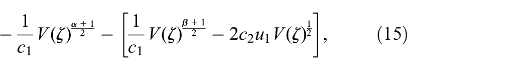
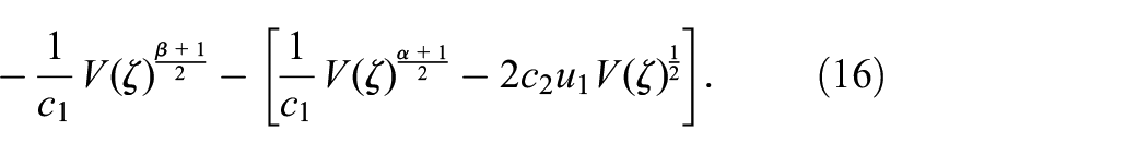
Substituting (9) and (13) into (11), we have

\begin{matrix} \overset{\cdot}{V} (ζ) = \frac{\partial V}{\partial ζ} g (ζ) |_{σ = 0} + \frac{\partial V}{\partial ζ_{3}} σ \\ \leq \frac{\partial V}{\partial ζ} g (ζ) |_{σ = 0} + ‖ \frac{\partial V}{\partial ζ_{3}} ‖ ‖ σ ‖ \\ \leq - \frac{1}{c_{1}} [V {(ζ)}^{\frac{d_{V_{0}} + d_{0}}{d_{V_{0}}}} + V {(ζ)}^{\frac{d_{V_{\infty}} + d_{\infty}}{d_{V_{\infty}}}}] + 2 c_{2} u_{1} V (ζ)^{\frac{1}{2}} \\ = - \frac{1}{c_{1}} [V {(ζ)}^{\frac{α + 1}{2}} + V {(ζ)}^{\frac{β + 1}{2}}] + 2 c_{2} u_{1} V (ζ)^{\frac{1}{2}} . \end{matrix}

(14)

For the convenience of the following discussion, the right side of inequality (14) can be rewritten as

- \frac{1}{c_{1}} V (ζ)^{\frac{α + 1}{2}} - [\frac{1}{c_{1}} V {(ζ)}^{\frac{β + 1}{2}} - 2 c_{2} u_{1} V {(ζ)}^{\frac{1}{2}}],

(15)

- \frac{1}{c_{1}} V (ζ)^{\frac{β + 1}{2}} - [\frac{1}{c_{1}} V {(ζ)}^{\frac{α + 1}{2}} - 2 c_{2} u_{1} V {(ζ)}^{\frac{1}{2}}] .

(16)

Also, by simple calculation we can obtain

\frac{1}{c_{1}} V (ζ)^{\frac{β + 1}{2}} - 2 c_{2} u_{1} V (ζ)^{\frac{1}{2}} > 0 \Leftrightarrow V (ζ) > (2 c_{1} c_{2} u_{1})^{\frac{2}{β}} : = Δ_{1},

\frac{1}{c_{1}} V (ζ)^{\frac{α + 1}{2}} - 2 c_{2} u_{1} V (ζ)^{\frac{1}{2}} > 0 \Leftrightarrow V (ζ) > (2 c_{1} c_{2} u_{1})^{\frac{2}{α}} : = Δ_{2} .

For convenience, let us continue the discussion in two cases.

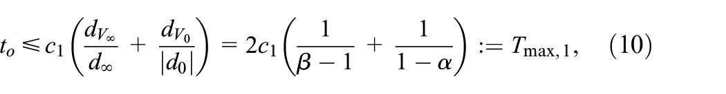
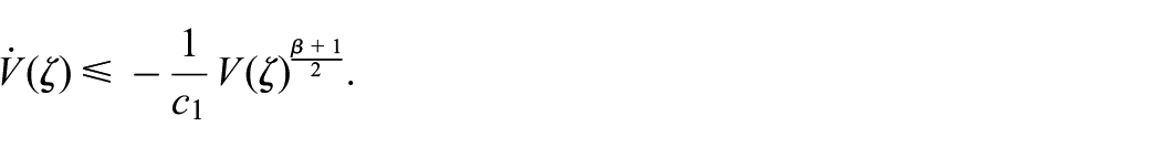
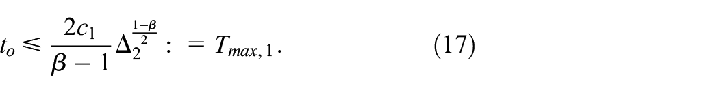
Case 1: Let $2 c_{1} c_{2} u_{1} \geq 1$ , then $Δ_{2} \geq Δ_{1} \geq 1$ .

Assuming that $V (ζ) > Δ_{2}$ , and on the basis of (14) and (16) we obtain

\overset{\cdot}{V} (ζ) \leq - \frac{1}{c_{1}} V (ζ)^{\frac{β + 1}{2}} .

Therefore, all solutions of $\overset{\cdot}{ζ} = g (ζ)$ converge to $O_{1}$ within a time $t_{o}$ , where

O_{1} = {ζ \in R^{6} | V (ζ) \leq Δ_{2}}

and

t_{o} \leq \frac{2 c_{1}}{β - 1} Δ_{2}^{\frac{1 - β}{2}} : = T_{\max, 1} .

(17)

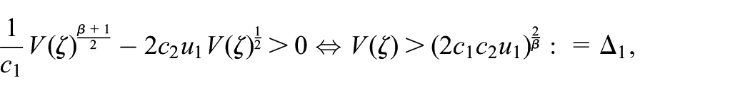
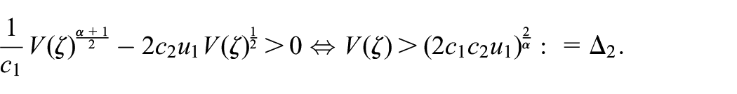
Case 2: Let $2 c_{1} c_{2} u_{1} < 1$ , then $0 < Δ_{2} < Δ_{1} < 1$ . From (14)–(16), we have

\overset{\cdot}{V} (ζ) \leq {\begin{matrix} - \frac{1}{c_{1}} V (ζ)^{\frac{β + 1}{2}}, V (ζ) \geq 1, \\ - \frac{1}{c_{1}} V (ζ)^{\frac{α + 1}{2}}, Δ_{1} < V (ζ) < 1 . \end{matrix}

Therefore, all solutions of $\overset{\cdot}{ζ} = g (ζ)$ first converge to

{ζ \in R^{6} | V (ζ) = 1}

within a time

t_{1} \leq \frac{2 c_{1}}{β - 1} : = T_{1},

and then, converge to $O_{2}$ within a time $t_{2}$ , where

O_{2} = {ζ \in R^{6} | V (ζ) \leq Δ_{1}}

and

t_{2} \leq \frac{2 c_{1}}{1 - α} (1 - Δ_{1}^{\frac{1 - α}{2}}) : = T_{2} .

Thus, the total converging time $t_{o}$ from the initial state to $O_{2}$ satisfies

t_{o} \leq T_{1} + T_{2} = \frac{2 c_{1}}{β - 1} + \frac{2 c_{1}}{1 - α} (1 - Δ_{1}^{\frac{1 - α}{2}}) : = T_{\max, 1} .

(18)

Hence, the conclusions of Theorem 1 hold.

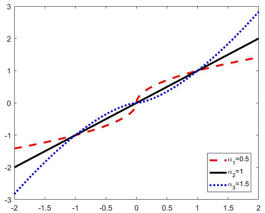
Remark 1: Observing the curves of the function $f_{i} (x) = Si g^{α_{i}} (x)$ ( $i = 1, 2, 3$ ) in Figure 3, where $α_{1} = 0.5$ , $α_{2} = 1$ , $α_{3} = 1.5$ , and it can be found that, when $| x | < 1$ the low-order power function $Si g^{0.5} (x)$ enlarges the signal $| x |$ , while the high-order power function $Si g^{1.5} (x)$ reduces it. However, they have the reverse property when $| x | \geq 1$ . Thus, the bi-limit-weighted function

f (x) = Si g^{α} (x) + Si g^{β} (x), 0 < α < 1, β > 1,

Figure 3.

Plots of $f_{i} (x) = Si g^{α_{i}} (x)$ .

can ensure that, when $| x | < 1$ the low-order power term $Si g^{α} (x)$ is dominant, while when $| x | \geq 1$ the high-order power term $Si g^{β} (x)$ is dominant. In this way, the FxTDO in (6) enlarges the estimation errors in the whole convergence process, resulting in faster transient speed.

Fixed-time inverse dynamics tracking control

In this section, a FxTIDTC scheme for the two-link manipulator in (1) will be designed. For this purpose, it is necessary to assume that $θ$ and $\overset{\cdot}{θ}$ are available from measurements.

The tracking errors $e = [e_{1}, e_{2}]^{T}$ and $\overset{\cdot}{e} = [{\overset{\cdot}{e}}_{1}, {\overset{\cdot}{e}}_{2}]^{T}$ are defined as

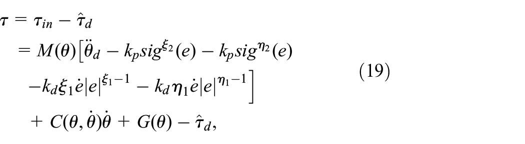
e = θ - θ_{d}, \overset{\cdot}{e} = \overset{\cdot}{θ} - {\overset{\cdot}{θ}}_{d} .

Then, the FxTIDTC law is proposed as

\begin{matrix} τ = τ_{in} - {\hat{τ}}_{d} \\ = M (θ) [{\overset{\cdot\cdot}{θ}}_{d} - k_{p} si g^{ξ_{2}} (e) - k_{p} si g^{η_{2}} (e) \\ - k_{d} ξ_{1} \overset{\cdot}{e} | e |^{ξ_{1} - 1} - k_{d} η_{1} \overset{\cdot}{e} | e |^{η_{1} - 1}] \\ + C (θ, \overset{\cdot}{θ}) \overset{\cdot}{θ} + G (θ) - {\hat{τ}}_{d}, \end{matrix}

(19)

in which $τ_{in}$ is the actual input torque, ${\hat{τ}}_{d}$ can be obtained by the FxTESDO in (6), and the parameters can be designed in the following development.

Case 3: The gains $k_{p}$ and $k_{d}$ are all positive real constants, so the following matrix $A_{2}$ is Hurwitz

A_{2} = [\begin{matrix} - k_{d} I I \\ - k_{p} I O \end{matrix}] .

Case 4: For $i = 1, 2$ , the exponents $ξ_{i}$ and $η_{i}$ are designed as those by Basin et al. (2017)

{\begin{matrix} ξ_{i} = i ξ - (i - 1), \\ η_{i} = i η - (i - 1), \end{matrix}

where $ξ \in (1 - 1 / 2, 1)$ , $η \in (1, 1 + 1 / 2)$ .

Denoting ${\tilde{τ}}_{d} = {\hat{τ}}_{d} - τ_{d}$ , and substituting (19) into (1), we obtain the following equation

\overset{\cdot\cdot}{e} + k_{p} si g^{ξ_{2}} (e) + k_{p} si g^{η_{2}} (e) + k_{d} ξ_{1} \overset{\cdot}{e} | e |^{ξ_{1} - 1}

+ k_{d} η_{1} \overset{\cdot}{e} | e |^{η_{1} - 1} + M^{- 1} (θ) {\tilde{τ}}_{d} = 0 .

(20)

Now, the design and analysis of the FxTIDTC in (19) can be summarized as a theorem in the following.

Theorem 2: For the two-link manipulator in (1), the FxTIDTC law designed in (19) based on the FxTESDO in (6), in which the design of parameters $ξ_{i}$ , $η_{i}$ , $k_{p}$ and $k_{d}$ satisfies the conditions (C3) and (C4), is given, and the controlled system is fixed-time stable tracking. More precisely, if $τ_{d} = 0$ (or ${\tilde{τ}}_{d} = 0$ ), the tracking error $[e, \overset{\cdot}{e}]^{T}$ uniformly converges to the origin within a time $t_{τ}$ upper bounded by $T_{\max, 2}$ which is independent of the initial conditions. Otherwise, if ${\tilde{τ}}_{d} \neq 0$ , the tracking error $[e, \overset{\cdot}{e}]^{T}$ uniformly converges to $O_{3}$ within $t_{τ} \leq T_{\max, 2}$ , where $O_{3}$ is a neighborhood of the origin.

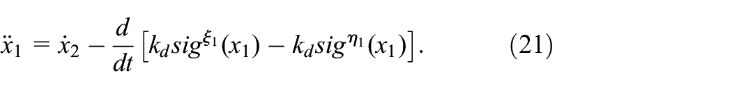
Proof: Define $x_{1} = e$ and introduce an intermediate variable $x_{2}$ , then, we have

{\overset{\cdot}{x}}_{2} = - k_{p} si g^{ξ_{2}} (x_{1}) - k_{p} si g^{η_{2}} (x_{1}) - M^{- 1} (θ) {\tilde{τ}}_{d},

and (20) can be rewritten as

{\overset{\cdot\cdot}{x}}_{1} = {\overset{\cdot}{x}}_{2} - \frac{d}{dt} [k_{d} si g^{ξ_{1}} (x_{1}) - k_{d} si g^{η_{1}} (x_{1})] .

(21)

By integrating both sides of equation (21), we obtain

{\begin{matrix} {\overset{\cdot}{x}}_{1} = x_{2} - k_{d} si g^{ξ_{1}} (x_{1}) - k_{d} si g^{η_{1}} (x_{1}), \\ {\overset{\cdot}{x}}_{2} = - k_{p} si g^{ξ_{2}} (x_{1}) - k_{p} si g^{η_{2}} (x_{1}) - M^{- 1} (θ) {\tilde{τ}}_{d} . \end{matrix}

(22)

According to Theorem 1 and equation (2), we have

∥ M^{- 1} (θ) {\tilde{τ}}_{d} ∥ \leq u_{2}, \forall t \geq T_{\max, 1},

where $u_{2}$ is a positive real constant.

By comparing the error systems (8) and (22), it is not hard to find that we can follow the ideas and methods of proving Theorem 1 to reach the following conclusions:

(1) Supposing $τ_{d} = 0$ (or ${\tilde{τ}}_{d} = 0$ ), all the solutions of system (22) converge to the origin within a time $t_{τ}$ which has

t_{τ} \leq 2 c_{3} (\frac{1}{η - 1} + \frac{1}{1 - ξ}) : = T_{\max, 2},

where $c_{3}$ is a positive real constant.

(2) Supposing that $τ_{d} \neq 0$ and ${\overset{\cdot}{τ}}_{d}$ is bounded, all the solutions of system (22) converge to $O_{3}$ within a time $t_{τ}$ . In detail, there exists a positive real constant $c_{4}$ and a Lyapunov function $V_{τ} (x)$ (where $x = [x_{1}, x_{2}]^{T}$ ) of system (22). Denote

Δ_{3} = (2 c_{3} c_{4} u_{2})^{\frac{2}{η}}, Δ_{4} = (2 c_{3} c_{4} u_{2})^{\frac{2}{ξ}} .

If $2 c_{3} c_{4} u_{2} \geq 1$ , we have

O_{3} = {x \in R^{4} | V_{τ} (x) \leq Δ_{4}}

and

t_{τ} \leq \frac{2 c_{3}}{η - 1} Δ_{4}^{\frac{1 - η}{2}} + T_{\max, 1} : = T_{\max, 2} .

If $2 c_{3} c_{4} u_{2} < 1$ , we have

O_{3} = {x \in R^{4} | V_{τ} (x) \leq Δ_{3}}

and

t_{τ} \leq \frac{2 c_{3}}{η - 1} + \frac{2 c_{3}}{1 - ξ} (1 - {Δ_{3}}^{\frac{1 - ξ}{2}}) + T_{\max, 1} : = T_{\max, 2} .

Hence, the conclusions of Theorem 1 hold.

Remark 2: It is not difficult to find that, the fixed-time control (let $τ = τ_{in}$ in (??)) can be realized even without FxTESDO, as long as $τ_{d}$ is bounded.

Remark 3:. It is undeniable that, the estimation of the upper bound $T_{\max, 2}$ is conservative, and the actual tracking time may be far less than $T_{\max, 2}$ . Nevertheless, it is noted that $T_{\max, 2}$ only depends on the parameters $ξ$ , $η$ , $α$ , $β$ , $c_{i}$ ( $i = 1, 2, 3, 4$ ) ( $c_{i}$ depends on the selected gains $k_{i}$ ( $i = 1, 2, 3$ ), $k_{p}$ , $k_{d}$ and Lyapunov functions V, $V_{τ}$ ), and two upper bounds $u_{1}$ , $u_{2}$ which can be obtained, which is conducive to controller design, because the tracking time can be adjusted to approach the requirement of engineering tasks.

Simulation studies

In this section, numerical simulation is employed to illustrate the effectiveness of the proposed FxTIDTC.

The parameters of system (1) are given by Zheng and Chen (2018) in SI units: $m_{1} = 2.148$ kg, $m_{2} = 0.114$ kg, $l_{1} = 0.100$ m, $l_{2} = 0.255$ m, and $g = 9.8$ $N / kg$ . The expected tracking signal is set as $θ_{d} = [\cos (t), \sin (t)]^{T}$ (rad). The control law in system (1) is given by the FxTIDTC in (??), and the external disturbance is estimated by the FxTESDO in (6).

An external time-varying disturbance is described by $τ_{d} = [0.2 \sin (t), 0.2 \cos (t)]^{T}$ ( $N \cdot m$ ). The initial conditions of the joint positions and velocities are $θ = [1.5, 1.5]^{T}$ and $\overset{\cdot}{θ} = [0, 0]^{T}$ (rad).

The gains and exponents of the FxTIDTC in (19) are chosen by trial-and-error

ξ = 0.7, η = 1.3, k_{p} = 36, k_{d} = 12 .

(23)

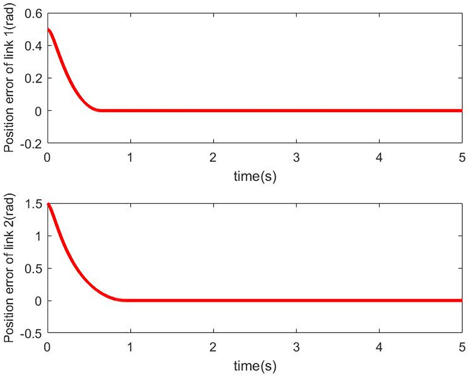
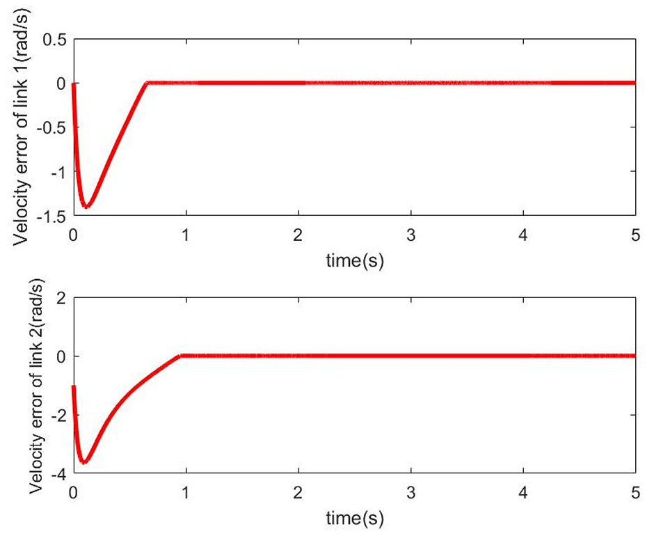
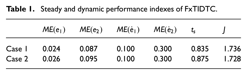
First of all, in the case $τ_{d} = 0$ in (1), the position and velocity tracking errors of the FxTIDTC are shown in Figure 4 and Figure 5, respectively. Steady and dynamic performance indexes for the controller are also given in Case 1 of Table 1, in which $ME (\cdot) = \int_{0}^{t} | \cdot | dt / t$ denotes the mean error and $t = 5$ , $t_{s}$ is the setting time defined as follows

t_{s} = \max {t_{s, 1}, t_{s, 2}},

where

t_{s, i} = \min {T : | e_{i} (t) | \leq 0.2 | θ_{d, i} (t) |, \forall t \geq T},

Figure 4.

Position tracking errors of FxTIDTC.

Figure 5.

Velocity tracking errors of FxTIDTC.

Table 1.

Steady and dynamic performance indexes of FxTIDTC.

	$ME (e_{1})$	$ME (e_{2})$	$ME ({\overset{\cdot}{e}}_{1})$	$ME ({\overset{\cdot}{e}}_{2})$	$t_{s}$	J
Case 1	0.024	0.087	0.100	0.300	0.835	1.736
Case 2	0.026	0.095	0.100	0.300	0.875	1.728

and $J = \int_{0}^{t_{s}} τ^{T} (t) τ (t) dt$ denotes the control energy required to make the system reach the equilibrium state. As we can see in Figures 4–5 and Case 1 of Table 1, the FxTIDTC can ensure the correctness of trajectory tracking in a short time.

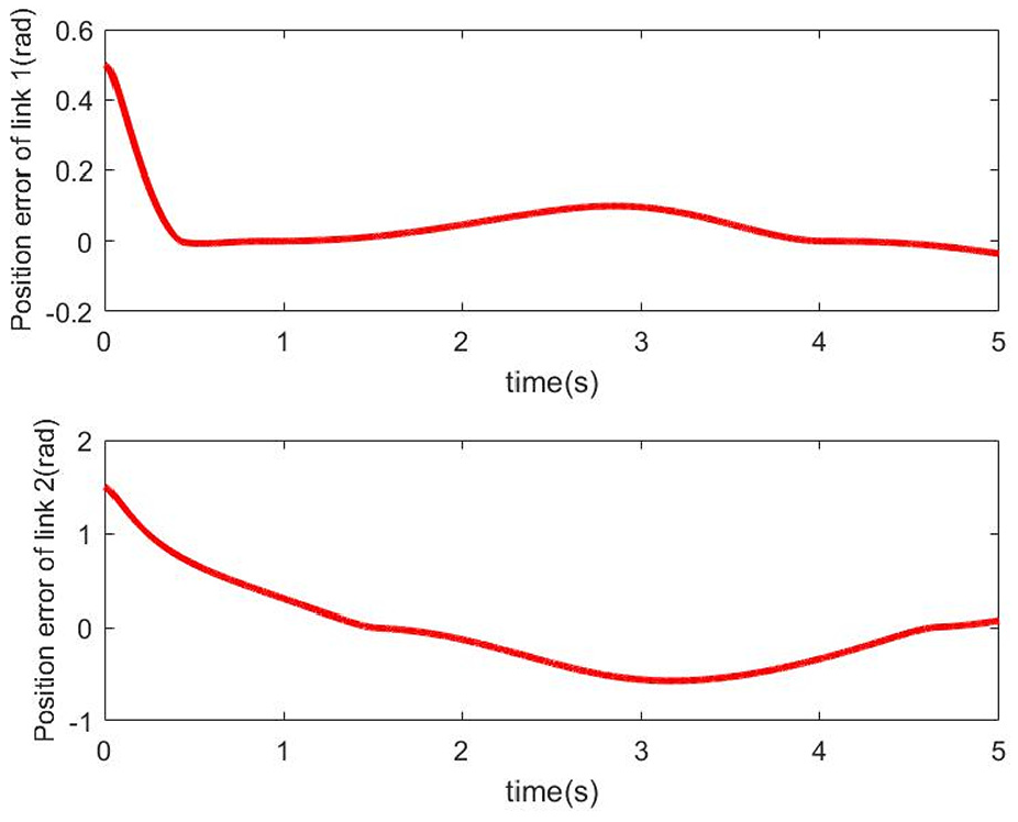
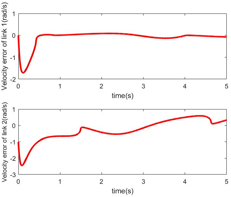
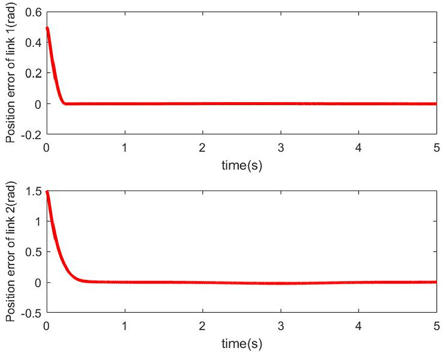
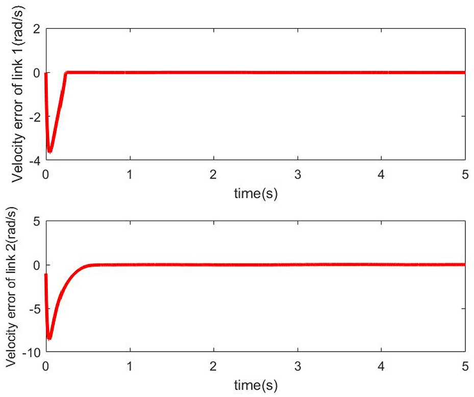
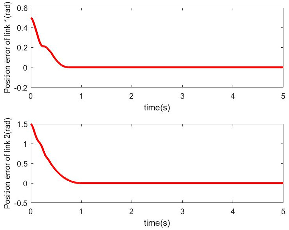
When the system is under external disturbance $τ_{d}$ , the tracking performance of the FxTIDTC is reduced, as shown in Figures 6–7. Let us enlarge the gains of the FxTIDTC to $k_{p} = 225$ , $k_{d} = 30$ , and plot the position and velocity tracking errors of FxTIDTC, as shown in Figures 8–9. As we can see, the FxTIDTC can achieve better robustness based on the large gains.

Figure 6.

Position tracking errors under disturbance.

Figure 7.

Velocity tracking errors under disturbance.

Figure 8.

Position errors of FxTIDTC under large gains.

Figure 9.

Velocity errors of FxTIDTC under large gains.

To ensure excellent tracking performance under small gains in (23), we introduce the FxTESDO (6) whose parameters are selected as

α = 0.7, β = 1.3, k_{1} = 40, k_{2} = 130, k_{3} = 10 .

Since $λ_{M} = 246.17$ , the selected gains satisfy $k_{1} k_{2} > 2 k_{3} λ_{M}$ . The position and velocity tracking errors are shown in Figures 10–11. Steady and dynamic performance indexes for the controller are also given in Case 2 of Table 1.

Figure 10.

Position errors of FxTIDTC based on FxTESDO.

Figure 11.

Velocity errors of FxTIDTC based on FxTESDO.

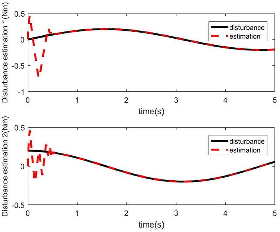
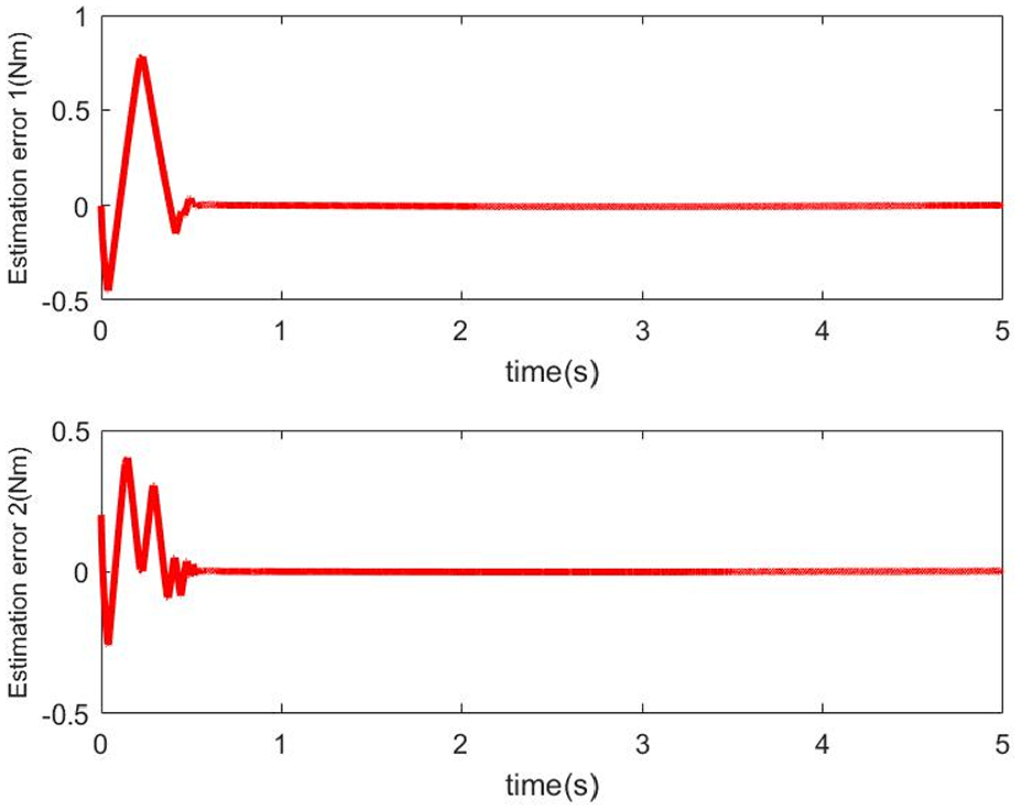
From Figures 10–11 and Case 2 of Table 1, it can be seen that the controlled system with FxTESDO has excellent tracking performance. The estimation curves of external disturbance and estimation errors are shown in Figures 12–13, indicating that the FxTESDO can quickly estimate external disturbances as long as the appropriate parameters are selected.

Figure 12.

Disturbances $τ_{d 1}, τ_{d 2}$ and their estimated values.

Figure 13.

Estimation errors of FxTESDO.

Conclusions

For a two-link manipulator, we have addressed the fixed-time tracking problem based on the fixed-time estimation of external disturbances. The control goal has been achieved by modifying the ESO and inverse dynamics control. The designed FxTESDO can realize fixed-time estimation of external disturbances, and the proposed FxTIDTC can perform fixed-time tracking, which have been proved with the Lyapunov’s direct method and the bi-limit homogeneous technique. Numerical simulations have illustrated that the proposed FxTIDTC has fast transient performance and good robustness. This paper has not only provided a theoretical basis for the robustness of FxTC against external disturbances, but also offered an improved design for faster disturbance estimation and high-accuracy trajectory tracking of manipulators. However, this paper does not consider the modeling uncertainty in system (1), so we will explore the use of Taylor network to deal with this problem in the following research.

Footnotes

Appendix A

Denote $λ_{1} (θ)$ and $λ_{2} (θ)$ as the eigenvalues of $M^{- 1} (θ)$ . Since the matrix $M^{- 1} (θ)$ is positive definite for all joint position $θ$ , we have

λ_{1} (θ) > 0, λ_{2} (θ) > 0, | M^{- 1} | = λ_{1} (θ) λ_{2} (θ) > 0,

0 < 2 λ_{m} \leq tr (M^{- 1}) = λ_{1} (θ) + λ_{2} (θ) \leq 2 λ_{M},

and

Ξ_{1} = t r^{2} (M^{- 1}) - 4 | M^{- 1} | = [λ_{1} (θ) - λ_{2} (θ)]^{2} \geq 0 .

The eigenpolynomial of $A_{1}$ is

a_{6} s^{6} + a_{5} s^{5} + a_{4} s^{4} + a_{3} s^{3} + a_{2} s^{2} + a_{1} s + a_{0},

in which

a_{6} = 1, a_{5} = 2 k_{1}, a_{4} = k_{1}^{2} + 2 k_{2},

a_{3} = 2 k_{1} k_{2} + k_{3} tr (M^{- 1}), a_{2} = k_{2}^{2} + k_{1} k_{3} tr (M^{- 1}),

a_{1} = k_{2} k_{3} tr (M^{- 1}), a_{0} = k_{3}^{2} | M^{- 1} | .

Obviously a_{i} > 0 (i = 1, 2, \dots, 6) and

Ξ_{2} = k_{1} k_{2} - k_{3} tr (M^{- 1}) > 0

if $k_{i} > 0$ $(i = 1, 2, 3)$ and $k_{1} k_{2} > 2 k_{3} λ_{M}$ .

Let us make the Routh array table as follows.

In Table 2, there have

b_{1} = - \frac{1}{a_{5}} | \begin{matrix} a_{6} \\ a_{5} \end{matrix} \begin{matrix} a_{4} \\ a_{3} \end{matrix} | = \frac{b_{11}}{a_{5}} = \frac{2 k_{1}^{3} + k_{1} k_{2} + Ξ_{2}}{a_{5}} > 0,

j_{1} = - \frac{1}{b_{1}} | \begin{matrix} a_{5} \\ a_{1} \end{matrix} \begin{matrix} a_{3} \\ a_{2} \end{matrix} | = \frac{j_{11}}{b_{11}}

= \frac{(k_{1} k_{2} + Ξ_{2}) [2 k_{1}^{3} + k_{3} tr (M^{- 1})]}{b_{11}} > 0,

l_{1} = - \frac{1}{b_{1}} | \begin{matrix} b_{1} \\ j_{1} \end{matrix} \begin{matrix} b_{2} \\ j_{2} \end{matrix} | = \frac{k_{1} l_{11}}{j_{11}}

where

\begin{matrix} l_{11} = Ξ_{2} [k_{3}^{2} t r^{2} (M^{- 1}) + 2 k_{1}^{3} k_{3} tr (M^{- 1}) + 2 k_{3}^{2} | M^{- 1} | \\ + 4 k_{1} k_{2} Ξ_{2}] + 2 k_{1} k_{3}^{2} | M^{- 1} | (2 k_{1}^{2} + k_{2}) > 0, \end{matrix}

q_{1} = - \frac{1}{l_{1}} | \begin{matrix} j_{1} \\ l_{1} \end{matrix} \begin{matrix} j_{2} \\ l_{2} \end{matrix} | = \frac{q_{11}}{l_{11}},

and

q_{11} = (k_{1} k_{2} Ξ_{2} + k_{3}^{2} | M^{- 1} |) [4 k_{1} k_{2} tr (M^{- 1}) Ξ_{2}

+ 2 k_{1}^{3} k_{3} Ξ_{1} + k_{3}^{2} t r^{3} (M^{- 1})] > 0,

w_{1} = - \frac{1}{q_{1}} | \begin{matrix} l_{1} \\ q_{1} \end{matrix} \begin{matrix} l_{2} \\ 0 \end{matrix} | = k_{3}^{2} | M^{- 1} | > 0 .

Therefore, $A_{1}$ is Hurwitz stable according to the Routh-Hurwitz Criterion.

Declaration of conflicting interests

The author(s) declared no potential conflicts of interest with respect to the research, authorship, and/or publication of this article.

Funding

The author(s) disclosed receipt of the following financial support for the research, authorship, and/or publication of this article: This research was supported in part by the Key R & D projects (Social Development) in Jiangsu Province of China under Grant BE2020704, in part by Jiangsu Province “333” project under Grant BRA2019051, in part by the Development Program of the Higher Education Institutions in Shandong Province under Grant J17KB120, and in part by the Research Fund of Binzhou University under Grant BZXYG1701.

ORCID iD

Heli Gao

References

Andrieu

Praly

Astolﬁ

(2008) Homogeneous approximation, recursive observer design, and output feedback. SIAM Journal on Control and Optimization 47(4): 1814–1850.

Baek

Jin

Han

(2016) A new adaptive sliding-mode control scheme for application to robot manipulators. IEEE Transactions on Industrial Electronics 63(6): 3628–3637.

Basin

Shtessel

(2017) Finite-and ﬁxed-time differentiators utilising HOSM techniques. IET Control Theory & Applications 11(8): 1144–1152.

Bernuau

Eﬁmov

Perruquetti

Polyakov

(2014) On homogeneity and its application in sliding mode control. Journal of the Franklin Institute 351(4): 1866–1901.

Bhat

Bernstein

(1997) Finite-time stability of homogeneous systems. In: Proceedings of the American Control Conference, Albuquerque, NM, USA, 04–06 Jun 1997, pp. 2513–2514. IEEE

Bhat

Bernstein

(2000) Finite-time stability of continuous autonomous systems. SIAM Journal on Control and Optimization 38(3): 751–766.

Cao

Zou

Jia

, et al. (2019) RRT-based path planning for an intelligent litchi-picking manipulator. Computers and Electronics in Agriculture 156(2019): 105–118.

Chen

Selvaggio

Caldwell

(2019) Dexterous grasping by manipulability selection for mobile manipulator with visual guidance. IEEE Transactions on Industrial Informatics 15(2): 1202–1210.

Chen

(2013) Direct adaptive neural control for a class of uncertain nonafﬁne nonlinear systems based on disturbance observer. IEEE Transactions on Cybernetics 43(4): 1213–1225.

10.

Chen

(2004) Disturbance observer-based control for nonlinear systems. IEEE/ASME Transactions on Mechatronics 9(4): 706–710.

11.

Chen

Ballance

Gawthrop

O’Reilly

(2000) A nonlinear disturbance observer for robotic manipulators. IEEE Transactions on Industrial Electronics 47(4): 932–938.

12.

Chen

Huang

Sun

, et al. (2020a) RBF-neural-network-based adaptive robust control for nonlinear bilateral teleoperation manipulators with uncertainty and time delay. IEEE/ASME Transactions on Mechatronics 25(2): 906–918.

13.

Chen

Huang

Yang

Yao

(2020b) Adaptive fuzzy backstepping control for stable nonlinear bilateral teleoperation manipulators with enhanced transparency performance. IEEE Transactions on Industrial Electronics 67 (1): 746–756.

14.

Chiu

(2012) Derivative and integral terminal sliding mode control for a class of MIMO nonlinear systems. Automatica 48(2): 316–326.

15.

Ertugrul

Kaynak

(2000) Neuro sliding mode control of robotic manipulators. Mechatronics 10(2000): 239–263.

16.

Feng

Man

(2002) Non-singular terminal sliding mode control of rigid manipulators. Automatica 38(12): 2159–2167.

17.

Ferrara

Incremona

(2015) Design of an integral suboptimal second-order sliding mode controller for the robust motion control of robot manipulators. IEEE Transactions on Control Systems Technology 23(6): 2316–2325.

18.

Galicki

(2015) Finite-time control of robotic manipulators. Automatica 51(2015): 49–54.

19.

Galicki

(2016) Finite-time trajectory tracking control in a task space of robotic manipulators. Automatica 67(2016): 165–170.

20.

Gueaieb

Karray

Al-Sharhan

(2007) A robust hybrid intelligent position/force control scheme for cooperative manipulators. IEEE/ASME Transactions on Mechatronics 12(2): 109–125.

21.

Han

(2009) From PID to active disturbance rejection control. IEEE Transactions on Industrial Electronics 56 (3): 900–906.

22.

Han

Zheng

(2019) A non-decoupled backstepping control for ﬁxed-wing UAVs with multivariable ﬁxed-time sliding mode disturbance observer. Transactions of the Institute of Measurement and Control 41(4): 963–974.

23.

, et al. (2015) Neural network control of a rehabilitation robot by state and output feedback. Journal of Intelligent & Robotic Systems 80(1): 15–31.

24.

Hong

Huang

(2002) Finite-time control for robot manipulators. Systems & Control Letters 46(4): 243–253.

25.

Huang

Wang

Meng

, et al. (2016) Reconﬁgurable spacecraft attitude takeover control in post-capture of target by space manipulators. Journal of the Franklin Institute 353(2016): 1985–2008.

26.

Kawamura

Seno

Kobayashi

Ieiri

Hashizume

Gujie

(2016) Design parameter evaluation based on human operation for tip mechanism of forceps manipulator using surgical robot simulation. Advanced Robotics 30(7): 476–488.

27.

Kim

(2004) Output feedback tracking control of robot manipulators with model uncertainty via adaptive fuzzy logic. IEEE Transactions on Fuzzy Systems 12(3): 368–378.

28.

Kim

Rew

Kim

(2010) Disturbance observer for estimating higher order disturbances in time series expansion. IEEE Transactions on Automatic Control 55 (8): 1905–1911.

29.

Lee

Utkin

Malinin

(2009) Chattering reduction using multiphase sliding mode control. International Journal of Control 82(9): 1720–1737.

30.

Lin

Kuo

Wang

(2016) Grasping posture control design for a home service robot using an ABC-based adaptive PSO algorithm. International Journal of Advanced Robotic Systems 13(3): 118–132.

31.

Chen

Cai

(2018) Resilient control based on disturbance observer for nonlinear singular stochastic hybrid system with partly unknown Markovian jump parameters. Journal of the Franklin Institute 355(5): 2243–2265.

32.

Yang

Tang

(2013) Decentralised adaptive fuzzy control of coordinated multiple mobile manipulators interacting with non-rigid environments. IET Control Theory and Applications 7(3): 397–410.

33.

Liu

Chen

(2018) Fixed-time disturbance observer design for Brunovsky systems. IEEE Transactions on Circuits and Systems łII: Express Briefs 65(3): 341–345.

34.

Liu

, et al. (2017) Fast ﬁxed-time nonsingular terminal sliding mode control and its application to chaos suppression in power system. IEEE Transactions on Circuits and Systems łII: Express Briefs 64(2): 151–155.

35.

Patiño

Carelli

Kuchen

(2002) Neural networks for advanced control of robot manipulators. IEEE Transactions on Neural Networks 13(2): 343–354.

36.

Polyakov

(2012) Nonlinear feedback design for ﬁxed-time stabilization of linear control systems. IEEE Transactions on Automatic Control 57(8): 2106–2110.

37.

Polyakov

Fridman

(2014) Stability notions and Lyapunov functions for sliding mode control systems. Journal of the Franklin Institute 351(4): 1831–1865.

38.

Rosier

(1992) Homogeneous Lyapunov function for homogeneous continuous vector ﬁeld. Systems & Control Letters 19(6): 467–473.

39.

Spong

Hutchinson

Vidyasagar

(2004) Robot Dynamics and Control. New York: Wiley.

40.

(2009) Global continuous ﬁnite-time tracking of robot manipulators. International Journal of Robust and Nonlinear Control 19(17): 1871–1885.

41.

Zheng

(2019) Fixed-time inverse dynamics control for robot manipulators. Journal of Dynamic Systems, Measurement, and Control 141(6): 1814–1850.

42.

Sun

(2019) Augmented ﬁxed-time observer-based continuous robust control for hypersonic vehicles with measurement noises. IET Control Theory and Applications 13(3): 422–433.

43.

Sun

Wang

(2005) A robust robotic tracking controller based on neural network. International Journal of Robotics & Automation 20(3): 199–204.

44.

Tian

Zuo

Yan

Wang

(2017) A ﬁxed-time output feedback control scheme for double integrator system. Automatica 80 (11): 17–24.

45.

Trujillo

MÁ

Martínez-de Dios

Martín

, et al. (2019) Novel aerial manipulator for accurate and robust industrial NDT contact inspection: a new tool for the oil and gas inspection industry. Sensors 19(6): 1305.

46.

Venkataraman

Gulati

(1993) Control of nonlinear systems using terminal sliding modes. Journal of Dynamic Systems, Measurement, and Control 115(3): 554–560.

47.

Wang

Chai

Zhai

(2009) Neural-network-based terminal sliding-mode control of robotic manipulators including actuator dynamics. IEEE Transactions on Industrial Electronics 56 (9): 3296–3304.

48.

Wei

Yang

, et al. (2017) FxTDO-based non-singular terminal sliding mode control for second-order uncertain systems. IET Control Theory & Applications 12(18): 2459–2467.

49.

Yang

Wei

Cui

(2018) Non-recursive ﬁxed-time convergence observer and extended state observer IEEE Access 6(2018): 62339–62351.

50.

Yang

(2013) Continuous nonsingular terminal sliding mode control for systems with mismatched disturbances. Automatica 49(7): 2287–2291.

51.

Yang

(2011) Nonsingular fast terminal sliding-mode control for nonlinear dynamical systems. International Journal of Robust and Nonlinear Control 21(16): 1865–1879.

52.

Yang

Tsubakihara

Kanae

, et al. (2008) A novel robust nonlinear motion controller with disturbance observer. IEEE Transactions on Control Systems Technology 16(1): 137–147.

53.

Zhang

(2017) Fixed-time regulation control of uncertain nonholonomic systems and its applications. International Journal of Control 90(7): 1327–1344.

54.

Zheng

Chen

(2018) Tracking control of manipulator based on high-order disturbance observer. IEEE Access 6(2018): 26753–26764.

55.

Zuo

(2015a) Non-singular ﬁxed-time terminal sliding mode control of non-linear systems. IET Control Theory and Applications 9(4): 545–552.

56.

Zuo

(2015b) Non-singular ﬁxed-time consensus tracking for second-order multi-agent networks. Automatica 54(2015): 305–309.