
Abstract
Simultaneous investigation of demand response programs and false data injection cyber-attack are critical issues for the smart power system frequency regulation. To this purpose, in this paper, the output of the studied system is simultaneously divided into two subsystems: one part including false data injection cyder-attack and another part without cyder-attack. Then, false data injection cyber-attack and load disturbance are estimated by a non-linear sliding mode observer, simultaneously and separately. After that, demand response is incorporated in the uncertain power system to compensate the whole or a part of the load disturbance based on the available electrical power in the aggregators considering communication time delay. Finally, active disturbance rejection control is modified and introduced to remove the false data injection cyber-attack and control the uncompensated load disturbance. The salp swarm algorithm is used to design the parameters. The results of several simulation scenarios indicate the efficient performance of the proposed method.
Keywords
Introduction
Intelligent power systems with their non-negligible advantages are replacing the conventional forms. These intelligent systems have a series of functions including generation, consumption, a balance between them, and protection, which are regulated by the control center. Since, during the entire process of intelligent power systems, signals are sent to control the generation and consumption units, the infrastructure of an intelligent power system must be based on the communication systems. However, this feature may make them vulnerable to false data injection cyber-attack (FDICA). Attackers tend to disrupt the intelligent power system operation by manipulating and delaying the transferred and measured data (Li et al., 2018; Sargolzaei et al., 2016; Shafique and Iqbal, 2015), denying of service (Liu et al., 2013; Shen et al., 2019), or replacing the corrected data with false data (Abbaspour et al., 2017; Ameli et al., 2018; Chen et al., 2018; Huang et al., 2018; Khalaf et al. 2019; Law et al., 2015; Mohajerin Esfahani et al., 2010; Sargolzaei et al., 2017; Zhang and Li 2017).
Under FDICA conditions, incorrect data are designed to dominate the control center, causing an operator to send wrong commands to the generation units so that the balance between the generated power and the consumed load is disturbed. As a result, while the power system frequency is either increasing or decreasing, the trip command from the frequency relays is issued. In contrast to FDICA, the first step is detection and diagnosis of the attack location and significance. Among recent studies, an unknown input observer has been employed to identify FDICA without predicting the load changes (Ameli et al., 2018). The accuracy of unknown input observer depends on adequate knowledge of the studied system and optimal selection of the time delay. In addition, the reachability methods (Mohajerin Esfahani et al., 2010), an algorithm based on dynamic watermarking (Huang et al., 2018), simultaneous input and state estimation–based algorithms (Law et al., 2015), and the game-theoretic approach combining quantitative risk management techniques are some methods for the detection of FDICA (Abbaspour et al., 2017).
In Chen et al. (2018) and Khalaf et al. (2019), neural networks are used for FDICA detection. Since the neural networks–based methods are designed in compliance with previous data for estimating future outputs, their accuracy is about 90% (Zhang and Li, 2017). Also, cryptographic methods are not able to protect the system against cyber-attacks (Sargolzaei et al., 2017).
However, considering the ability of the intelligent power systems to manage the load side, demand response programs were developed to help the power system operation in keeping the frequency at the allowable range (Pourmousavi and Nehrir, 2014). When demand response is incorporated in the power system, generation units are not merely responsible anymore for the frequency regulation (Bao et al., 2017). It is worth mentioning that the load frequency control actions (related to decreasing or increasing the generated power) with the demand response programs are less than those without demand response programs. As a result, smooth operation is achieved (Singh et al., 2017). In demand response programs, the aggregators play an interface role between the operator and the customers. Aggregator contracts with the customers to keep their electricity available. Then, it sells the available energy to the operators. Incorporation of demand response into load frequency control leads to many advantages including increasing the stability of the system and the reachability of the electrical energy and decreasing costs and losses (Shiltz et al., 2019). Although every type of load can be involved in the demand response program, thermostatically controlled loads are more likely to be participated due to their characteristics (Samarakoon et al., 2012). To participate, the demand response in the power system, predictive control (Lampropoulos et al., 2013), the lazy state switching control mode (Chen et al., 2020), and hybrid hierarchical demand response control (Bao et al., 2015) have been designed. However, in these mentioned studies, there is a lacuna about how much power is required from the demand response Programs (PDR).
As discussed, in the demand response program, consumers make a significant contribution to the operation of an intelligent power system by changing their consumption during peak periods or whenever the operator commands them. To cope with this issue, the necessary infrastructure should be established to regulate the amount of power required from PDR (Babahajiani et al., 2018) and find out whether the available electrical power in the aggregators (PAGG) is able to supply the PDR or not. The PDR must be equal to load disturbance (LDS) to retain the frequency in the allowable range. Due to the unexpected characteristic of LDS, it seems the calculation of its actual amount is impossible. Therefore, there is an emptiness in dealing with these problems.
FDICA and LDS are the types of faults. The non-linear sliding mode observer has been designed for fault detection and reconstruction (Alwi et al., 2011; Edwards et al., 2000; Shtessel et al., 2014). If the state-space equation of the power system is extracted, the effect of FDICA places is observed on the output equations, and the effect of demand response participation is on the state equations. Therefore, for both FDICA detection and demand response participation in load frequency control, the system should be separated into two parts, one including FDICA without demand response programs and another part including demand response participation without FDICA. The decomposition methods or filtering the output methods can be applied to confront this problem. The decomposition methods are carried out based on singular value decomposition (Corless and Jay 1998; Raoufi and Marquezz, 2010) and the linear matrix inequality (Abdollahi, 2018). The filtering of the output methods is more accessible than the decomposition method, because the procedure of filtering design is easier. For fault detection and reconstruction, non-linear sliding mode observer has been used with both the decomposition methods (Chen and Chowdhury, 2010; Zhang et al., 2012) and the filtering of the output methods (Tan and Edwards, 2002, 2003).
The next step after fault detection is rejection or control them to keep the power system frequency at the stable conditions. Active disturbance rejection control with an extended state observer is a practical approach to remove the negative effect of disturbance in the presence of uncertainty and noise (Han, 2009). Active disturbance rejection control has been successfully applied to automatic generation control to regulate the power system frequency (Huang et al., 2019; Tan et al., 2015). Extended state observer cannot separate faults (e.g. FDICA from LDS(. Therefore, common active disturbance rejection control has some limitations in dealing with separating faults and accurate estimation.
According to the above discussions, there is a concern about the simultaneous investigation of cyber-attack tolerant and participation of the demand response program in the load frequency control. Therefore, this paper aims to find a simultaneous solution for an intelligent power system considering these fundamental issues due to the absence of investigation. To deal with these problems, some essential steps should be simultaneously adopted, including
Detecting the existence of the FDICA and reconstructing it;
Discovering the location of the FDICA;
Calculating the PDR and PAGG;
Finding out whether PAGG is able to supply the PDR;
Removing the FDICA and compensating the LDS.
The main contributions of this paper are presented as follows:
Presenting a new model for the automatic generation control under FDICA with the presence of the demand response program.
Modification of active disturbance rejection control by changing its structure and combining it with the non-linear sliding mode observer to detect and reconstruct FDICA and LDS simultaneously. Then, it removes the FDICA and controls the LDS.
Implementing the demand response program to compensate the whole or part of LDS based on the available power at the aggregators.
Optimization of the modified active disturbance rejection control and non-linear sliding mode observer by the salp swarm algorithm.
Proposing a novel algorithm based on non-linear sliding mode observer and modified active disturbance rejection control to control power system frequency under FDICA and participation of demand response conditions.
The structure of this paper is organized as follows: In “Modeling of automatic generation control under FDICA with the presence of demand response program” section, the modeling of automatic generation control under FDICA with the presence of the demand response program is provided. “Simultaneous detection and reconstruction of FDICA and demand response power” section presents the simultaneous detection and reconstruction of FDICA and demand response power by non-linear sliding mode observer. In “Removing FDICA and compensating the ULDS” section, the active disturbance rejection control is modified to remove FDICA and uncompensated load disturbance (ULDS). The analysis of stability in the proposed method is provided in “Stability analysis” section. In “The proposed algorithm” section, the proposed algorithm is explained. In “Results” section, simulation results from several scenarios have been given. Conclusions are available in the “Conclusion” section.
Modeling of automatic generation control under FDICA with the presence of demand response program
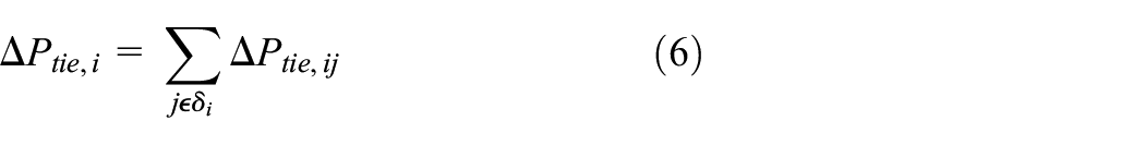
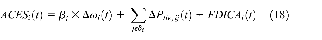
Automatic generation control has two primary responsibilities: maintaining the frequency in the acceptable range and controlling the transferred power between the areas (Bevrani, 2009). The structure of simple one controlling area has been shown in Figure 1. In the conventional power systems, automatic generation control performs these duties based on commanding to the generation units. But, in intelligent power systems, demand response programs are also involved in fulfilling these duties. The frequency and transferred power between areas deviate from the nominal values due to the load changes. Area control error signal is composed of the sum of those two deviations. Therefore, area control error signal deviates from the setpoint. The area control error signal is then sent to the control center. The control center sends proper commands to the generation units according to the area control error signal deviation. The generation units decrease or increase their electrical power generation in reaction to the control center commands (Wood Allen et al., 2013). The intelligent power system is comprised of many controlling areas. There are some generation units inside each area. These generation units are responsible for supplying the loads located inside of those areas. Furthermore, some of these generation units contribute to supplying the load in the neighborhood area in an emergency condition. Tie lines connect the areas.
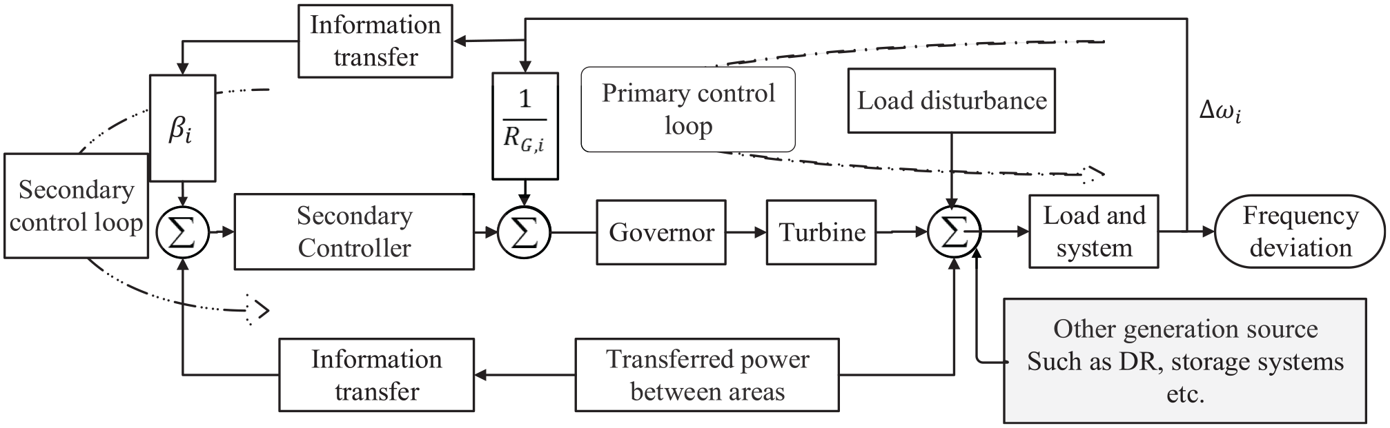
A simple one controlling area with one generation unit.
In the following, at first, in “The state-space model of automatic generation control” section, the state-space model of automatic generation control will be shown, then in “The state-space model of automatic generation control considering the demand response program and FDICA” section, the state-space model of automatic generation control considering demand response program and FDICA will be extracted. Comparing the state-space model in these sections will show where the demand response program and FDICA are placed in system modeling.
The state-space model of automatic generation control
The area control error signal in the ith controlling area is defined as in equation (1)

where
where
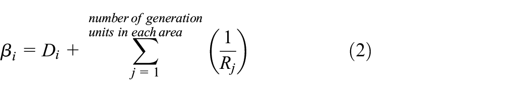
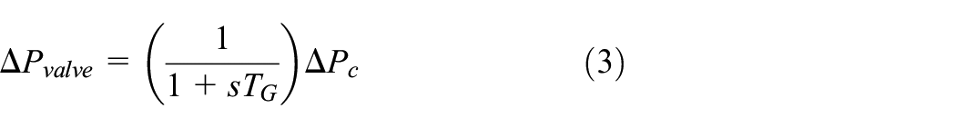
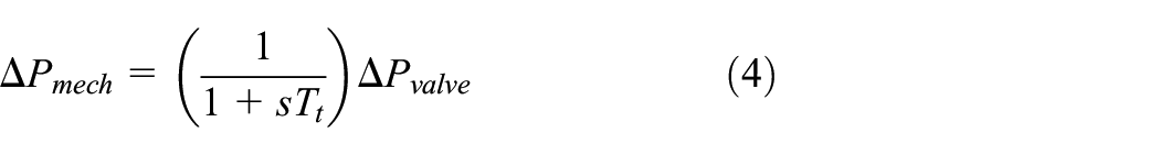
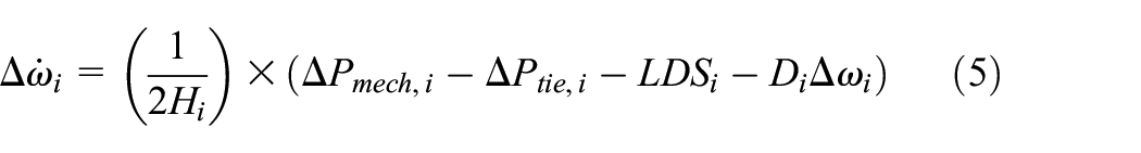
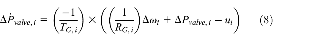
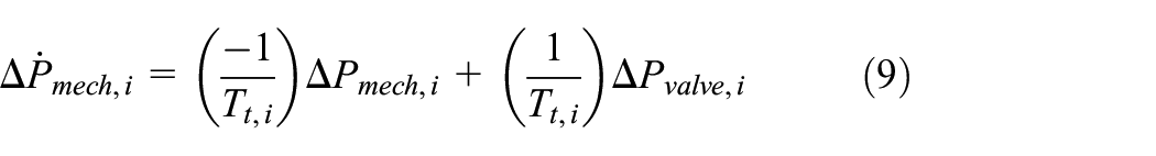
The state-space model of automatic generation control can be extracted considering Figure 1, the studied time horizon, and type and severity of the investigated fault at the automatic generation control studies. Some equipment of the power system can be ignored due to their faster or slower actions, and the linearization method can be used considering the mentioned factors. The governor and none-reheat turbine transfer function are defined as in equations (3) and (4)
where
where

where

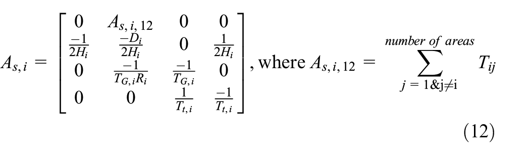
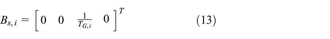
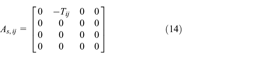
Increasing the number of generation units leads to increment of system states. Without considering the demand response program and FDICA, the state-space model of automatic generation control is obtained as in equation (11)
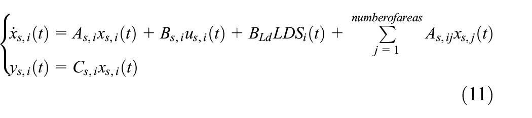
where
The system outputs are considered as
The state-space model of automatic generation control considering the demand response program and FDICA
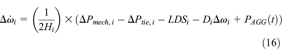
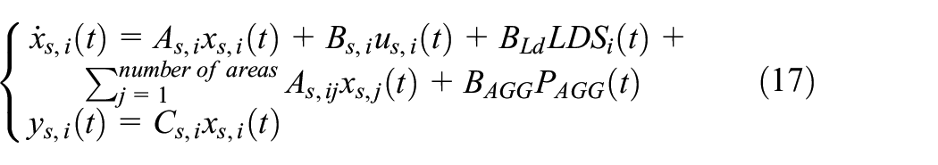
Like generation units, the demand response program injects the electrical power to the grid. As shown in Figure 1, the injected power by demand response is simulated as a virtual power plant. A virtual power plant in automatic generation control is considered parallel with the primary generation units. Therefore, the effect of demand response is evaluated at the state equations. With the demand response program participation in frequency regulation, the area control error signal is also sent to the aggregators. Considering area control error signal, the aggregators send commands to costumers to turn off or turn on their electrical appliances based on their contract with the costumers. Aggregators make the control center aware of how much is the PAGG. PAGG may be more significant than LDS or smaller than it. However, the problem is how much demand response power must be involved in the frequency regulation. This value is equal with the LDS. According to the effect of the demand response program, equation (5) changes to equation (16)
Considering the PAGG and determining LDS, generation units receive commands to compensate
where
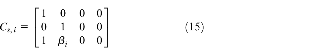
Since the area control error signal is an output of the automatic generation control, therefore, the effects of FDICA in automatic generation control appear in the system output equations. Considering FDICA, the mentioned state-space model of automatic generation control in equation (16) can be rewritten as equation (19)
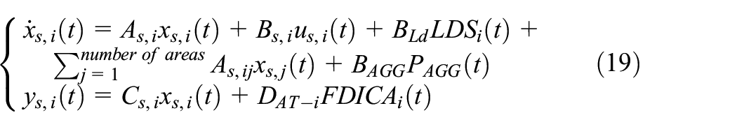
where

Since the main purpose of the demand response program is to compensate the LDS,
Simultaneous detection and reconstruction of FDICA and demand response power
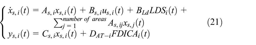
Inspired by the works presented in Edwards et al. (2000) and Tan and Edwards (2002), a non-linear sliding mode observer has been used in this paper to simultaneously detect and reconstruct FDICA and the PDR. Finding out the actual value of PDR is dependent upon the accurate estimation of LDS. As discussed in “Modeling of automatic generation control under FDICA with the presence of demand response program” section, the state-space model of automatic generation control considering LDS and FDICA is defined by equation (21)
In the interconnected power systems, the term
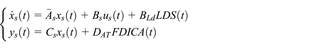
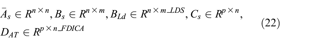
where
It is clear that PAGG is limited. However, the area control error signal is regularly checked, and the automatic generation control has some rules about the behavior of the area control error signal. Therefore, an alarm is raised if an irrational change occurs in the area control error signal (Ameli et al., 2018). Considering this fact, the attacker may attempt to manipulate the area control error signal carefully. As a result, area control error signal is also limited. Here, non-linear sliding mode observer is used for fault detection. Therefore, it is necessary to convert the state-space model into the canonical form. At first, the system output decomposes into two subsystems: subsystem 1 including the system output without FDICA and subsystem 2 including the system output with FDICA. An orthogonal matrix is used to decompose the system output as indicated in equation (23)
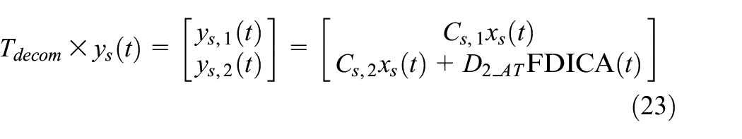
where
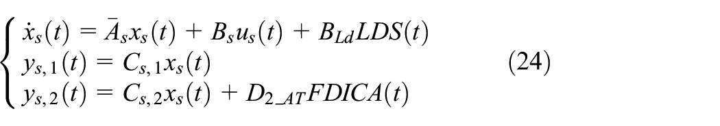
Applying the decomposition matrix, the state-space model of automatic generation control can be rewritten as in equation (24)
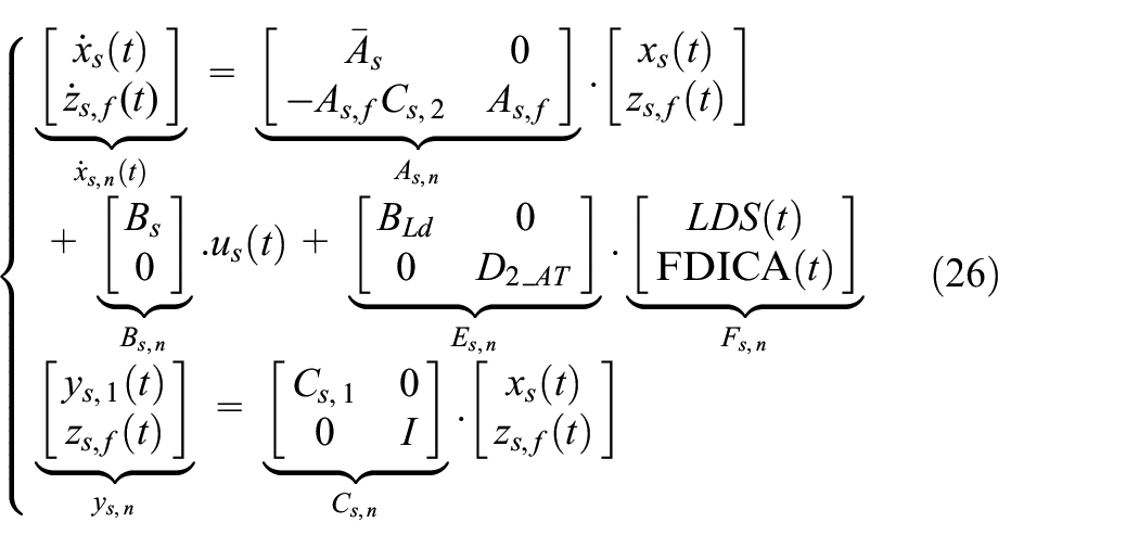
In the next step, the purpose is to displace

where
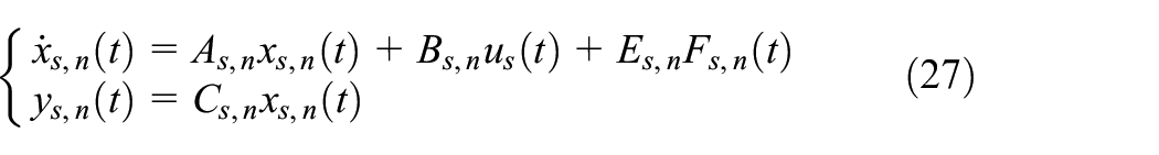
Considering the new variables, the new state-space model of automatic generation control in equation (26) can be written as equation (27)
In the next step, a non-linear sliding mode observer is designed for FDICA reconstruction and calculating PDR. To this purpose, the following conditions must be satisfied (Edwards et al., 2000).
Condition 1: Rank
Condition 2: The invariant zeroes of (
If the above conditions are satisfied, change of coordinate (
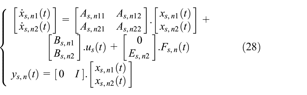
where
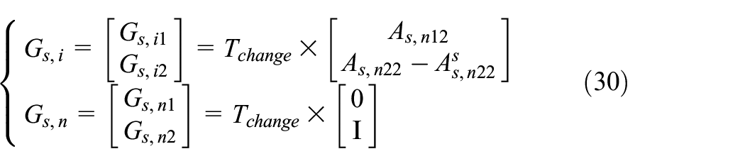
For a system with the mentioned canonical form in equation (28), non-linear sliding mode observer is designed as in equation (29) (Alwi et al., 2011; Edwards et al., 2000; Shtessel et al., 2014)
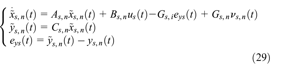
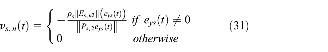
where
where
where
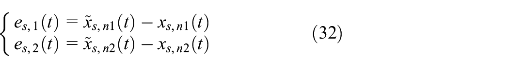
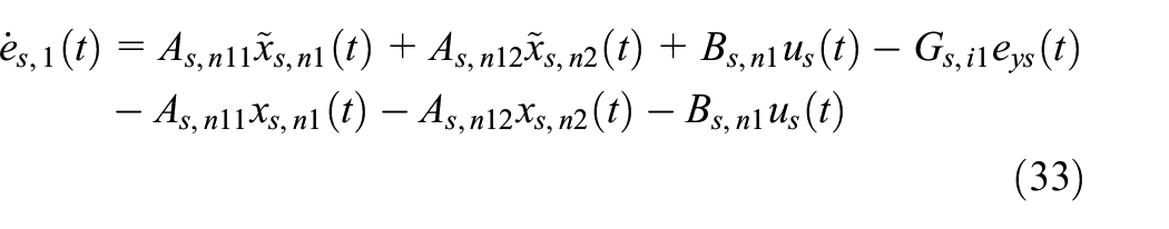
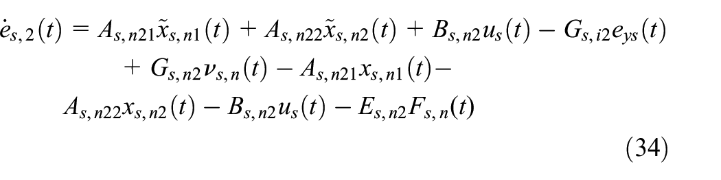
The first derivation of equation (32) with respect to time is given in equations (33) and (34)
According to the idea behind non-linear sliding mode observer, in the sliding motion,
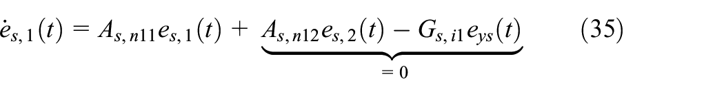
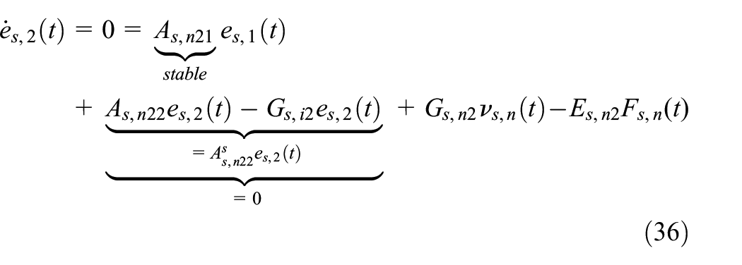
From equation (36) and considering that
By adding
where
Removing FDICA and compensating the ULDS
After FDICA detection, urgent action is required to mitigate the disruptive effect of it. Active disturbance rejection control has an excellent performance to mitigate the adverse effect of faults in the uncertain and noisy environment due to its fast action. Active disturbance rejection control with an extended state observer is used to estimate the disturbance and reject it. Extended state observer cannot separate FDICA from LDS. Therefore, it is better to combine the non-linear sliding mode observer with active disturbance rejection control. In this paper, non-linear sliding mode observer is used instead of extended state observer to separate and reconstruct FDICA and LDS simultaneously, and common active disturbance rejection control will be modified to remove FDICA and control the ULDS. In the following, the design procedure of modified active disturbance rejection control is given.
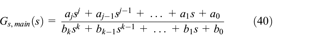
Consider a system with the following definition, as in equation (39)

where
where
where
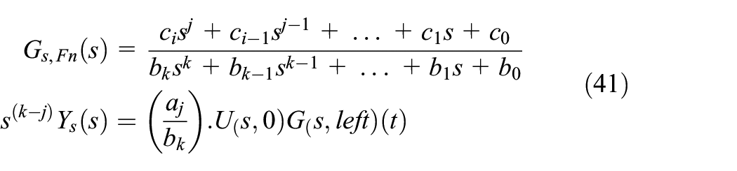
To design active disturbance rejection control, it is enough to transform the system model as in equation (42)
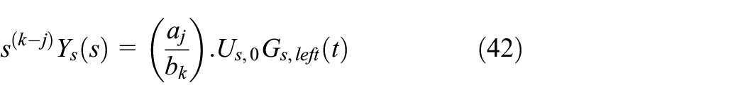
or equivalently transform to the time domain as in equation (43)
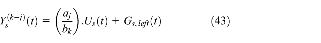
where
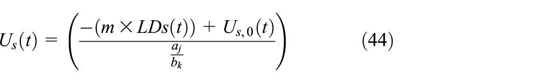
Substituting equation (44) in equation (43), the system model can be written as in equation (45)
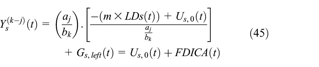
The

With substituting equation (46) in equation (44), the system input is designed as in equation (47)
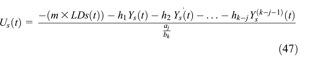
where
The main problem is that

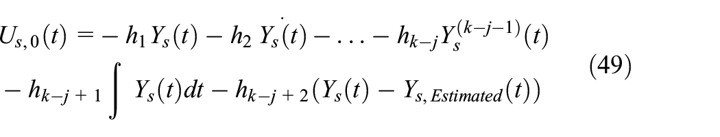
There is always some difference between the estimated and real value. As a third step of modifying the active disturbance rejection control, the control law of active disturbance rejection control will be changed to cover this lacuna. To this end, a feedback from the output and an integrator have been used to reach the final error to zero; therefore, the mentioned control law in equation (46) is changed to equation (49)
The modified active disturbance rejection control is shown in Figure 2.
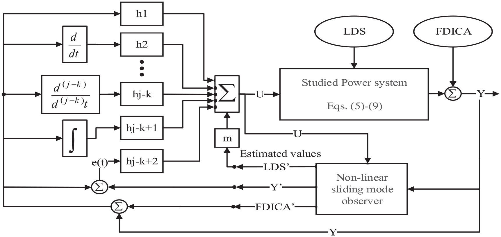
The structure of the modified active disturbance rejection control.
Stability analysis
The stability of the proposed method depends on the stability of non-linear sliding mode observer that estimates the FDICA and the LDS. Inspired from Edwards and Spurgeon (1994) and Zhang et al. (2012), the Lyapunov method is used to investigate the stability of non-linear sliding mode observer. The Lyapunov functions are considered as equation (50)
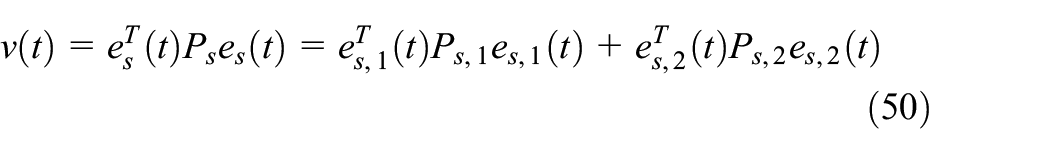
where
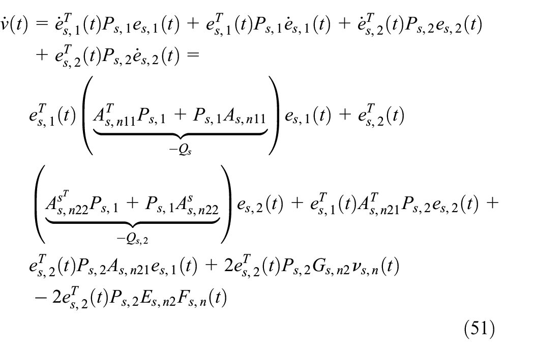
By considering
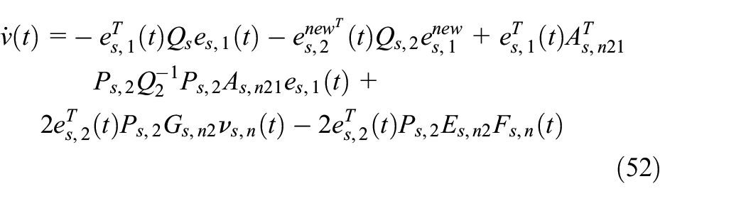
Consider
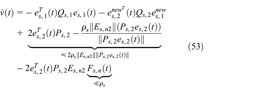
Since, in the automatic generation control, the area control error signal is regularly checked, an alarm is raised if an irrational change occurs; therefore, area control error signal is also limited. As a result,

Therefore
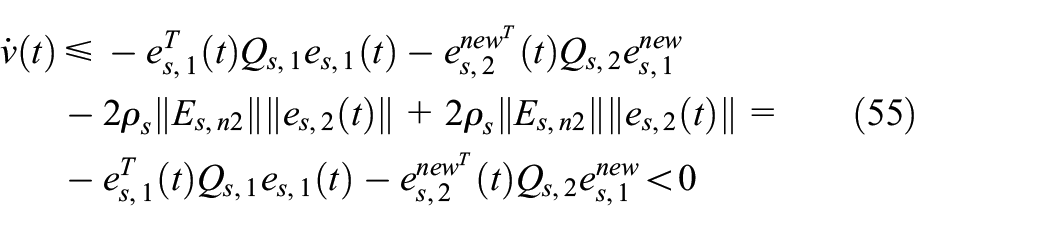
Therefore, the stability of the non-linear sliding mode observer in completely proved. With the stable non-linear sliding mode observer, the estimations will be very close to the actual values.
The proposed algorithm
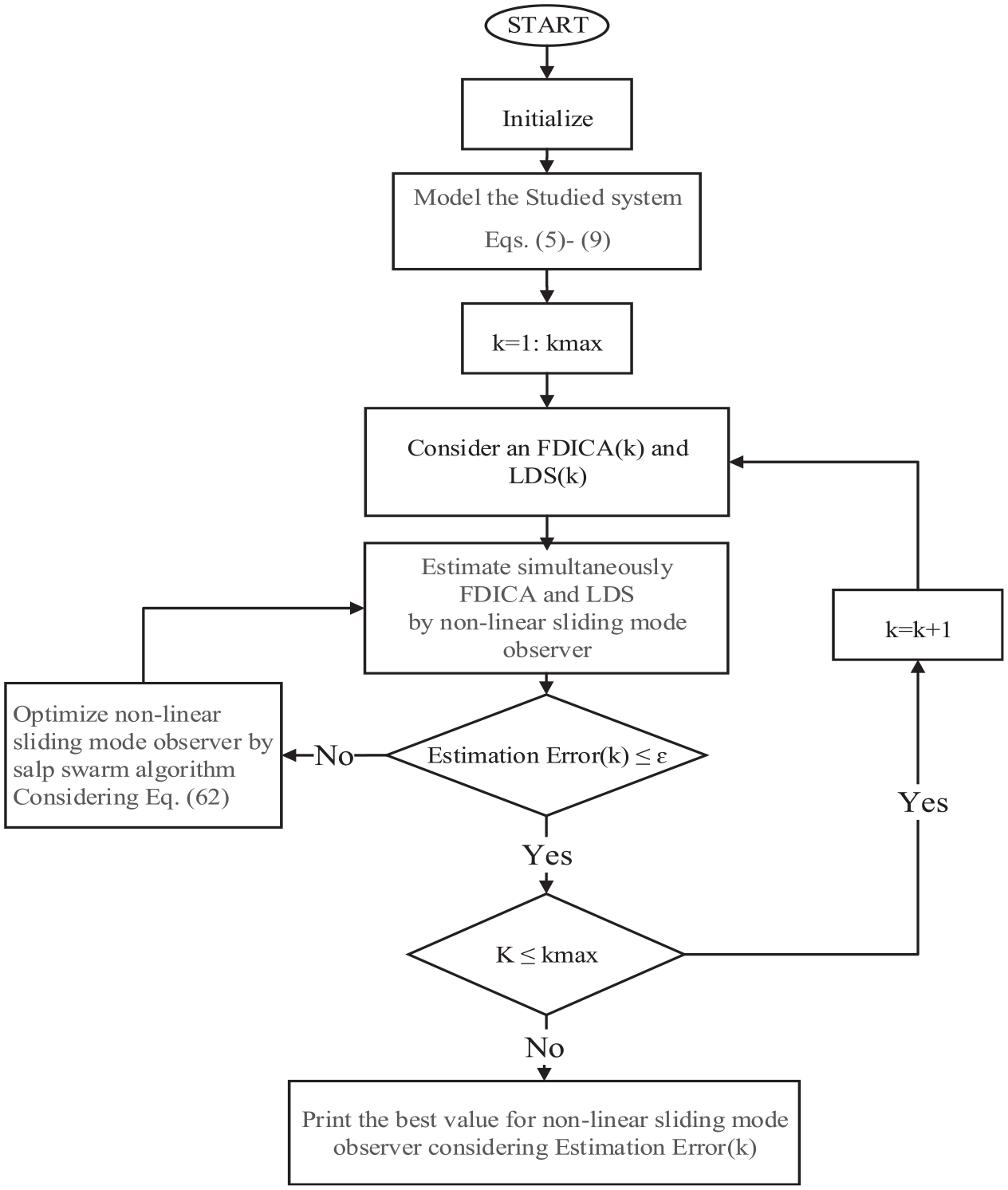
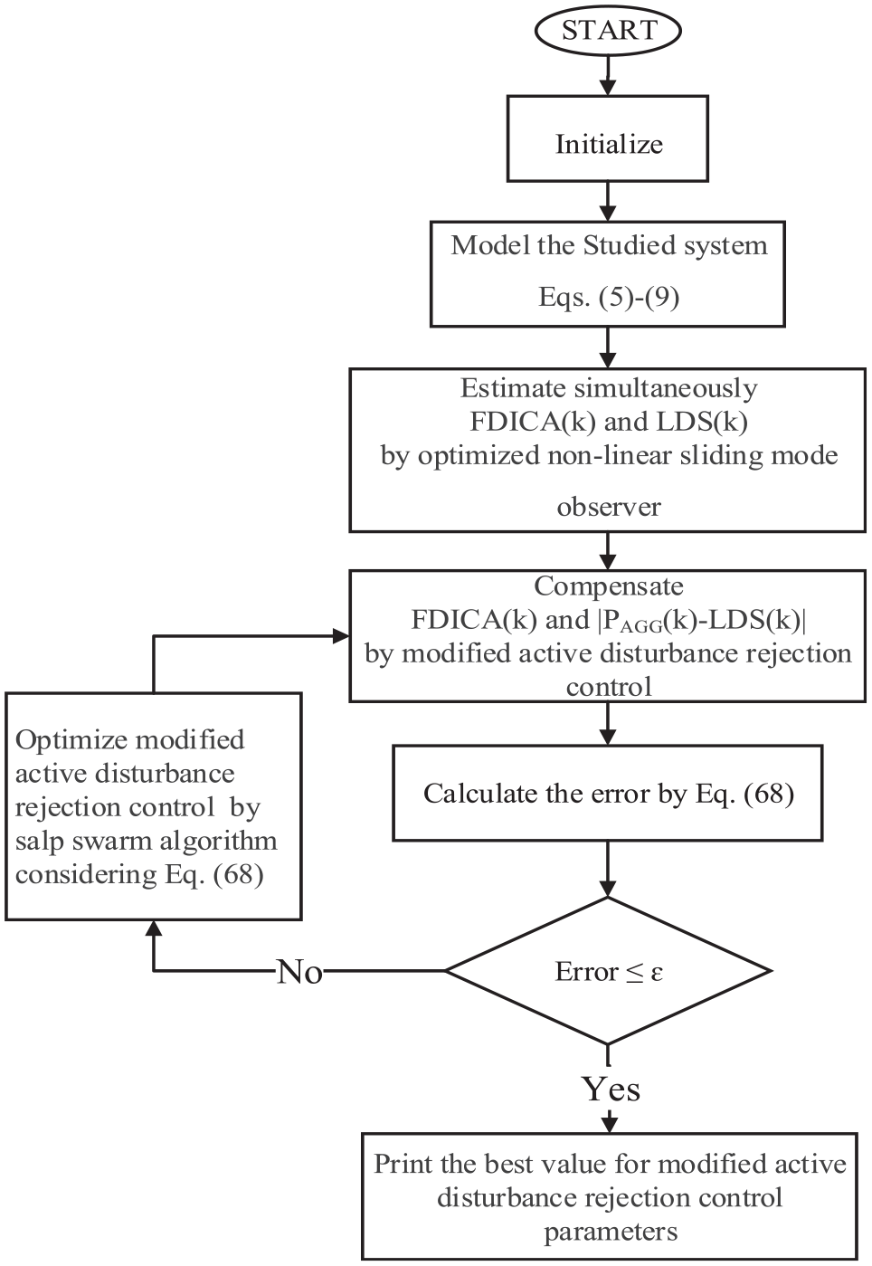
The proposed algorithm is shown in Figure 3 and the procedure of the proposed algorithm is given in the following steps.
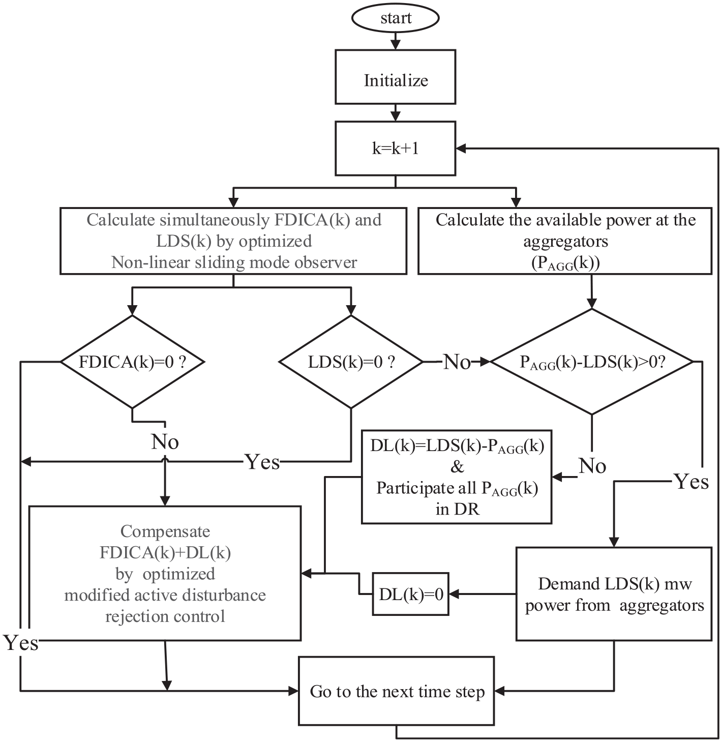
The flowchart of the proposed algorithm.
If PAGG(k) – LDS(k) > 0, the available electrical power at the aggregators can compensate the LDS. However, if PAGG(k) – LDS(k) < 0, the available electrical power at the aggregators cannot compensate the LDS at the time step k.
Results
Definition and decomposition of the studied system under FDICA
To verify the proposed algorithm, it has been tested on a detailed model of the IEEE 9 bus system in the MATLAB software. The studied system is portioned into three controlling areas. The communication time delay for PDR is considered as 0.5 seconds (Babahajiani et al., 2018). To show the robustness of the proposed method, the system parameters are assumed to vary 10% from the nominal value. The single-line diagram of the system under the FDICA condition and participation of demand response is shown in Figure 4.
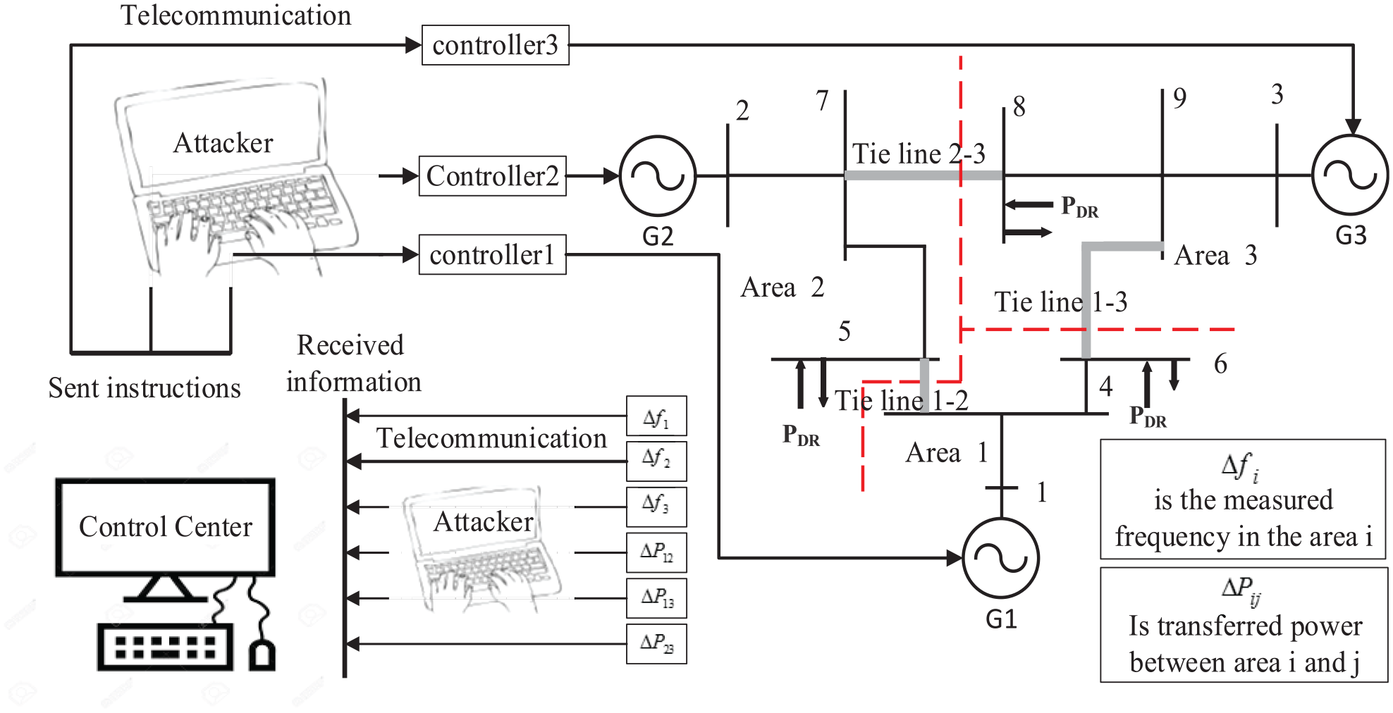
The single-line diagram of the studied system under FDICA.
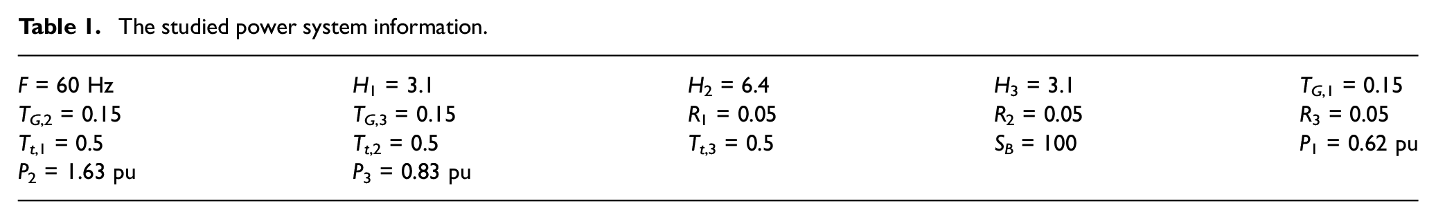
The complete data of the IEEE 9 bus system are given in Yang et al. (2015). In Table 1, the studied power system information is given.
The studied power system information.
As discussed in “Modeling of automatic generation control under FDICA with the presence of demand response program” section, the states in each area are as in equation (56)

There are three areas in the studied system; therefore, the number of states is 12. However, one of the states (
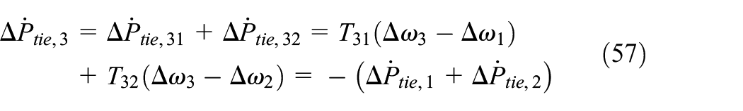
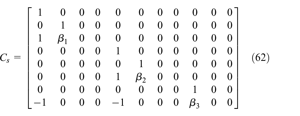
Considering the minimal state-space realization theory, the dependent state is ignored, decreasing the number of states to 11. With respect to this change, the system matrices are designed as indicated in equations (58) to (60)
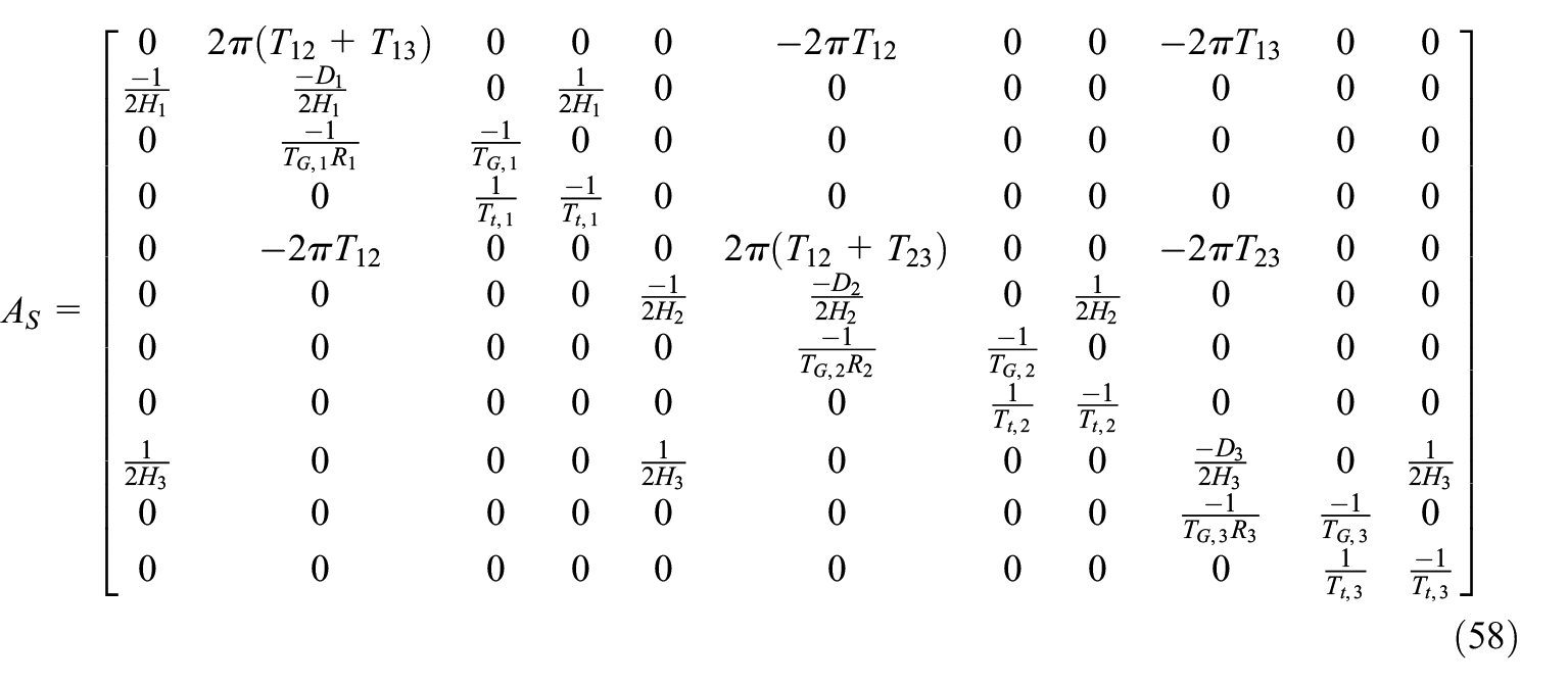
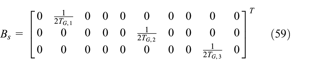
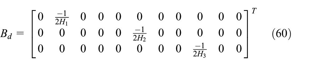
With the elimination of

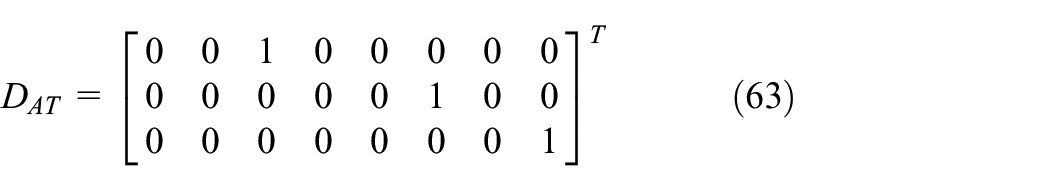
In this paper, it is assumed that the sensors of the system are secured from attack. Therefore, the attacker only can manipulate the transferred information. As a result, only the area control error signal is under attack. The distribution FDICA matrix is defined as in equation (63)
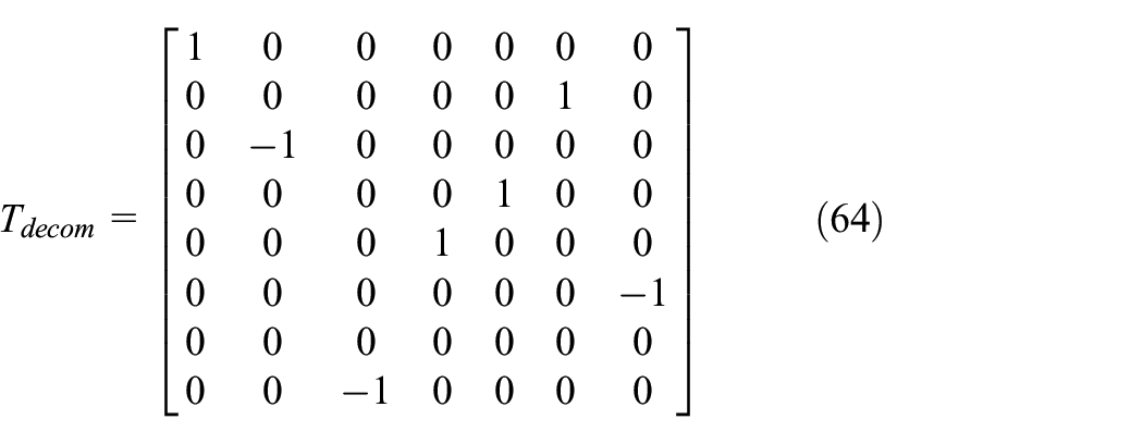
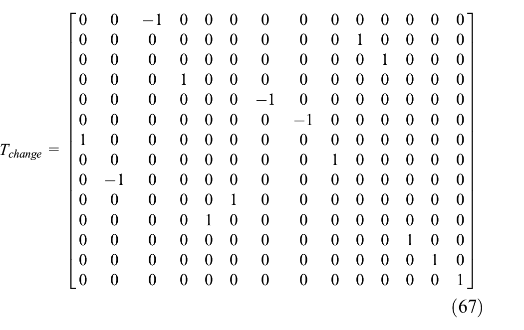
To transform the above system to the canonical form of non-linear sliding mode observer, at first, a decomposition matrix (
Optimization of non-linear sliding mode observer
After decomposition of the system outputs, a filter is needed to displace
The procedure of optimizing the non-linear sliding mode observer is given in Figure 5.
Optimization flowchart of the non-linear sliding mode observer.
The parameters of salp swarm algorithm are given in Table 2.
The parameters of salp swarm algorithm (Mirjalili et al., 2017) .
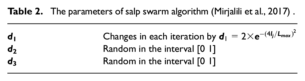
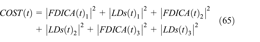
Figure 6 shows the mentioned cost function in equation (65) in the process of optimizing by salp swarm algorithm.
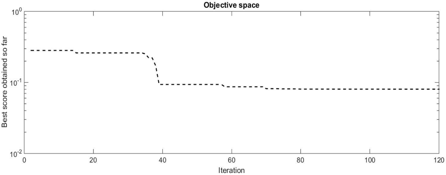
The cost function of salp swarm algorithm for optimizing the non-linear sliding mode observer.
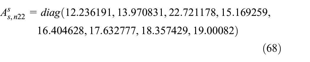
The optimized value for
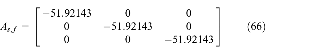
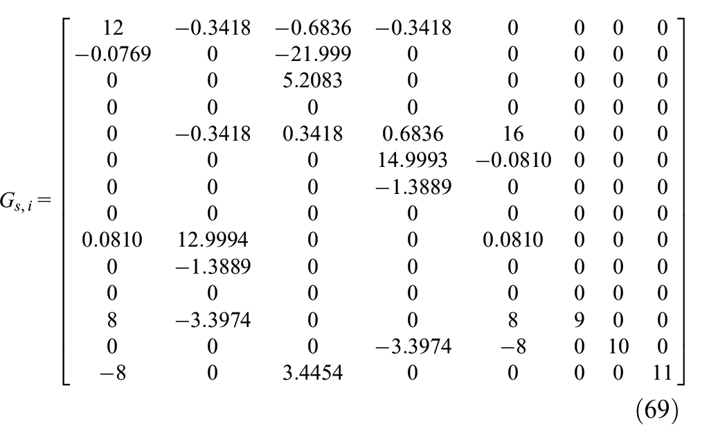
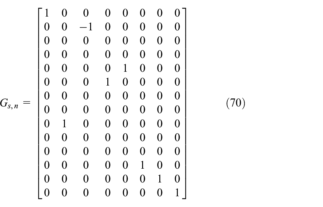
The canonical form of the state equation of the system is obtained by
The stable matrix
The
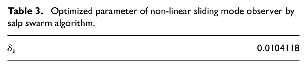
The optimized value for
Optimized parameter of non-linear sliding mode observer by salp swarm algorithm.
Optimization of modified active disturbance rejection control
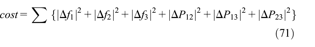
After FDICA detection and reconstruction, the proposed control modified active disturbance rejection control non-linear sliding mode observer is applied to reject the FDICA, and demand response is used to compensate LDS. To this end, the controller gains (Wc1, Wc2, Wc3, Wo1, Wo2, and Wo3) are optimized by salp swarm algorithm. As discussed in the introduction, automatic generation control has two primary responsibilities, including maintaining the frequency in the allowable range and controlling the transferred power between the areas. Therefore, at this time, the cost function is defined by equation (71)
The procedure of optimizing the modified active disturbance rejection control is given in Figure 7.
The procedure of optimizing the modified active disturbance rejection control.
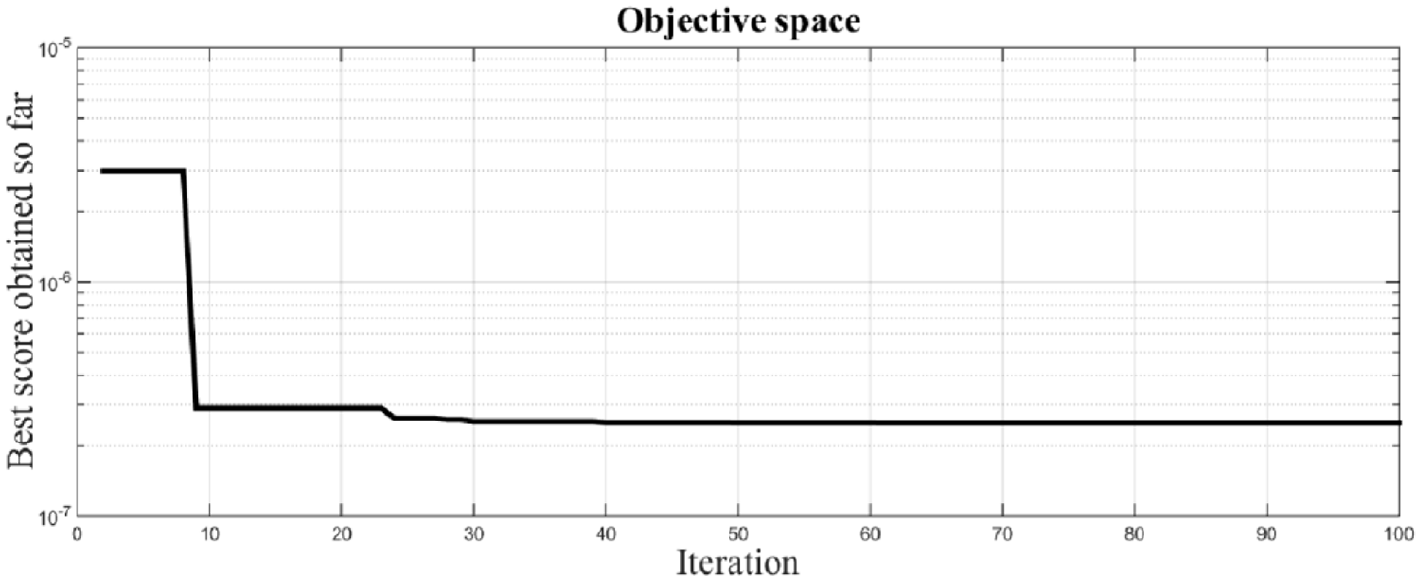
Figure 8 shows the cost function for optimizing the modified active disturbance rejection control.
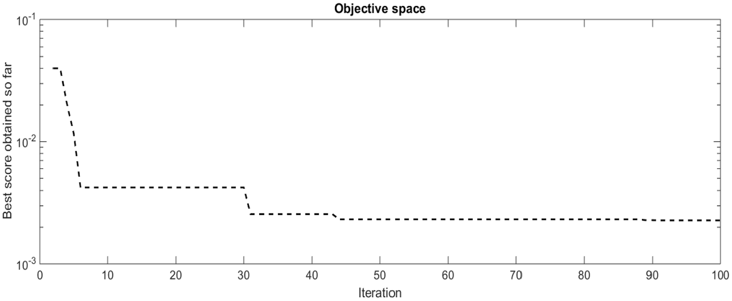
The cost function of salp swarm algorithm for optimizing the modified active disturbance rejection control.
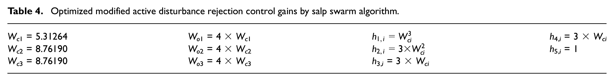
In Table 4, the optimized values of the modified active disturbance rejection control parameters are given.
Optimized modified active disturbance rejection control gains by salp swarm algorithm.
Simulation of different scenarios
Four different scenarios have been simulated to show the effectiveness of the proposed method. To consider the conditions as the worst condition, FDICA is considered periodically random and limited. In scenarios 1 and 2, the focus is on the reconstruction of FDICA and LDS signals. In scenarios 3 and 4, the power system frequency fluctuations are investigated by applying the proposed method.
Scenario 1
In this scenario, LDS occurs in area 1 while an FDICA has happened in area 1. To consider the conditions as a worst condition, FDICA is considered as periodically random in all scenarios, and it is stimulated by white noise. The performance of the non-linear sliding mode observer in reconstructing of FDICA and LDS has been shown in Figure 9.
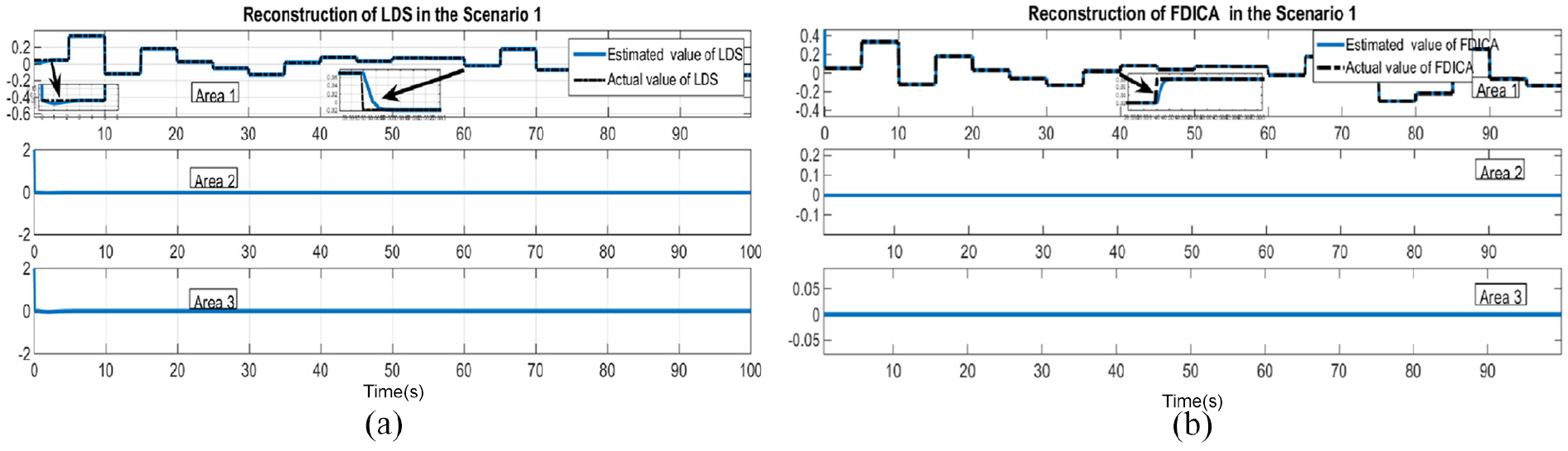
Reconstruction and finding out the location of (a) LDS and (b) FDICA in scenario 1 by non-linear sliding mode observer.
Scenario 2
In scenario 2, LDS occurs in areas 2 and 3 while FDICA has happened in areas 2 and 3. The performance of the non-linear sliding mode observer in reconstructing of FDICA and LDS has been shown in Figure 10.
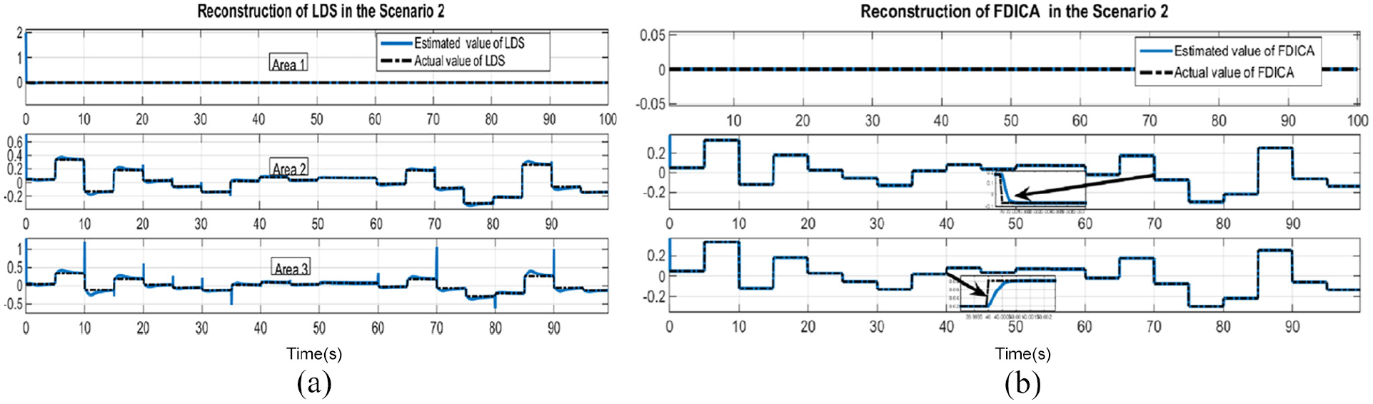
Reconstruction and finding out the location of (a) Reconstruction of LDS in the Scenario 2 (b) FDICA in scenario 2 by non-linear sliding mode observer.
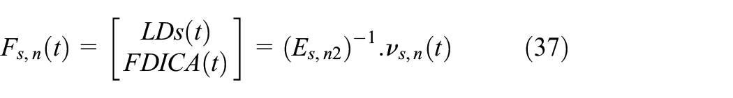
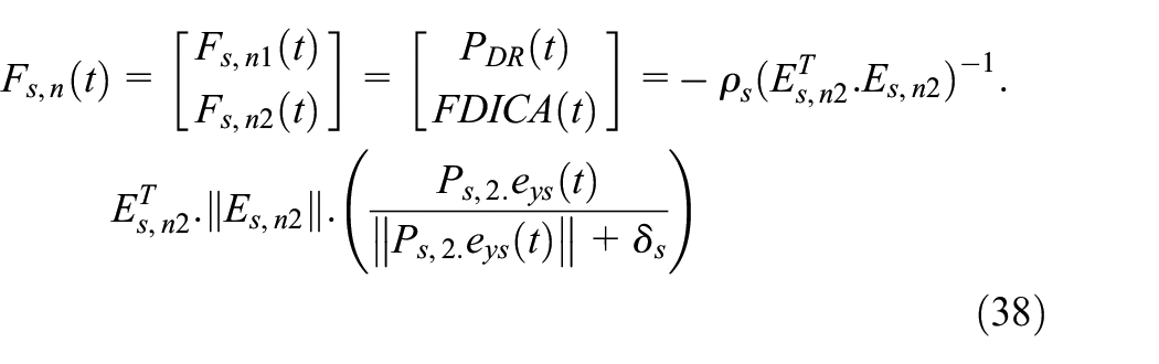
Two mentioned scenarios are simulated in the MATLAB environment to show the effectiveness of the proposed method. According to Figure 9(a), it is clear that the LDS has happened in area 1. In areas 2 and 3, there are not any LDS, and the estimated values for LDS in those areas are zero. Considering Figure 9(b), it is evident that the FDICA has happened in area 1. In areas 2 and 3, the estimated values for FDICA are zero. There is a similar interpretation for Figure 10. As shown, with monitoring equation (38), the location and significance of the FDICA and LDS can be found.
Scenario 3
In this scenario, an LDS occurs in area 1 while an FDICA has happened in that area. It is assumed that the available electrical power in the aggregators cannot compensate for all the LDS and can compensate only 0.8 pu of LDS. Thus, modified active disturbance rejection control—non-linear sliding mode observer—must participate in compensation of 0.2 pu LDS and remove FDICA. The proportional integral derivative (PID) controller as a secondary controller in automatic generation control has been utilized to compare with the proposed method. The parameters of the PID controller are optimized with the salp swarm algorithm considering the cost function in equation (71). The optimized values for the parameters of the PID controller are given in Table 5.
Optimized value for the parameters of the PID controller.
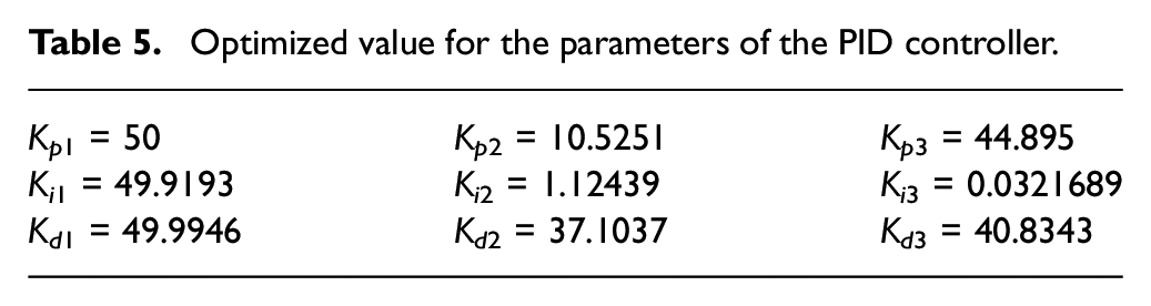
Figure 11 shows the cost function for optimizing the PID controller.
The cost function for optimizing the PID controller.
A comparison between the proposed method and the PID controller in settling the power system frequency fluctuations in scenario 3 is given in Figure 12.
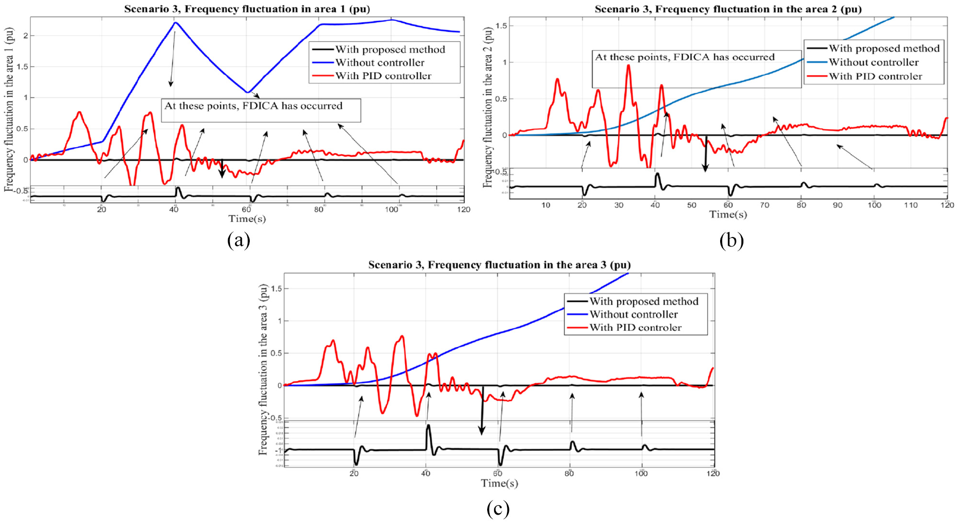
The power system frequency fluctuations in scenario 3 in (a) area 1, (b) area 2, and (c) area 3.
As it is evident, without controller, the power system frequency is increasing or decreasing under the FDICA. Considering Figure 12, the effectiveness of the proposed method in comparison with the non-controlling situation and PID controller is apparent. Attackers by FDICA attempt to disrupt the power system performance, resulting in increasing or decreasing the power system frequency. Also, there are the same results as ULDS. As shown in Figure 12, without applying the preventing action in contrast with FDICA and ULDS, the power system frequency will be increased or decreased. Therefore, to have a reliable power system, it is urgent to do a preventing action in contrast with FDICA and ULDS. Considering Figure 12, the effectiveness of the proposed method in contrast with FDICA and ULDS is apparent.
Scenario 4
In this scenario, LDS occurs in areas 1 and 2 while FDICA has happened in areas 1 and 2. It is assumed that the available electrical power in the aggregators can compensate for the 0.8 pu LDS in area 2 and the whole of LDS in area 1. Figure 13 shows the comparison between the proposed method and PID controller as a secondary controller in automatic generation control in settling the power system frequency fluctuations in scenario 4.
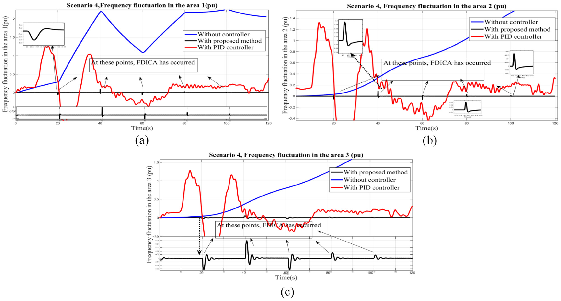
The power system frequency fluctuations in scenario 4 in (a) area 1, (b) area 2, and (c) area 3.
Scenario 4 was simulated to emphasize the effectiveness of the proposed method for worst condition. Considering Figure 13, it is evident that the power system frequency is settled in the permissible range, even with FDICA and participation of the demand response program. As shown, after occurring FDICA in less than 5 seconds, the frequency fluctuations tend to almost zero.
Conclusion
This paper presented a new method for simultaneous cyber-attack tolerant and participation of demand response program in the load frequency control. In the proposed method, the most important step is simultaneous accurate estimation of FDICA and LDS by non-linear sliding mode observer. The stability analysis by the Lyapunov method emphasizes the ability of the proposed method for stable and accurate estimation. After estimation step, part of the LDS compensates by the demand response program considering the available power at the aggregators. Then, an active disturbance rejection control is modified to remove FDICA and control the ULDS. Finally, an algorithm is presented based on the estimations of non-linear sliding mode observer and the ability of proposed modified active disturbance rejection control to remove the FDICA and control the ULDS. The presented algorithm controls the power system frequency under FDICA, LDS conditions, and the demand response program; as a result, after occurring FDICA in less than 5 seconds, the frequency fluctuations tend to almost zero. The presented conditions in designing the non-linear sliding mode observer and decomposition of the studied system into two subsystems are the limitations of the proposed method. The results of the several simulation scenarios and comparison with an optimized PID controller as a secondary controller in automatic generation control indicate the efficient performance of the proposed method in the detection and reconstruction of FDICA and LDS as well as controlling power system frequency under FDICA, LDS conditions, and demand response program.
Footnotes
Appendix A
Author contributions
S.H.R. contributed to conceptualization, methodology, software, investigation, and writing original draft. H.M. contributed to software, validation, supervision, writing-reviewing, and editing. A.B. contributed to validation, supervision, reviewing, and editing.
Declaration of conflicting interests
The author(s) declared no potential conflicts of interest with respect to the research, authorship, and/or publication of this article.
Funding
The author(s) received no financial support for the research, authorship, and/or publication of this article.