
Abstract
With the continuous development of pipeline transportation industry, pipeline leakage often occurs, posing a great threat to people’s lives and property safety. In order to improve the detection accuracy of natural gas pipeline leakage, a pipeline leakage detection method based on improved variational mode decomposition algorithm and Lempel–Ziv complexity analysis is proposed. In this work, the normalized mutual information is used to determine the decomposition level K of variational mode decomposition, and the Lempel–Ziv complexity analysis algorithm is used to extract pipeline signal feature. The results show that the proposed leakage detection method has higher classification accuracy than other methods, which verifies the effectiveness of this method in the process of pipeline leakage detection.
Keywords
Introduction
With the increasing demand for oil and gas and the vigorous development of pipeline transportation industry, more and more long-distance pipelines are gradually being put into use (Liu et al., 2019a). However, leakage occurs from time to time (Wang et al., 2019b), resulting in resources waste, environmental pollution, and even serious threat to people’s lives (Wang et al., 2017). In order to avoid frequent leakage accidents, the methods commonly used in pipeline leakage detection include dynamic pressure wave method (Liu et al., 2017), acoustic method (Yu et al., 2016), model-based detection method (Rui et al., 2017), and leakage detection method based on wireless sensor network (Okpare et al., 2018) and so on. Among them, the acoustic detection method can meet the requirements of wide frequency response range, high sensitivity, low false alarm rate, and good real-time detection, so it has been widely used (Quy et al., 2019; Wang et al., 2016c).
Because the sensor is interfered by the noise generated by the pipeline leak detection system itself and the complex environment, it directly affects the application effect of the acoustic wave detection method (Xiao et al., 2016). Therefore, in order to improve the accuracy of leakage detection (Xiao et al., 2017), the pipeline signal must be pre-processed for noise reduction. In 2014, Dragomiretskiy and Zosso (2014) proposed the variational mode decomposition (VMD) algorithm. It has a good processing effect on nonlinear and non-stationary signals, and can adaptively decompose the signal into a series of intrinsic mode functions (IMFs). Hausdorff distance was used to distinguish the effective and non-effective components of image after two-dimensional VMD (Gao et al., 2020), then used wavelet denoising to process non-effective modes, so as to achieve the purpose of pipeline image denoising. Although VMD has the advantages of high accuracy and strong noise robustness in signal decomposition, it has the disadvantage that the number of decomposition layer K needs to be determined in advance and it will directly affect the decomposition effect of VMD on the signal (Wang et al., 2019a). In order to determine the K of VMD, many scholars have carried out in-depth research (Li et al., 2020). Particle swarm optimization algorithm (PSO) was used to optimize the parameters of VMD (Wang et al., 2020), and applied it to detect the pipeline leakage signal. However, this method has the disadvantage of long time-consuming in parameter optimization process. Lu et al. (2020b) used the empirical mode decomposition (EMD) method to select K value, and combined VMD with the improved Bhattacharyya distance to denoise the leakage signal of natural gas pipeline, but due to the problem of mode aliasing in EMD algorithm, VMD will appear over-decomposition phenomenon. So, it is necessary to design an efficient and accurate K value determination method.
In addition, in the process of acoustic leakage detection, feature extraction is also very important to improve the accuracy of detection (Jin et al., 2014). Therefore, how to extract leakage characteristics from the signal has a great influence on reducing the false alarm rate of leakage detection. VMD was combined with variance contribution rate to denoise the pipeline signal, and extracted feature parameters, such as standard deviation, absolute mean, and information entropy, then input them to support vector machine (SVM) for classification, with the detection accuracy of 98.33% (Zhou et al., 2020). Markov feature and statistical features were extracted to detect the leakage of crude oil pipeline, and the results showed that the final accuracy can reach 99.17% (Liu et al., 2019a). Wavelet transform was used to preprocess the natural gas pipeline signal, and the features were selected through Relief-F algorithm, and then combined with SVM to identify the leakage. The accuracy was 99.4%, indicating that this method is an effective pipeline leakage detection method (Xiao et al., 2019). Although the above methods have achieved good detection results, there are also a small amount of detection errors, so the extraction of a more effective feature that is beneficial to leakage identification needs further study. For non-stationary signals, the Lempel–Ziv index was calculated to characterize the rate of generating new patterns when the signals changed, then measured the complexity of time series (Tang et al., 2019). The results showed that the Lempel–Ziv index can quantitatively measure the complexity of nonlinear signals and effectively distinguish different signals. Therefore, the Lempel–Ziv complexity analysis algorithm was used in this paper to extract the feature of pipeline signals.
For the method of determining the VMD parameter K value by EMD, here are obvious limitations of this method because the EMD algorithm has the problem of mode mixing, which can directly lead to the over-decomposition of VMD. Using intelligent optimization algorithm to select VMD parameter value will consume a lot of time and seriously reduce the use efficiency of VMD. In addition, the traditional time–frequency domain features are non-stationary, resulting in poor leakage identification. To improve the pipeline leakage recognition rate, the main contribution of this paper is to propose an improved VMD algorithm that solves the problem of K value selection and improves the leakage detection accuracy by extracting the Lempel–Ziv complexity feature (LZC). First, the preliminary K value is obtained by EMD decomposition, and the K value is continuously updated by the normalized mutual information between the original signal and each IMF until the final VMD decomposition layer K value is obtained. Next, the effective modes after VMD decomposition are selected using dispersion entropy and reconstructed to denoise the pipeline signal. Finally, the Lempel–Ziv complexity analysis algorithm is used to analyze the denoised pipeline signal to extract the Lempel–Ziv complexity feature, and the effectiveness of the proposed feature for leakage detection is verified by SVM classifier.
The rest of this paper is organized as follows. Section “Theory” introduces the principle of VMD and Lempel–Ziv complexity analysis algorithm. Section “Proposed method” presents the method of determining the K value, the VMD-based denoising method, and the Lempel–Ziv complexity feature extraction method. Section “Experimental processing results and discussion” introduces the experimental device and data, and uses the proposed method to detect the pipeline leakage. Finally, section “Conclusion” draws a conclusion.
Theory
VMD
As a new adaptive decomposition algorithm, VMD can decompose signals into multimodal components with different center frequencies (Dragomiretskiy and Zosso, 2014). The original signal
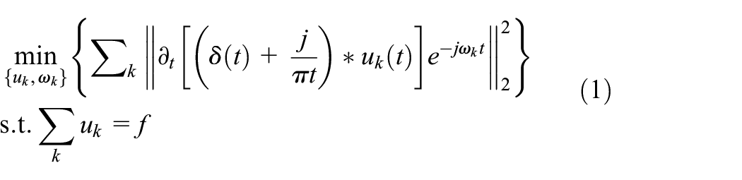
where
The optimal solution of constraint variational model is obtained based on the introduction of quadratic penalty factor
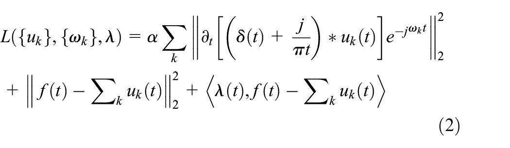
Using the alternating direction method of multipliers (ADMM) to solve the above variational model, K IMFs are finally obtained. The specific operation of VMD is shown in Algorithm 1.

From the VMD decomposition process, it is known that the K value is crucial to the decomposition effect of VMD. And according to the analysis in references (Yang et al., 2017), the setting of the mode number K directly determines the performance of VMD decomposition, and the selection of K value by human experience often leads to the over-decomposition or under-decomposition. Therefore, the K value is chosen to be studied in this paper. For the two key parameters of VMD, decomposition layer K and penalty factor α: the value of α is set to 2000 according to Lu et al. (2020b), and the value of K is discussed and analyzed in this study.
Lempel–Ziv complexity analysis
Lempel and Ziv put forward an algorithm for measuring the complexity of a finite length signal, Lempel–Ziv complexity analysis, which can characterize the rate of generating new patterns when the signal changes (Ziv and Lempel, 1977). Algorithm 2 shows the procedure for calculating the Lempel–Ziv complexity of the signal sequence
Step 1: Coarse graining of numerical sequences.
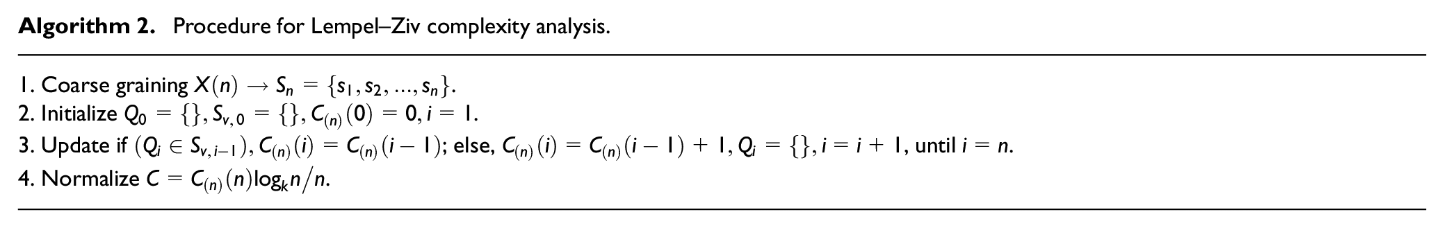
Step 2: Parameter initialization.
Sequences
Step 3: Calculate the Lempel–Ziv complexity value of the sequence.
Let
Step 4: Normalized Lempel–Ziv complexity value.
For the convenience of data analysis, the normalized reference formula is used to calculate the complexity of the signal sequence. The value of

where, since
Proposed Method
Improved VMD based on EMD and normalized mutual information
For determining the VMD decomposition layer number K, the improved VMD method shown in Figure 1 is proposed in this section, and the specific steps are as follows:
Step 1: EMD is applied to decompose the signal
Step 2: The mode number K obtained from EMD decomposition is initially set as the decomposition layer K of VMD.
Step 3: Use VMD to decompose
Step 4: Calculate the normalized mutual information (MI) between IMF and
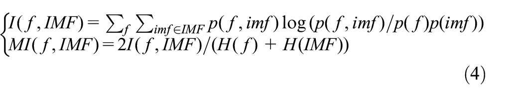
where
Step 5: After a large number of experiments, the threshold value of ΔMI (the difference between adjacent MIs) is determined as 0.001. Compare the ΔMI(i), if equation (5) holds, it means that two modes of frequency aliasing are generated. There is over-decomposition phenomenon in VMD decomposition, reset K = K – 1, and repeat Step 3, Step 4 until equation (5) does not hold, then the loop ends, and the optimal K of VMD decomposition is obtained. On the contrary, if equation (5) does not hold at the beginning, then there is no need to carry out the loop step, and the mode number K obtained by EMD decomposition is the final decomposition layer K of VMD. In addition, the mode number of EMD decomposition is taken as the maximum upper limit of the layer number K of VMD decomposition, since the K value is set from large to small, so the situation of under-decomposition of VMD is avoided to some extent

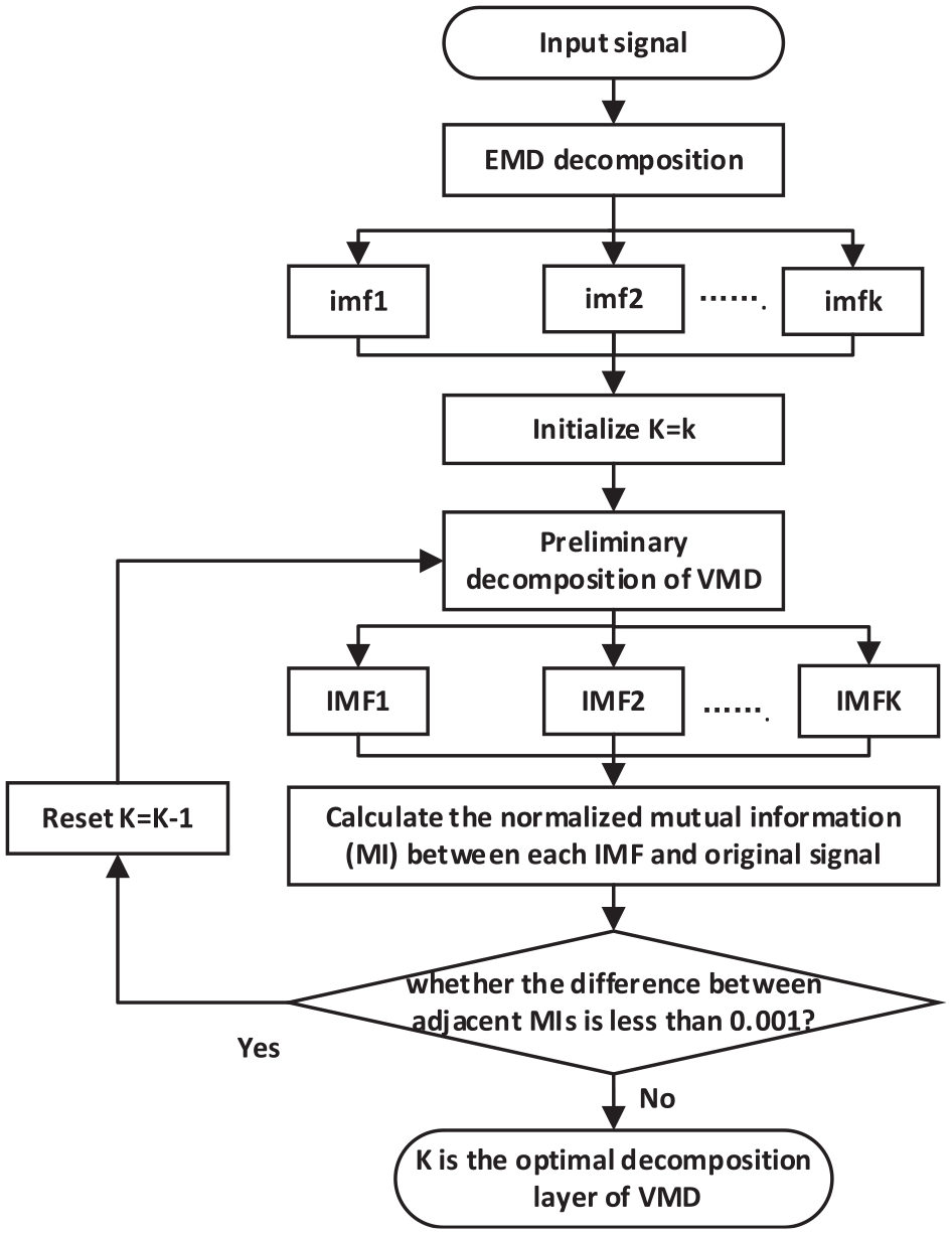
Flowchart of the improved VMD.
The proposed pipeline leakage detection method
To ensure good classification performance, the noise reduction preprocessing should be carried out for the pipeline signal first and then use the Lempel–Ziv complexity algorithm to analyze the complexity of the denoised signal. Based on the improved VMD, dispersion entropy, Lempel–Ziv complexity analysis, and SVM, a novel pipeline leakage detection method is proposed as follows:
Step 1: Use the improved VMD proposed in section “Improved VMD based on EMD and normalized mutual information” to decompose pipeline signal and obtain K IMFs.
Step 2: Calculate the dispersion entropy of each IMF, select the IMFs with significantly smaller values as the effective IMFs, and the other IMFs are considered as noisy IMFs.
Step 3: Reconstruct the effective IMFs to get the denoising signal.
Step 4: Binarize the denoised signal, and change the signal into a binary sequence of 0 and 1.
Step 5: Initialize the parameters and iteratively loop to find the Lempel–Ziv complexity value of the sequence.
Step 6: The normalized Lempel–Ziv complexity value is regarded as the final complexity value of the pipeline signal.
Step 7: Take the Lempel–Ziv complexity value as the feature vector and input it to the SVM classifier for training and classification. Figure 2 shows the overall process of pipeline leakage detection method.
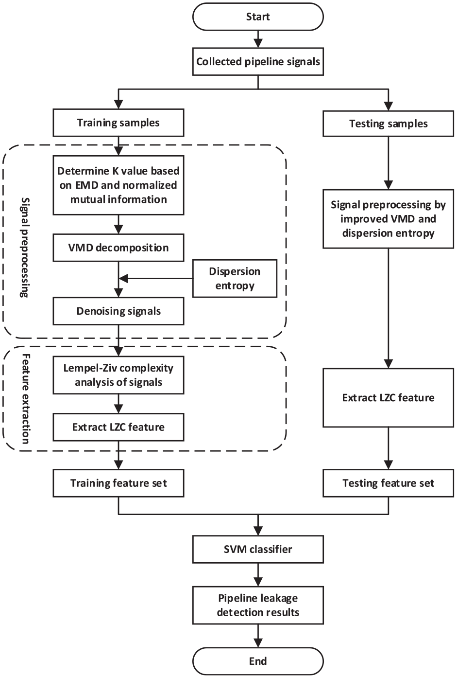
Flowchart of pipeline leakage detection method.
Experimental processing results and discussion
Data source
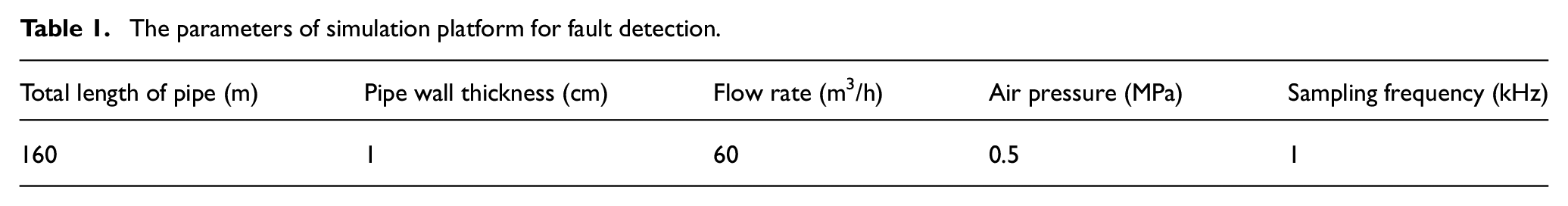
The experimental data in this paper were collected from the natural gas pipeline leakage detection simulation platform. The platform parameters are shown in Table 1, and Figure 3 shows the HD-II pipeline leakage detection system and experimental pipeline diagram. The total length of the pipeline is 160 m, the pipe diameter is DN50, and the wall thickness is 1 cm. Fifteen leakage points are installed in the pipeline, one leakage point every 10 m, and each leakage point is linked with the quarter ball valve to simulate the leakage of the natural gas pipeline in the field. The pipeline fluid is air and powered by the air compressor. The pressure range in the pipeline is 0.1–0.5 MPa, and the flow rate is 60 m3/h.
The parameters of simulation platform for fault detection.
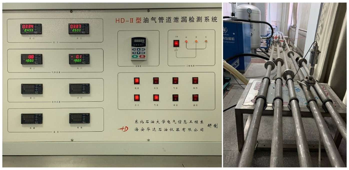
Natural gas pipeline leakage detection platform.
The experiment software adopted the LabVIEW programming environment, through the National Instruments NI-9215 acquisition board card for data acquisition, and the sampling frequency was 1 kHz. When collecting data, the piezoelectric acoustic sensor was used to turn the signal in the pipeline into an electrical signal, and then through the data acquisition board card for signal sampling and transmitted to the computer (the experimental process through compressed air to simulate the natural gas pipeline, and the influencing factors such as medium and pipeline material were not considered temporarily).
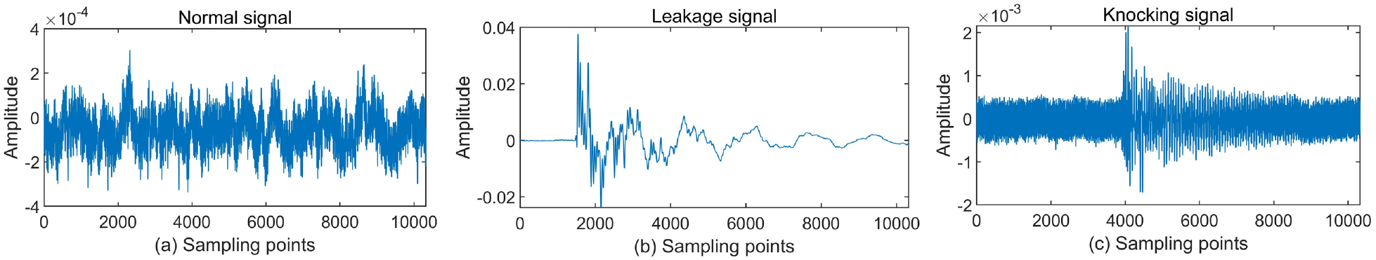
The pipeline signals used in this study were collected at 0.3 MPa pressure, including the following three categories: normal signals, leakage signals, and knocking signals, among which, normal signal was the signal collected when the pipeline natural gas was transported normally, knocking signal was an interference signal simulated by knocking the pipeline, and leakage signal was obtained by quickly switching the quarter ball valve. The time-domain waveforms of the three pipeline signals collected by the experimental platform are shown in Figure 4, and the number of sampling points for each signal is 10,324.
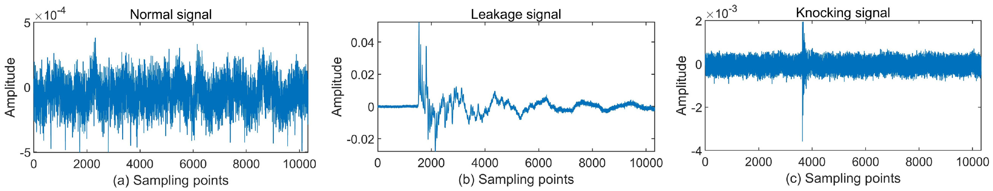
Three time-domain waveforms of sample signals.
From the above figures, three time-domain waveforms contain obvious noise signal, which is not conducive to the feature extraction and leakage detection of the pipeline signal. Therefore, the next main work is to first denoise the signal, highlight the signal feature, and then extract the feature to distinguish three working condition signals and finally carry out classification and identification.
Determination method of K value based on EMD and MI
Before the VMD decomposition of pipeline signal, the decomposition layer K value of VMD must be set first. For the leakage signal, the EMD algorithm was used to decompose it adaptively, as shown in Figure 5, and 10 IMFs was obtained. Next, formula (4) is used to calculate MIs between IMF component and leakage signal to obtain the results of Table 2. From the table, ΔMI between IMF6 and IMF7 is 0.0001 (marked in bold) and less than 0.001, which is considered as over-decomposition. Therefore, according to the method of determining K value in section “Proposed method,” reset K = K – 1, that is, decomposed leakage signal into nine IMFs. MIs of IMFs and leakage signal are calculated again and compared ΔMI between adjacent IMFs, and they are shown in Table 3. It can be observed from the table that ΔMI between IMF3 and IMF4 is 0.0004 (marked in bold), which is less than 0.001. Similarly, over-decomposition has occurred again. Therefore, it is necessary to reset the value of K, let K = 8, repeated the above operations, shown in Table 4. From Table 4, the ΔMIs between all adjacent IMFs are greater than 0.001, indicating that there is no over-decomposition phenomenon in this decomposition. So, the VMD decomposition layer K of leakage signal was finally determined to be 8.
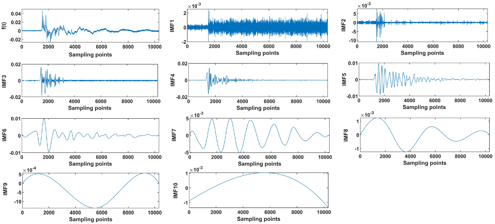
IMFs of leakage signal after EMD decomposition.
MIs value of IMFs and ΔMI(i) between adjacent IMFs (leakage signal, when K = 10).
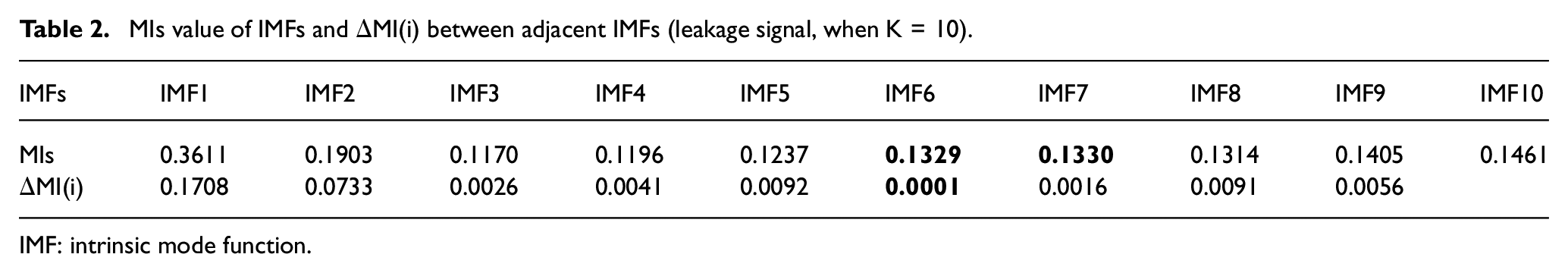
IMF: intrinsic mode function.
MIs value of IMFs and ΔMI(i) between adjacent IMFs (leakage signal, when K = 9).
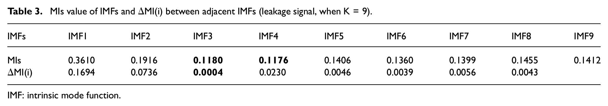
IMF: intrinsic mode function.
MIs value of IMFs and ΔMI(i) between adjacent IMFs (leakage signal. when K = 8).
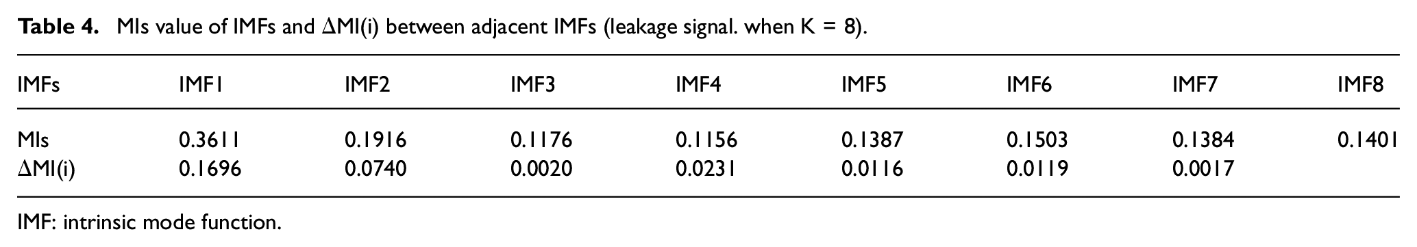
IMF: intrinsic mode function.
The validity of a newly proposed method needs to be verified by repeated experiments. This study then briefly describes the application of the improved VMD method in processing knock signal and normal signal.
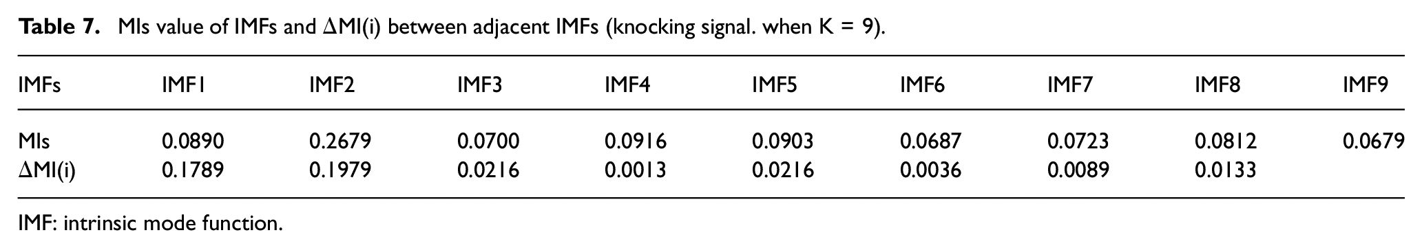
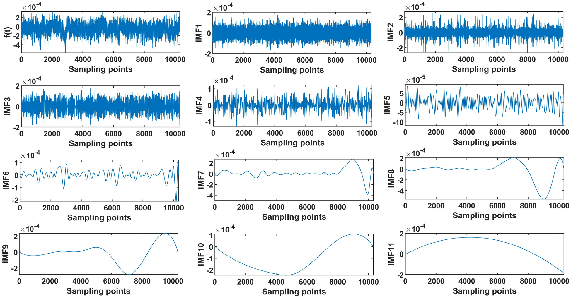
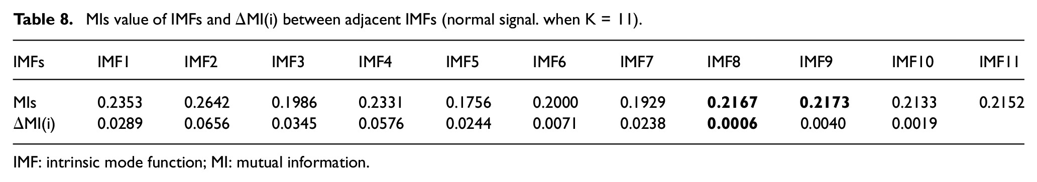
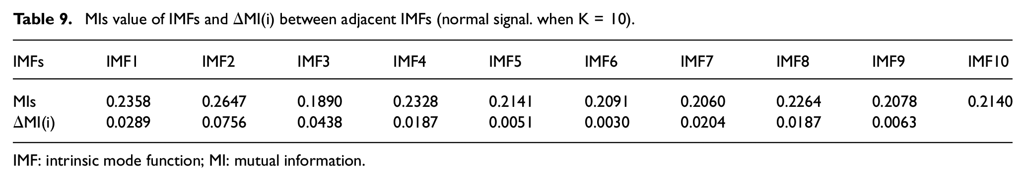
Figure 6 shows EMD decomposition diagram of knocking signal, and Tables 5–7 show the determination process of K value for knocking signal. Figure 7 shows the EMD decomposition diagram of normal signal, and Tables 8 and 9 show the determination process of K value for normal signal. The K values of VMD for knocking signal and normal signal are 9 and 10, respectively. The effective modes are selected and reconstructed using the dispersion entropy. Compared with the noisy pipeline signal shown in Figure 4, the three signals shown in Figure 8 have significant denoising effects.
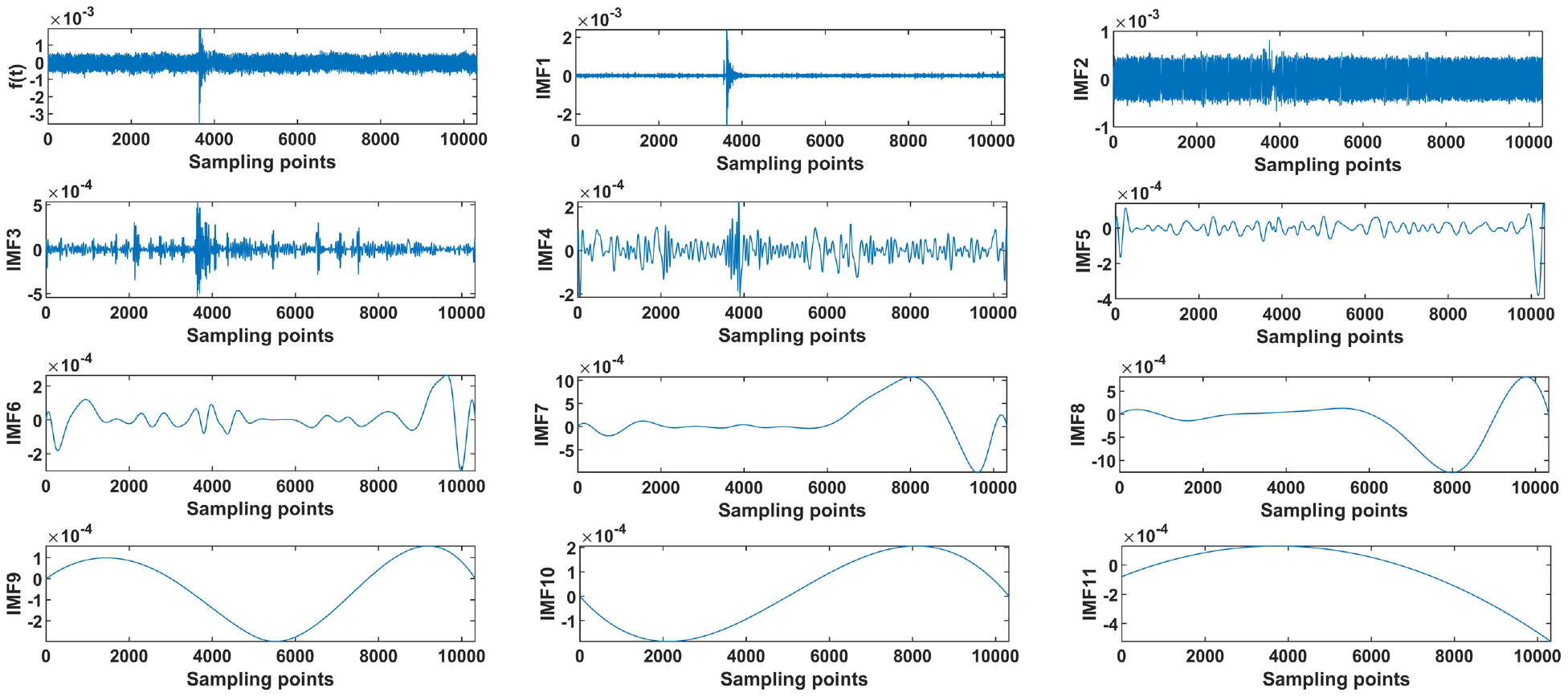
The modes of the knocking signal decomposed by EMD.
MIs value of IMFs and ΔMI(i) between adjacent IMFs (knocking signal. when K = 11).
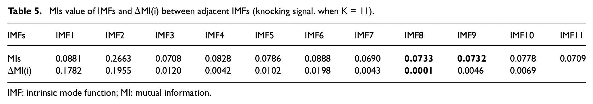
IMF: intrinsic mode function; MI: mutual information.
MIs value of IMFs and ΔMI(i) between adjacent IMFs (knocking signal. when K = 10).
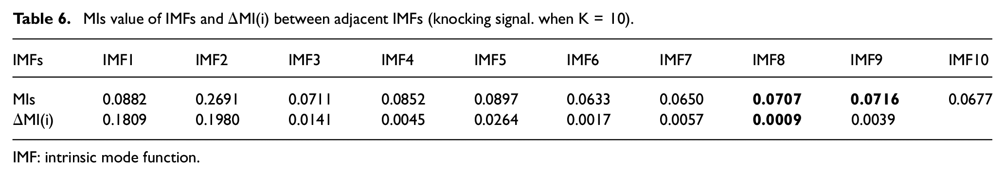
IMF: intrinsic mode function.
MIs value of IMFs and ΔMI(i) between adjacent IMFs (knocking signal. when K = 9).
IMF: intrinsic mode function.
The modes of the normal signal decomposed by EMD.
MIs value of IMFs and ΔMI(i) between adjacent IMFs (normal signal. when K = 11).
IMF: intrinsic mode function; MI: mutual information.
MIs value of IMFs and ΔMI(i) between adjacent IMFs (normal signal. when K = 10).
IMF: intrinsic mode function; MI: mutual information.
Denoised pipeline signals l of normal, leakage and knocking signal.
Lempel–Ziv complexity feature extraction of pipeline signal
As can be seen intuitively from Figure 4, three kinds of signals—normal, leakage, and knocking signal—have obviously different time-domain characteristics. The normal signal waveform of the pipeline is stable and disordered, without obvious shock or oscillating components. The leakage characteristics of the leakage signal are mainly manifested in the low frequency, and there are obvious leakage components at the moment when the valve is opened to simulate the leakage state. Over time, the magnitude of leakage signal decreases little by little and finally tends to be stable. The knocking signal appears obvious pulse component at the time of striking the pipe, then the signal is accompanied by a period of oscillation, and the signal waveform shows fluctuation.
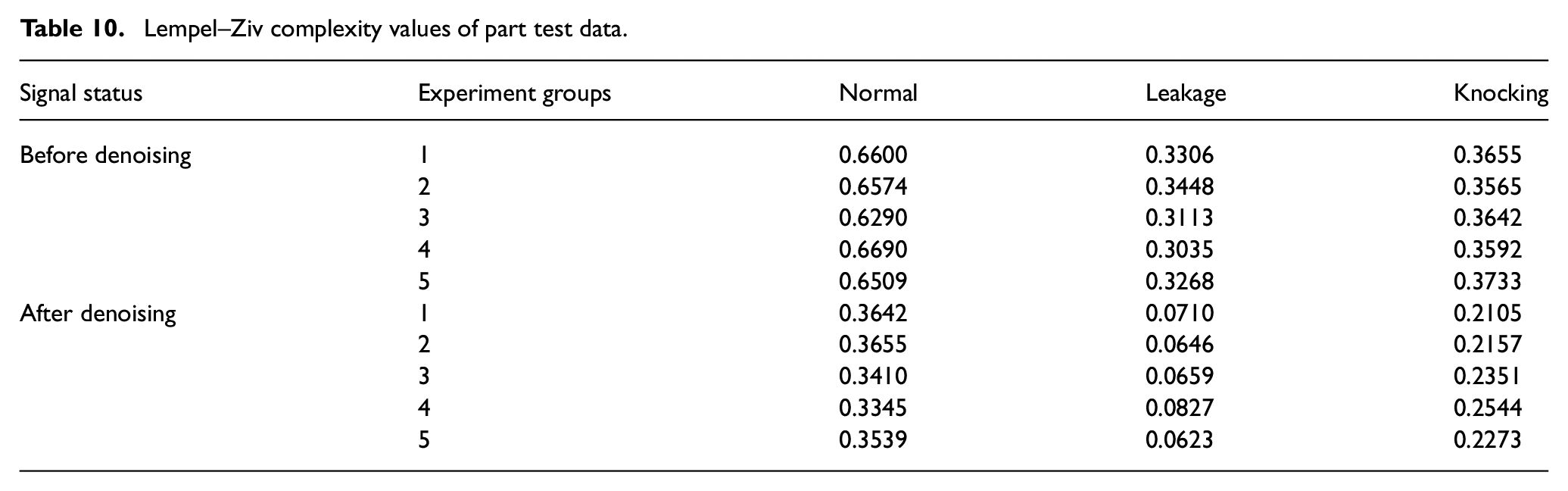
It can be seen from the above analysis that the signals of different pipeline working conditions have different waveforms and show different degrees of complexity. Therefore, for improving the accuracy of pipeline leakage detection, this paper proposed a feature extraction method combining improved VMD and Lempel–Ziv complexity feature for pipeline signal. First, the noise reduction preprocessing was performed on the pipeline signal and then the complexity analysis was carried out for the denoised signal to extract Lempel–Ziv complexity feature. Table 10 shows the Lempel–Ziv complexity values of some test signals, and the higher the value is, the more complex the signal is and the stronger the randomness is. Observation results show that the normal signal has the highest complexity no matter before or after denoising, knocking signal is second, and the complexity of the leakage signal is lowest. Figure 9 shows the line chart of Table 10. From Figure 9, the complexity values of leakage signal and knocking signal before denoising are relatively close, which may have an impact on the result of the pipeline signal recognition.
Lempel–Ziv complexity values of part test data.
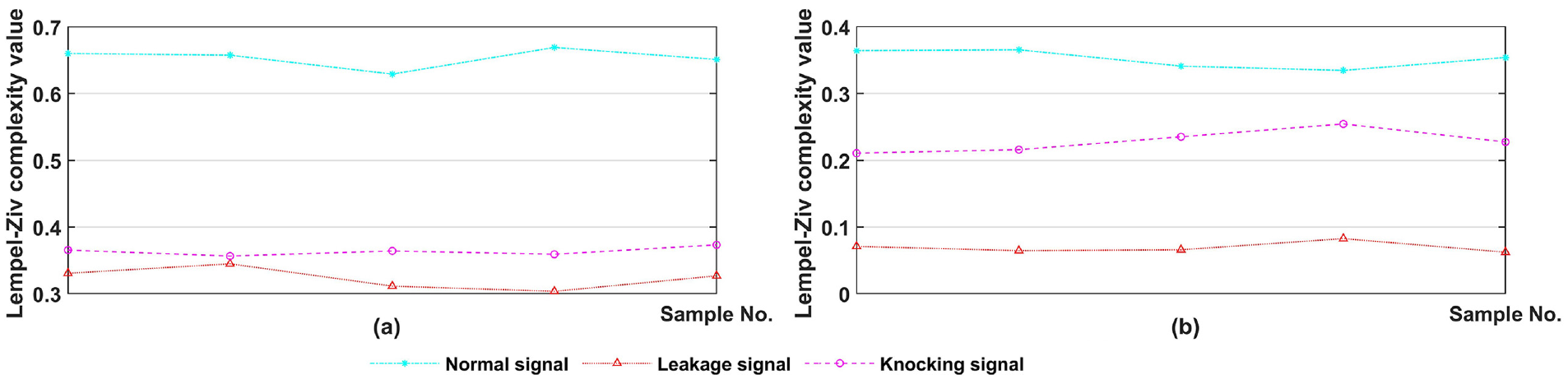
The Lempel–Ziv complexity value of pipeline signal (a) before denoising (b) after denoising.
In order to compare the complexity value of the signal before and after denoising more clearly, 30 groups of experimental samples for each working condition were randomly selected, that is, 90 groups of samples were selected in total, and Lempel–Ziv complexity value of each group was calculated. For the convenience of comparative analysis, the final results are presented in the box plots of Figure 10. Figure 10 shows that the complexity values of pipeline signals after denoising are significantly lower than that before denoising, which is due to the reduction of noise components after denoising, and the reduction of signal randomness, resulting in the reduction of signal complexity. At the same time, it can be observed that the complexity values of leakage signal and knocking signal before denoising overlapped. In contrast, the complexity values of three kinds of signals after denoising do not have any intersection, and the size of the values has obvious difference. The importance of denoising method is proved in this paper, and the Lempel–Ziv complexity index can be used as the characteristic parameter to distinguish different pipeline signals for the subsequent classification and recognition.
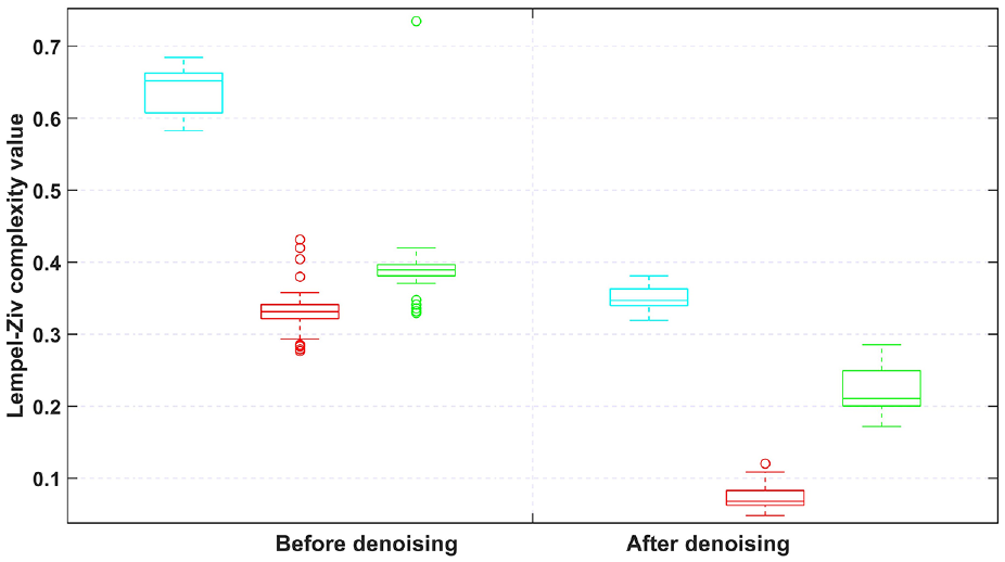
Box plots of the Lempel–Ziv complexity value of pipeline signal before and after denoising (blue box represent the normal signal, red box represent the leakage signal, green box represent the knocking signal, and the circles represent the outliers).
Classification and recognition of pipeline signal based on SVM
For artificial neural network, its construction model requires a large number of sample data, which is not suitable for small samples of pipeline leakage. Decision tree and random forest are very easy to fall into over-fitting. Although a model is generated that fits the training set perfectly, the performance of the model on the test set is very poor (Ferreira et al., 2017). Cortes and Vapnik (1995) proposed the classification algorithm support vector machine (SVM) and compared with the above three pattern recognition methods; SVM adopts a structural risk minimization scheme, which has good generalization ability. In the environment of sparse learning samples, SVM can still maintain high multi-classification accuracy (Jan et al., 2021). In addition, SVM effectively avoids the problems of under-learning, over-learning and local minima, and its robustness is better than other similar related algorithms. It is not affected by external abnormal factors and has good classification effect. Therefore, SVM is used in this study to identify the extracted pipeline feature. Through the pipeline leakage detection platform, 60 groups of each kind of signal were gathered for experiment. Among them, 120 groups of pipeline signals were designed as training samples to train SVM, and the rest 60 groups as testing samples data were input to the trained SVM for prediction. In addition, in order to achieve better classification effect, according to Jia et al. (2019), this study used the PSO to optimally select the parameters (penalty factor c and kernel parameter g) of SVM, and the workflow of PSO-SVM method is shown in Figure 11. Finally, optimum parameters are obtained: penalty factor c = 1.2 and kernel parameter g = 2.17.
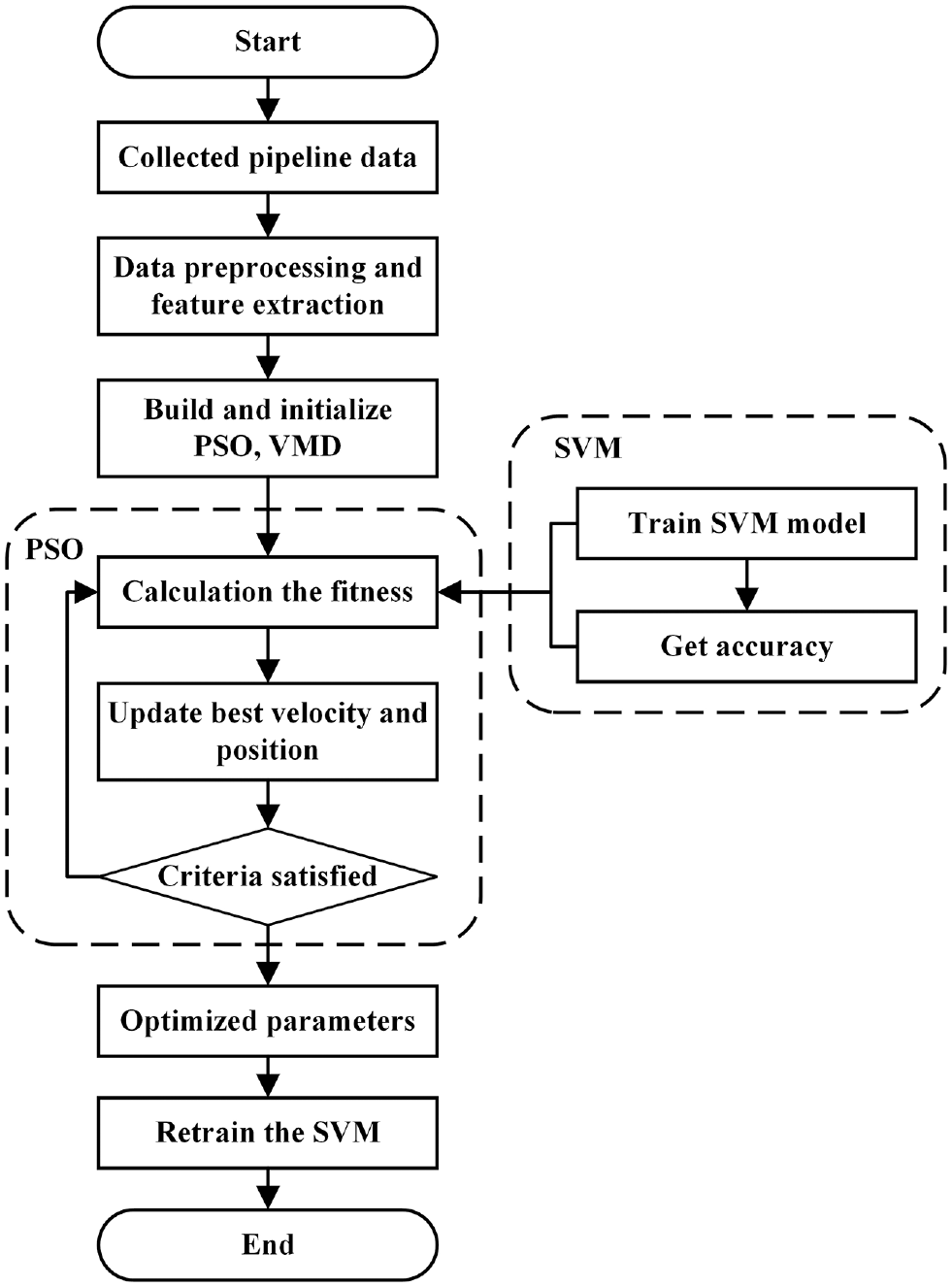
The workflow of PSO-SVM training.
To verify the effectiveness of the proposed method, comparative experiments are designed as shown in Table 11. It shows the comparison of methods, extracted features, and leakage detection recognition rates in the literature. Although these methods have achieved certain detection results, they also have their own shortcomings. For example, the leakage detection model proposed in El-Zahab et al. (2018) can identify the potential leakage size, but there is still the disadvantage that the quality of collected data can be improved by signal filtering. The method proposed in Pérez-Pérez et al. (2021) realized the prediction of leakage location, but the application scope of this method may be limited due to the requirements of pressure flow. As can be seen from the table, the proposed method has the highest recognition accuracy. Compared with other methods, the average identification accuracy is improved by 2.65%, indicating that the proposed pipeline leakage detection method based on improved VMD signal preprocessing and Lempel–Ziv complexity feature selection significantly improved the leakage identification accuracy.
Comparisons of methods, selected features and accuracy of leak detection with other research.
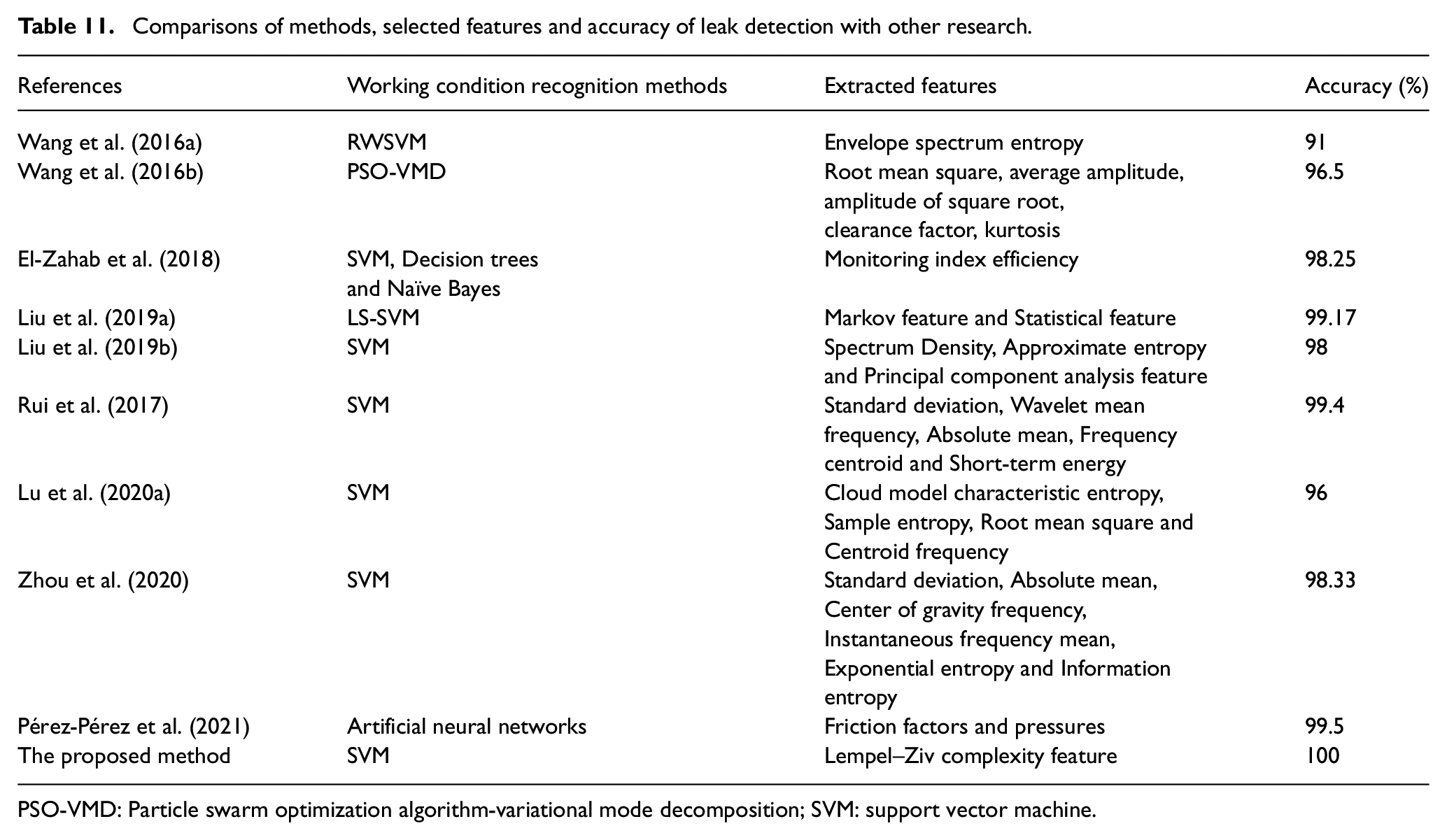
PSO-VMD: Particle swarm optimization algorithm-variational mode decomposition; SVM: support vector machine.
Conclusion
The innovation of this study is to solve the problem of K value selection of VMD using EMD and mutual information, and extract the Lempel–Ziv complexity feature of pipeline signal for leakage detection. In order to solve the difficulty of selecting the K value of VMD by human experience, a method for determining K value based on EMD algorithm and normalized mutual information is proposed. To effectively distinguish the characteristic of the different pipeline signals, Lempel–Ziv index is introduced to measure the complexity of pipeline signals. Compared with other methods in the experiment, the proposed method can improve the detection accuracy and has the higher classification accuracy. Although the proposed leakage detection method effectively improved the accuracy of natural gas pipeline leakage identification, there are still some areas that need to be improved. For example, this study only solved the problem of K value selection and does not further analyze the influence of α value on VMD. Therefore, the main work and research direction in the future is to consider the influence of both K and α on VMD at the same time, and take measures such as studying the new swarm intelligence optimization algorithm and using it to adaptively select the optimal parameter pair [K, α], so that the VMD can achieve the best signal processing effect.
Footnotes
Declaration of conflicting interests
The author(s) declared no potential conflicts of interest with respect to the research, authorship, and/or publication of this article.
Funding
The author(s) disclosed receipt of the following financial support for the research, authorship, and/or publication of this article: The Project Supported by The National Natural Science Foundation of China (NSFC61873058) and (NSFC 51575407), The Natural Science Foundation of Heilongjiang Province (LH2020F005), Youth science foundation project of northeast petroleum university (2018QNL-33), and The Open Fund of The Key Laboratory for Metallurgical Equipment and Control of Ministry of Education in Wuhan University of Science and Technology (MECOF2019B01).