
Abstract
Manifold learning is widely adopted for the fault detection of industrial processes. However, the quality of low-dimensional embedding coordinates can be adversely affected by ill-constructed graph Laplacian. An improved locality preserving projection (ILPP) scheme is proposed. ILPP is built on a geometrically inspired Laplacian, and the Riemannian metric is used to find the suitable bandwidth parameter. The proposed approach combines the advantages of ILPP in preserving manifold data structures and those of support vector data description (SVDD) in handling complex process data distributions. Case studies on helix data, hot strip mill, and Pensim benchmark processes demonstrate the utility and feasibility of the proposed approach. The average fault detection rate for proposed ILPP is 99%, which is higher than locality preserving projection (LPP; 87.8%), local tangent space alignment (LTSA; 74.9%), and principal component analysis (PCA; 90.6%).
Introduction
The progress in industrial processes is resulted in an increase in demand for process safety and reliability. Process monitoring can ensure safe operation of the plant by earlier detection and management. With the advancement in software and hardware technologies, large amounts of data are collected for multivariate statistical process monitoring (MSPM) (Chong et al., 2020; Guo et al., 2019). MSPM methods aim to seek the intrinsic relationship among variables. Dimensionality reduction has become a fundamental premise for most data-driven approaches due to the intrinsic features of process data, which are non-linearity, high-dimension, and complicated connection among process variables (Yin and Yan, 2021). Dimensionality reduction aims to condense high-dimensional data into a relatively small set of variables, while retaining the original data structure (Lu et al., 2021).
There are two major research directions based on the data structure. The first direction considers a single structure of entire process data, that is, global or local. Principal component analysis (PCA), partial least square (PLS), and independent component analysis (ICA) capture the global structure of the data (Basha et al., 2020). PCA is the widely adopted technique in actual industrial processes due to its concise derivation and easy implementation. PCA only captures the global structure of the original dataset through preserving variance information. Nevertheless, the industrial process data are often considered as time series, containing local geometric structures (Bounoua et al., 2020). Therefore, significant information is lost, resulting in unsatisfactory monitoring results. This limitation has prompted the construction of more complicated and non-linear methods underneath the framework of manifold learning.
Manifold learning offers a different viewpoint based on the interpretation of data lying on a manifold, embedded in a much higher dimensional space (Chen et al., 2019). The main idea of manifold learning is to seek local neighborhood structure, such that, the geometric features and characteristics of the manifold data are retained in low-dimensional subspace (Orzechowski et al., 2020). These techniques are often referred to as spectral embedding methods (Ayesha et al., 2020). They include, among others, isometric feature mapping (Isomap) (Tenenbaum et al., 2000), local tangent space alignment (LTSA) (Dong et al., 2020), Laplacian eigenmaps (LEs) (Wang, 2012), local linear embedding (LLE) (Li et al., 2019), locality preserving projection (LPP) (He and Niyogi, 2004), and neighborhood preserving embedding (NPE) (He et al., 2005). Among all, LPP and NPE are in wide usage for data-driven process monitoring (He et al., 2018). Because they can generate a detailed map, which is linear and can easily be obtained like PCA. Several variations have been proposed to classical LPP and NPE (Guo et al., 2022; Yao et al., 2022), such as improved local entropy locality preserving projections (ILELPP; (Guo et al., 2019), which forms the local entropy LPP. The method removes the non-Gaussian characteristics using entropy LPP and showed improved process monitoring.
The second approach is inspired by the idea of combining PCA with LPP or NPE to use both global and local information. Inspired by this, Zhang et al. (2011) proposed global–local structure analysis (GLSA), combining PCA with LPP for fault detection. Yu (2012) proposed local and global PCA (LGPCA) by considering both the local and global information. Following this novel approach, several new methods have been formulated (He and Xu, 2016; Luo et al., 2016; Tong and Yan, 2014; Zhan et al., 2019) recently. The major difference among these methods is located in a way; they integrate the objective function of PCA and LPP. Similarly, Chen et al. (2019), Cui et al. (2021), Miao et al. (2015), and Tan et al. (2019) combine PCA with NPE. These new manifold learning methods showed significant improvement in fault detection performance.
Despite all the advances mentioned above, there are still some gaps in these methods (Orzechowski et al., 2020; Perraul-Joncas and Meila, 2017; Shah et al., 2022). The most important criticism is that manifold learning methods fail to reveal underlying geometric structure in many cases (Perraul-Joncas and Meila, 2017). Our motivation focuses on geometrical aspects of process data through manifold learning. Almost all the manifold learning methods are constructed based on graph Laplacian
The significance of this method is that, First, it provides a framework to construct a geometrically inspired Laplacian, which is critical in all manifold learning settings. Second, support vector data description (SVDD) is adopted, as it can handle more complex process data distributions than traditional statistical tools. The diagram of the improved locality preserving projection (ILPP) method is shown in Figure 1.
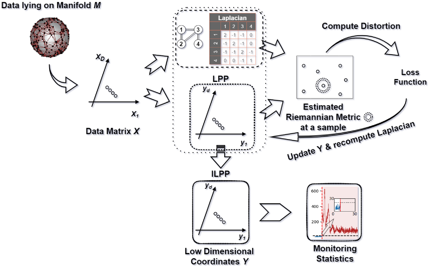
Diagram of the ILPP method.
The contributions and novelties are listed as follows:
To overcome the problem of geometric distortion in existing manifold learning literature, the paper put forward ILPP-based manifold learning method using Riemannian metric.
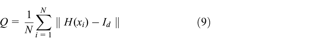
A novel qualitative metric for comparing the obtained embeddings with desired embeddings is discussed. In particular, when the Riemannian metric converges to the unit matrix, the geometric distortion is minimized.
The concept behind ILPP is general and has the potential to be extended to Laplacian-based manifold learning methods; however, this work is limited to the LPP.
In addition to fault detection of the hot strip mill process (HSMP) and the Pensim benchmark process, ILPP is applied for feature extraction of the Helix data. Experimental results are validated using the three different quality indices.
The remainder of the paper is structured as follows. The “Preliminaries” section provides preliminary information, which is followed by the core ideas of manifold and graph Laplacian. Details about our proposed framework are discussed in the “Algorithm formulation” section, which includes LLP, Riemannian metric estimation, computing bandwidth
Preliminaries
The central theme of manifold learning relies on the manifold assumption, which states that data exist on a low-dimensional manifold embedded in higher dimensional Euclidean space. The Riemannian metric embodies the geometry of the underlying manifold. Following that, some related concepts are defined, used in this research work.
Riemannian manifold
Formally, consider a Riemannian manifold
Graph Laplacian
Graph Laplacian
Mathematically, consider the
where
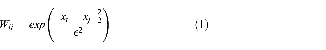
The problem to compute
Following equation (1), the similarity

where
Algorithm formulation
LPP
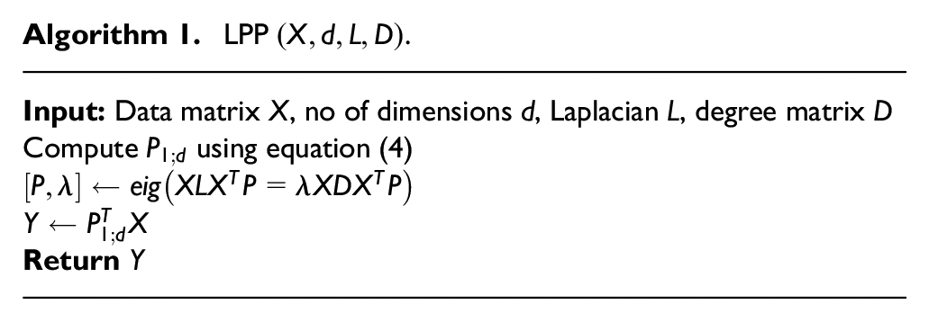
LPP is a linear dimensionality reduction method that uses data points to generate an adjacency map (He and Niyogi, 2004). Then, the graph Laplacian
Construct an adjacency graph: Let
Calculate weighted graph Laplacian: Construct a weighted graph Laplacian as described in the “Graph Laplacian” section. The most important parameter is bandwidth
Compute projection matrix: Projection matrix

The eigenvalue decomposition of equation (4) generates the eigenvector

Rest of the LPP method is summarized in Algorithm 3.1 as adapted from He and Niyogi (2004).
Computing the Riemannian metric
Riemannian manifold
Following the work of Perraul-Joncas and Meila (2017), Riemannian metric

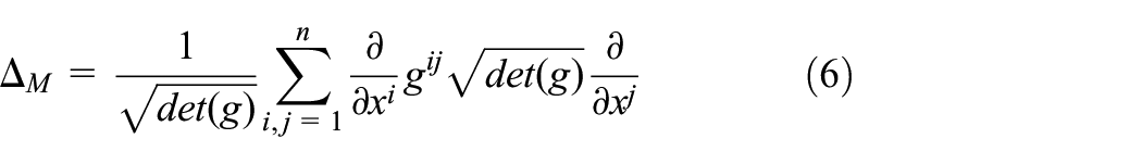
In the differential geometry, there is a powerful proposition that states that the graph Laplacian
Laplacian
Given the input data matrix
From the perspective of matrix notation, the Jacobian
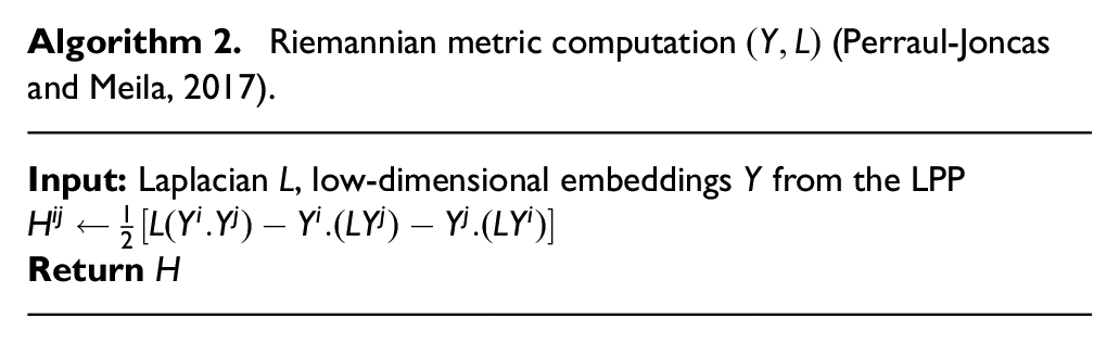
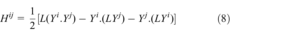
To this end, the method to compute the Riemannian metric using graph Laplacian and low-dimensional embeddings has been discussed.
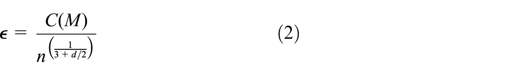
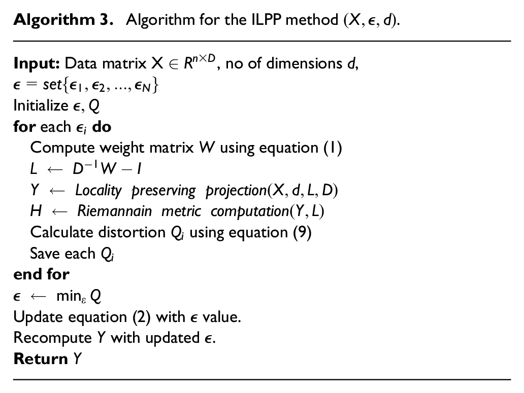
Computing bandwidth for Laplacian
Riemannian metric is a powerful tool because of the fact, that it embodies the manifold geometry. Whereas, Laplacian
The good value for bandwidth

Algorithm 3, provides a framework to compute bandwidth
Quality indices
In this work, we consider three different evaluation metrics to justify the integrity of proposed ILPP approach.
However, continuity
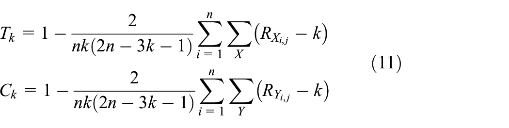
The
Process monitoring model based on the ILPP
The idea of the SVDD is based on the one-class classification (Yuan et al., 2020). It seeks to find the lowest volume hyper-sphere in a high-dimensional ambient space that encompasses the majority of the fault-free data. However, during the faulty event, the fault data reside outside the hyper-sphere (Huang and Yan, 2016).
In industrial process, relationship among process variables are quite complex. Some industrial variables can be linearly related, whereas others are non-linearly to each other and similarly, some variables are independent or not correlated with each other. In comparison to the classical statistical tools, SVDD can handle more complex data distributions and relationships among different process variables (Li et al., 2021).
Mathematically, consider
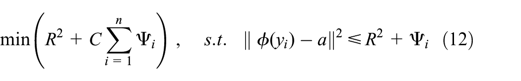
where
where
Linear:
Polynomial:
RBF:
Gaussian:
Sigmoid:
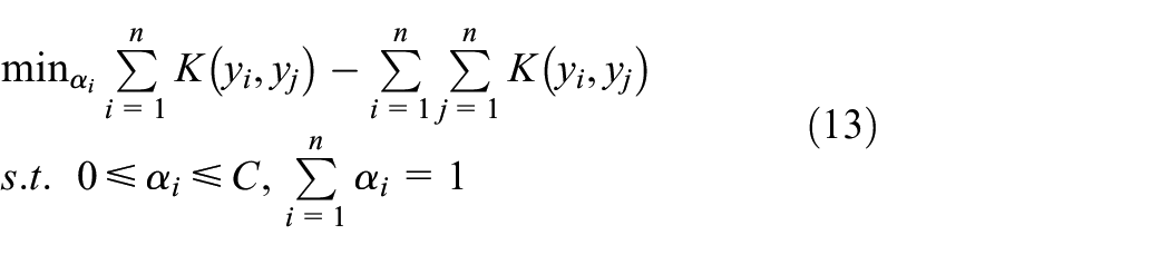
where
Following equation (13), the suitable solution of
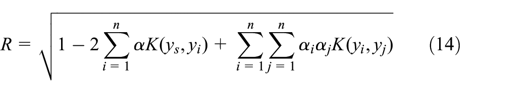
where
Consider
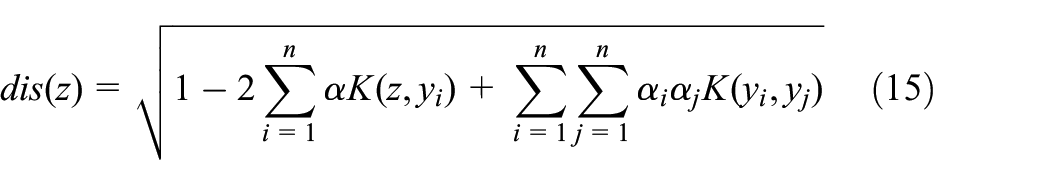
The process monitoring model is developed based on equation (15). The monitoring statistics

In summary, low-dimensional embedding coordinates
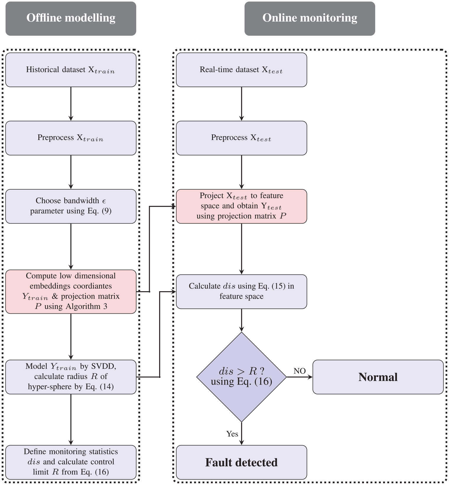
Flow chart of the ILPP method.
Monitoring procedures
Monitoring procedure is described as follows:
Offline modeling:
Step 1: Normalize the training data
Step 2: Choose the bandwidth
Step 3: Generate low-dimensional embedding coordinates
Step 4: Setup monitoring model based on SVDD and calculate radius
Step 5: Define monitoring statistics
Online monitoring:
Step 1: Normalize testing data
Step 2: Compute testing sample embedding coordinates
Step 3: Calculate
Step 4: Compare results against the
Experimental verification
The simulation results consider three case studies from two different industrial processes. First case is fault detection of real HSMP. Whereas, second and third case studies are related to fault detection of fouling faults in steam turbine system. Before proceeding further, it is important to define evaluation criteria for our method.
Case study 1—helix synthetic data
Consider toroidal helix dataset with manifold dimension in higher dimensional ambient space with
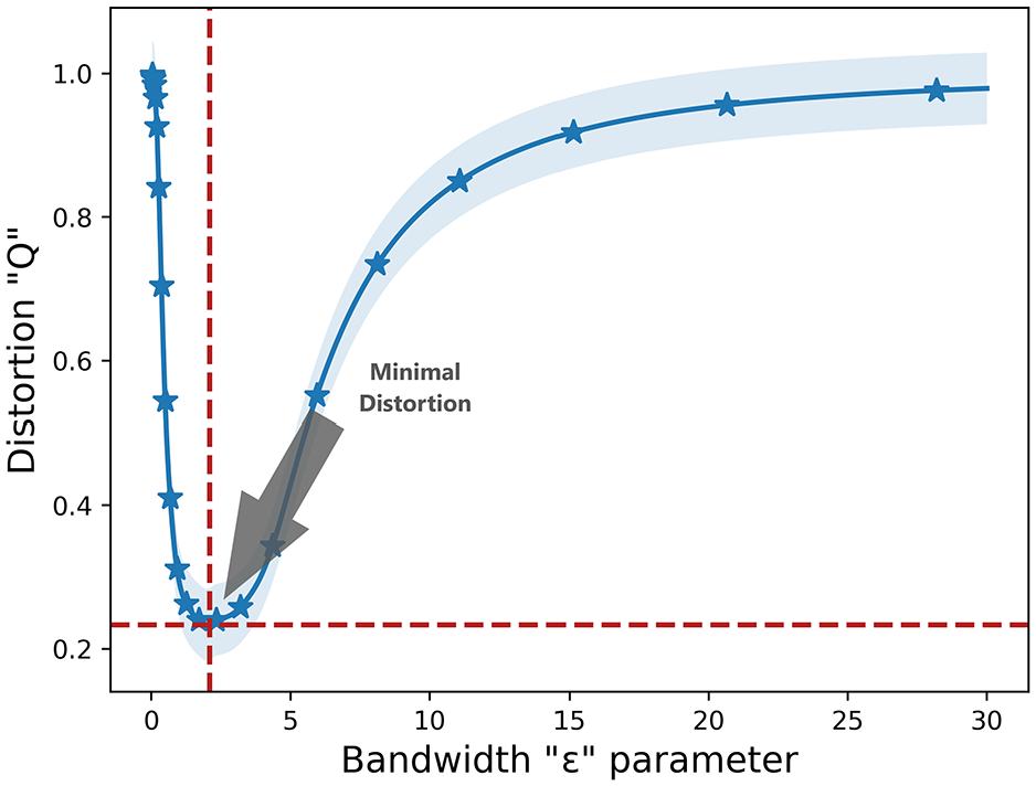
Distortion versus bandwidth parameter for the helix data.
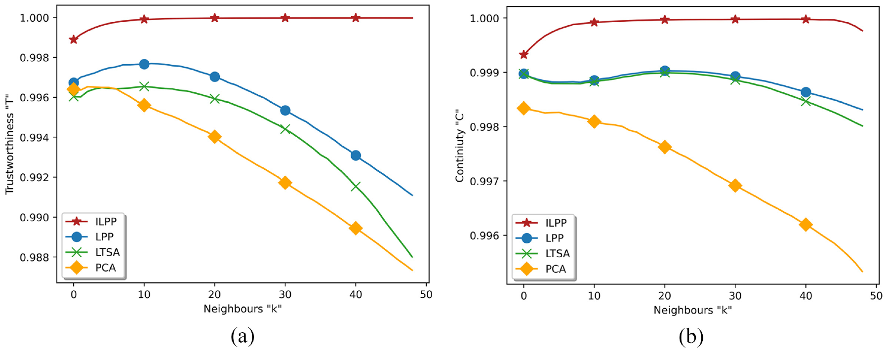
Trustworthiness and continuity against four different methods for the helix data: (a) trustworthiness and (b) continuity.
The low-dimensional projections based on the ILPP, LPP, LTSA, and PCA are demonstrated in Figure 5. Data points are colored differently in each subplot based on their locations. The projected samples are not separated by LPP, LTSA, or PCA. ILLP, on the other hand, is able to successfully separate the samples. More importantly, the ILPP results closely resembled the desired projections.
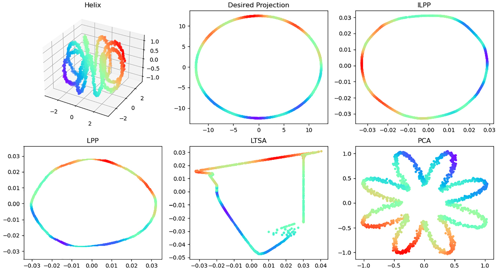
The 2D projections of 3D helix data using four different methods.
Case study 2—HSMP
The HSMP is steel manufacturing process (Zhang et al., 2019), which is fully automated. Thus, the real-time monitoring of this process is required to ensure highest efficiency and consistent production. The schematic for the HSMP is illustrated in Figure 6.
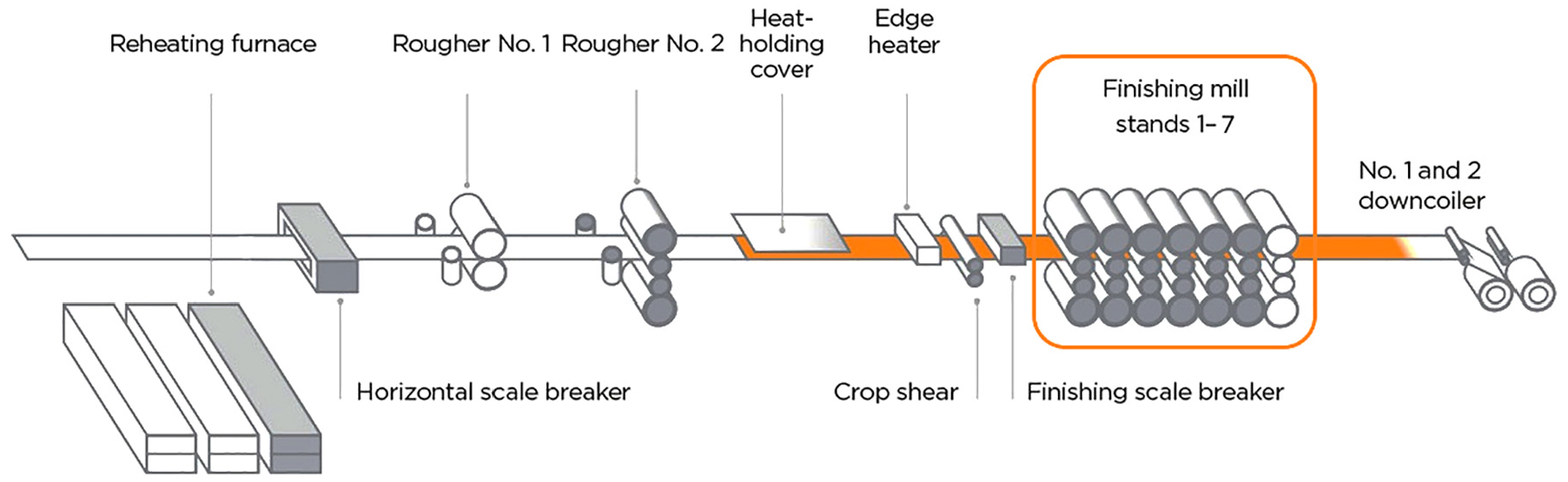
The hot strip mill process schematic.
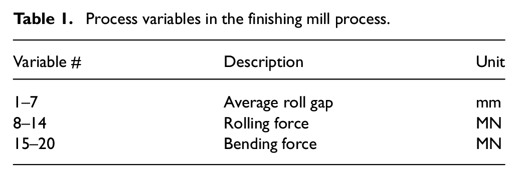
The finishing mill process (FMP) is an essential part in HSMP because it guarantees the continuous operation, consistency, and higher accuracy of the end product. A typical FMP constitutes seven stands. Each stand is made up of two working rolls in center and both sides of each stand include the two supporting rolls. Furthermore, hydraulic system is adopted in each stand to generate rolling and bending forces to achieve the optimum strip thickness. FMP is made up of 20 variables. Table 1 lists the process variables.
Process variables in the finishing mill process.
This case study utilizes FMP to illustrate the efficacy of the ILPP approach proposed here. The finished strip thickness is the most critical consideration in determining the product quality. For modeling and monitoring purposes, two different sets of data with 3500 samples each belonging to normal and faulty operation are collected with a sample rate of 10 ms. The gap control loop fault in the
The distribution of first 15 process variables in FMP dataset is shown in Figure 7. The results verified that the variables follow non-Gaussian distribution. SVDD model is adopted considering the non-Gaussian distributions present in that dataset. The model is constructed on low-dimensional embeddings space based on the “Process monitoring model based on the ILPP” section and Gaussian kernel K is adopted as well.
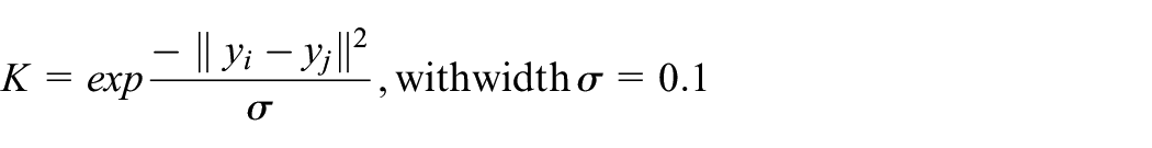
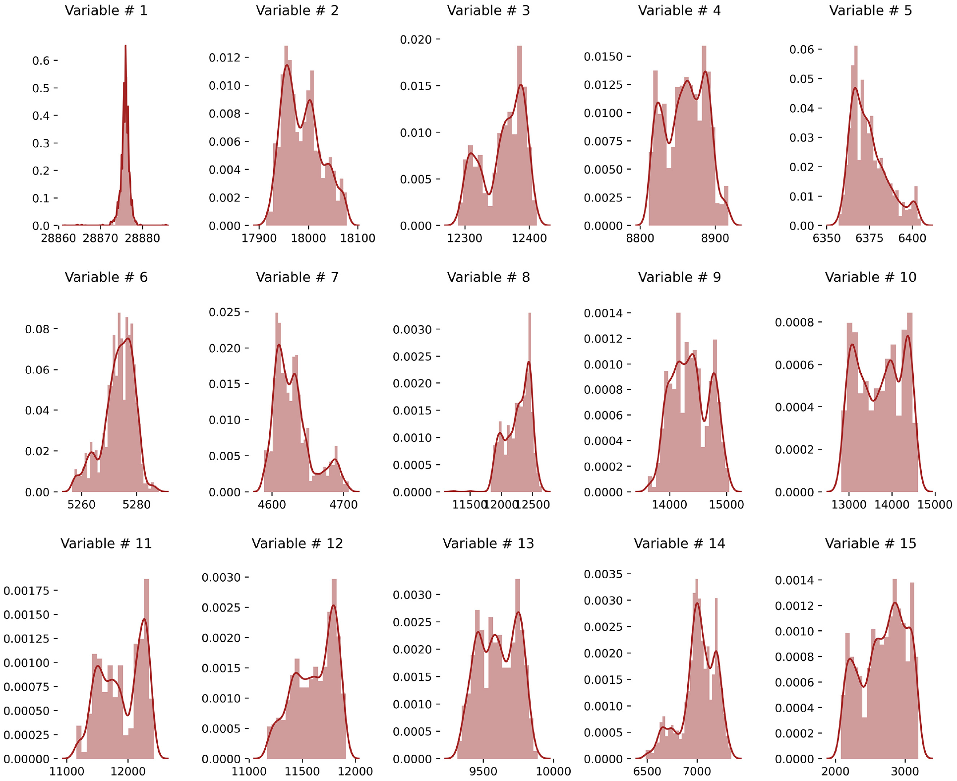
The distribution of process variables in the finishing mill process.
LPP, LTSA, and PCA are chosen as comparison methods. It is important to mention that, all of these manifold learning methods are implemented in python environment with their standard parameters and Gaussian kernel is chosen to develop SVDD model, identical to the one adopted for our proposed ILPP.
Before proceeding, it is essential to determine the intrinsic dimension (Einbeck et al., 2020) for the FMP data. Contrary to the cumulative percentage variance (which is commonly used for PCA), dimensionality from angle and norm concentration (DANCO; Ceruti et al., 2014) is utilized in computing the suitable number of dimensions for lower dimensional space. In case of FMP, we choose number of dimensions to be “3” for improved LPP method. Similar to the “Case study 1—helix synthetic data” section, lowest distortion is achieved against
Fault of gap control loop
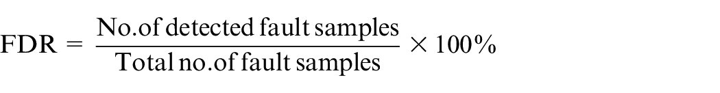
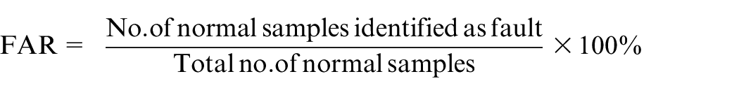
This fault has direct impact on finished thickness of strip. It jumps to higher value as shown in Figure 8. To have the faithful comparison, the results based on SVDD statistics are constructed. The fault detection rate (FDR) and false alarm rate (FAR) are defined as follows
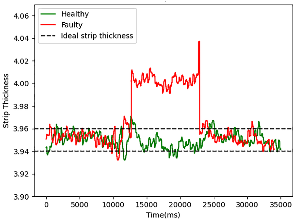
The thickness of during healthy and faulty conditions.
Process monitoring statistics from the four-dimensionality reduction methods, which are LPP, LTSA, and PCA, are illustrated in Figure 9. All the faults are detected by the proposed ILPP approach with highest FDR closer to 99%. In addition FAR value is satisfactory and closer to 0.17%. However, other methods produce poor results comparatively. The results based on FDR and FAR values are listed in Table 2.
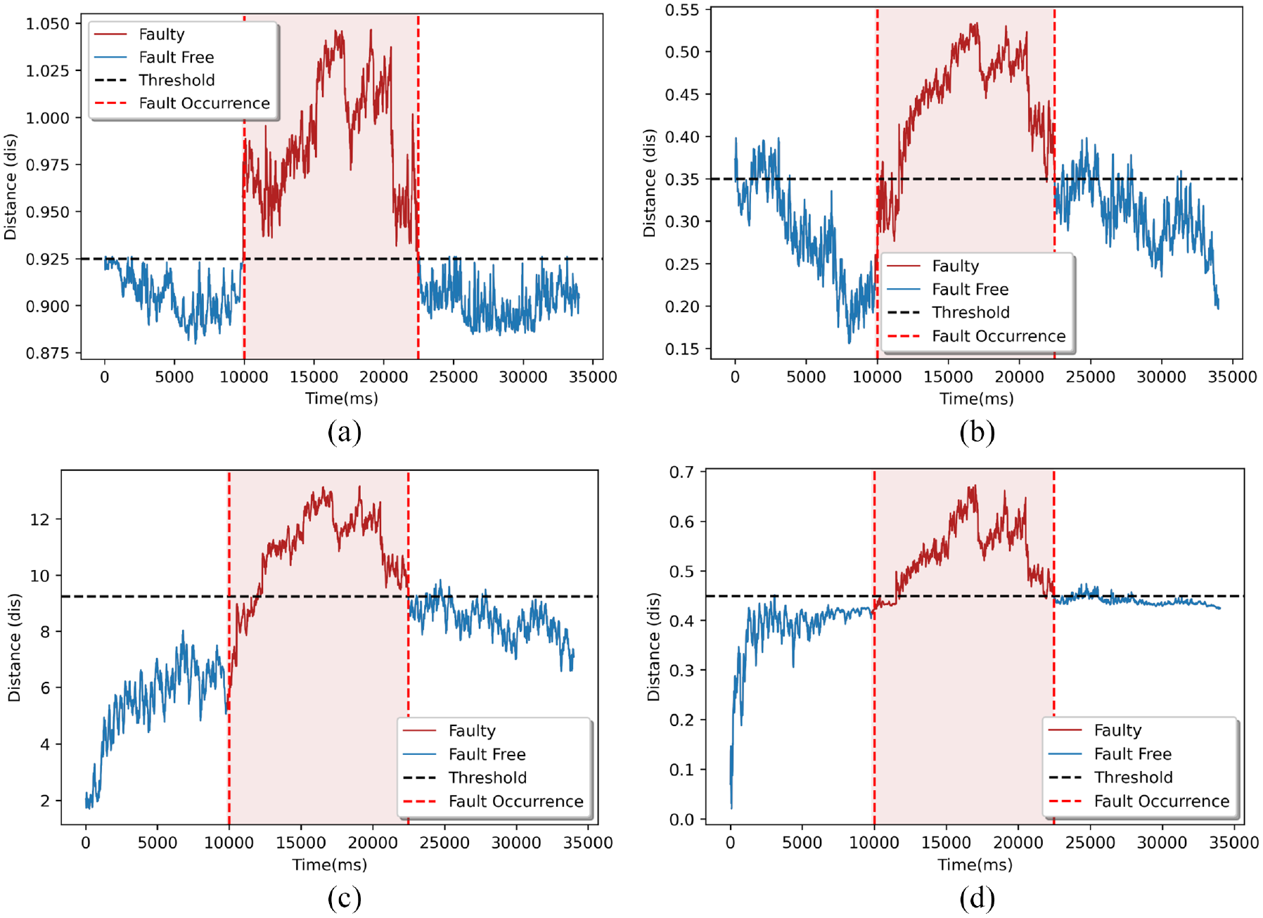
Monitoring charts for the fault of gap control loop: (a) ILPP, (b) LPP, (c) LTSA, and (d) PCA.
Fault detection rate/false alarm rate of the finishing mill process (%).
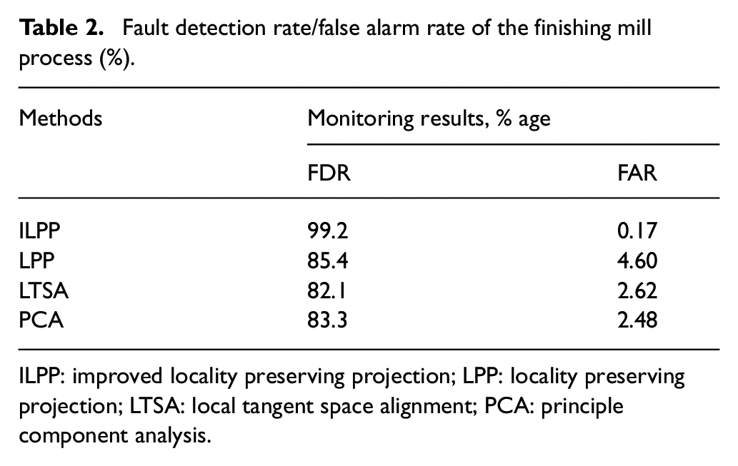
ILPP: improved locality preserving projection; LPP: locality preserving projection; LTSA: local tangent space alignment; PCA: principle component analysis.
Case study 3—Pensim benchmark process
Pensim is a widely adopted non-linear chemical process for penicillin manufacturing. The schematic of Pensim benchmark process is demonstrated in Figure 10 and it has often been applied to fault detection (Peng et al. 2020). The process consists of two main operating regions: (a) the pre-culture and (b) batch feeding. The first region takes 50 hours and the second region consumes 350 hours in total. Therefore, the total simulation time for the entire penicillin fermentation process is 400 hours.
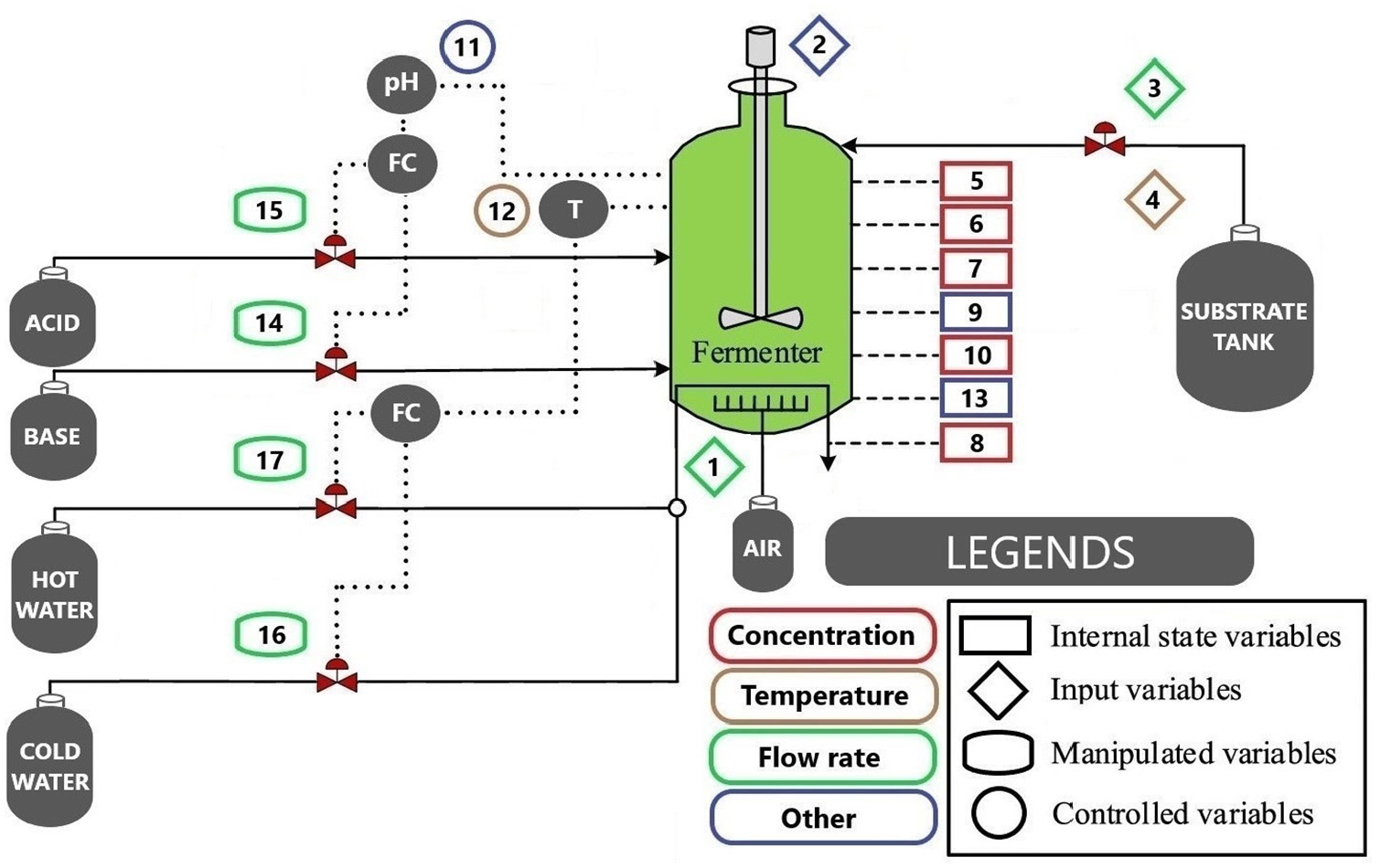
The Pensim benchmark process schematic.
The Jarque–Bera (JB) (Thadewald and Büning, 2007) test function in Python is used to verify the non-Gaussian distribution of Pensim process variables. The JB test returns two values, which are JB statistic and corresponding p-value. If JB statistic = 0, it means that the variable obeys the Gaussian distribution, else the non-Gaussian distribution. Whereas, the p-value is the probability value of accepting the hypothesis. If the p-value is closer to 0.05, then the data reject the hypothesis of Gaussian distribution. The verification results are shown in Table 3. All the variables obey the non-Gaussian distribution except the substrate feed temperature variable. Since the penicillin fermentation process has non-Gaussian characteristics (Peng and RuiWei, 2021), the SVDD-based fault detection is adopted in this work.
JB test result of process variables in the Pensim benchmark process.
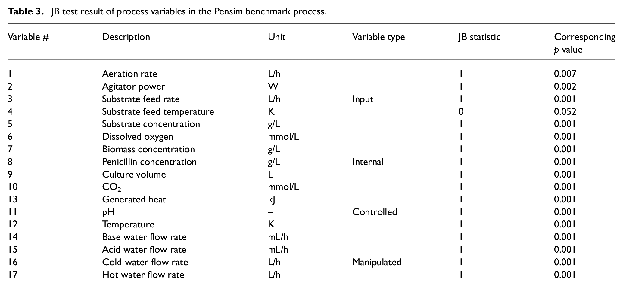
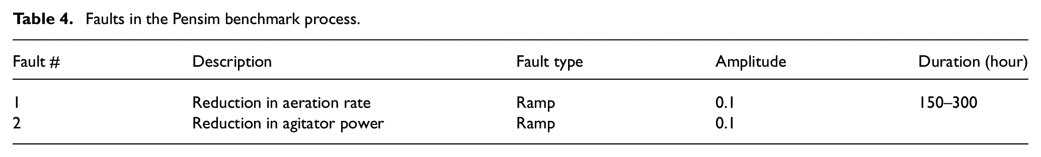
The process simulation is performed using the software Pensim V2.0. It contains 17 variables, as listed in Table 3. Two datasets are collected based on normal and fault conditions, each set consist of 400 hours with a sampling time of 0.1 hour. Two fault conditions are considered in the simulation example. A ramp fault with an amplitude of 0.1 is added in variables 1 and 2 for a total duration of 150 hours from 150 to 300 hours. Faults description is given in Table 4.
Faults in the Pensim benchmark process.
The ILPP is adopted to develop a fault detection model. Then, SVDD model is constructed following the “Process monitoring model based on the ILPP” section and Gaussian kernel is adopted. The fault detection results based on proposed ILPP are compared with LPP, LTSA, and PCA.
Fault 1 is ramp disturbance that causes a reduction in aeration rate. Figure 11 demonstrates the monitoring chart of all the methods. The proposed ILPP successful identifies all the faults with highest FDR closer to 99.9%. In case of LPP, the fault was initially detected at 170th hour. Therefore, its FDR lies at 85.6%. Monitoring results based on LTSA illustrate the poor FDR in comparison to the rest of dimensionality reduction methods. Finally, in the case of PCA, FDR of 89.5% is comparable to that of the proposed ILPP method. However, FAR is highest among other methods. The monitoring results based on four-dimensionality reduction methods are listed in Table 5.
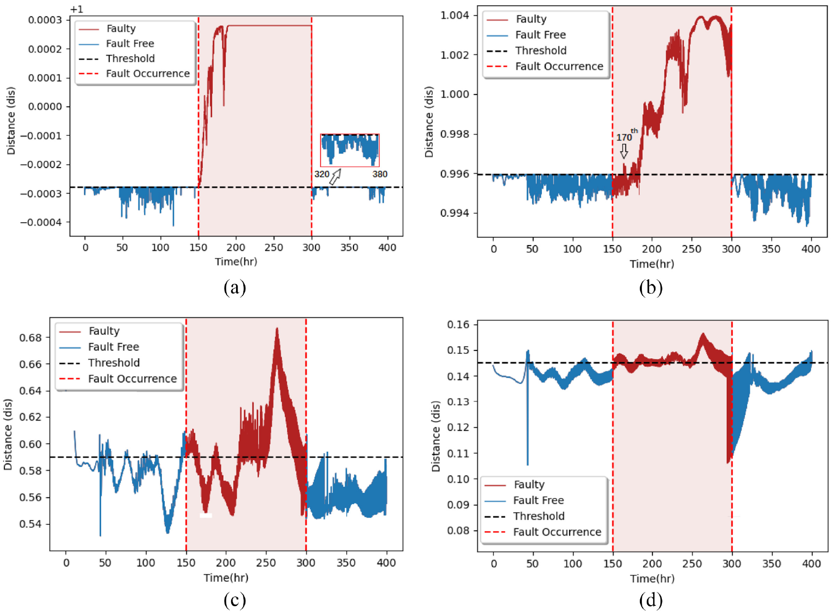
Monitoring charts for the Pensim benchmark process—fault 1: (a) ILPP, (b) LPP, (c) LTSA, and (d) PCA.
Fault detection rate/false alarm rate of the Pensim benchmark process (%).
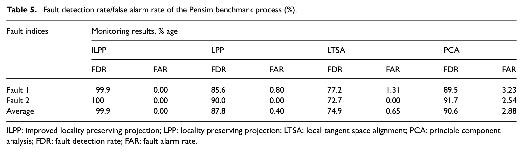
ILPP: improved locality preserving projection; LPP: locality preserving projection; LTSA: local tangent space alignment; PCA: principle component analysis; FDR: fault detection rate; FAR: fault alarm rate.
Similar to fault 1, fault 2 is a ramp disturbance that causes a reduction in agitator power. Monitoring chart for all the methods is illustrated in Figure 12. The proposed ILPP identifies all the faults with FDR at 100%. In case of LPP, the fault was initially detected at 160th hour. Therefore, its FDR lies at 90%. Monitoring results based on LTSA demonstrate the worst FDR at 72% compared to the rest of dimensionality reduction methods. Finally, in case of PCA, FDR of 91% is comparable to that of proposed ILPP method. However, the FAR produces by PCA method is highest in comparison to other methods. The monitoring results based on four different methods are also listed in Table 5.

Monitoring charts for the Pensim benchmark process—fault 2: (a) ILPP, (b) LPP, (c) LTSA, and (d) PCA.
In summary, the ILPP demonstrates the improved fault detection. After ILPP, PCA produces better FDR and FAR scores. The average scores based on both the faults against all four methods are also listed in Table 5. The ILPP produces the best average compared to the rest of the methods.
The significant advantage to the proposed ILPP method based on Riemannian metric is that we can extend this approach to several other manifold learning methods that use graph Laplacian as their building block and compute its geometrically inspired bandwidth
Conclusion
This paper proposed a fault detection approach that departs from existing manifold learning literature in process monitoring. It is motivated by geometrical aspects of the data, which are typically ignored or poorly understood in most cases. There are some notes to be pointed out. First, through this approach, the ILPP is developed using geometrically inspired graph Laplacian, and bandwidth parameter for Laplacian is computed through Riemannian metric. Second, the approach can be applied to a wide variety of manifold learning methods that rely on Laplacian as their preliminary step. Third, ILPP is combined with SVDD to handle complex process data distributions. The effectiveness of ILPP is demonstrated through the feature extraction of the helix data and fault detection of the HSMP and the Pensim benchmark process. The quantitative results demonstrate the method’s superiority compared to the other methods. A few limitations of the ILPP are higher computational complexity
Footnotes
Declaration of conflicting interests
The author(s) declared no potential conflicts of interest with respect to the research, authorship, and/or publication of this article.
Funding
The author(s) received no financial support for the research, authorship, and/or publication of this article.