
Abstract
In this article, an experimentally validated new mathematical model is developed to show a vacuum box electric furnace’s thermal behavior and predict the temperature of the desired point inside it. The model is derived by extracting the equivalent electrical circuit of the system based on heat transfer principles. To show the accuracy of the model, its behavior has been evaluated by comparing it with experimental data. Then, an optimized fuzzy controller is designed using four metaheuristic algorithms, that is, genetic algorithm, harmony search, cuckoo optimization algorithm, and water cycle algorithm. The rule-base and the membership functions are optimized by these optimization algorithms with four criteria, that is, integral of absolute error, integral of square error, integral of time absolute error, and integral of time square error. The simulation results indicate that the fuzzy controllers tuned by the integral of time square error criterion get better performance, especially in genetic and water cycle algorithms. The designed controller based on the proposed model is implemented on an experimental setup. The experimental test shows a good agreement between experimental and simulation results. The obtained results show the ability of the fuzzy controller and approve that the developed model can be used for transient performance analysis of a vacuum box electric furnace and real-time controller design.
Keywords
Introduction
Vacuum furnaces and ovens have many applications in industry for doing metallurgical processes on a specimen for enhancing its characteristics (Hao et al., 2008; Tudon-Martinez et al., 2019; Zimmermann et al., 2012). In the food industry for drying food, it is needed to make vacuum conditions (Hosseinpour and Martynenko, 2020). Electronic components, semiconductors, and medications are heat sensitive and are damaged by the conventional drying processes. Delicate drying processes are done in vacuum drying furnaces and ovens because the boiling point is reduced in a vacuum environment (Hosseinpour and Martynenko, 2020). For example, flammable solvents suppression and drying tiny parts are in the category of the delicate drying process. Diminishing oxidation during this process is done in a low-pressure environment.
In these systems, stabilizing the system to the desired temperature all along the process with no steady-state error, less rise time, and overshoot is necessary. Moreover, the system should be robust against uncertainties and disturbances. Since these systems are in dealing with many uncertainties and disturbances, achieving the desired control performance is hard using traditional control methods.
Until now, many attempts have been taken to design temperature controllers such as proportional–integral–derivative (PID), fuzzy, and some nonlinear controllers. In Rashid et al.’s study (2016), a multi-rate modeling and economic model predictive control (MPC) was considered for electric arc furnaces. However, the MPC strategy needs a very accurate model of the system. But, the parameters of these systems, such as heat transfer coefficients, may change due to environmental conditions.
Many control strategies such as linear quadratic regulator (LQR) optimal control, adaptive control (Gholami-Khesht et al., 2021a), MPC (Zou and Wang, 2019), sliding mode control (Gholami-Khesht et al., 2021b), and so on are model-based, and their computational costs are high. The linear optimal control strategies such as LQR are suitable for linear systems and have good performance only around the working point. Using Pontryagin’s maximum principle to design an optimal controller is failed due to the highly nonlinear models of furnaces. This problem also exists in designing an adaptive controller. Other model-based controllers have the same problems.
The most used controller in the industry is PID which has many restrictions due to its linearity (Wang and Liu, 2021). It is shown that the challenges in electric vacuum furnaces such as nonlinearity, delay, and time-varying can be somewhat solved using the genetic algorithm (GA)-PID controller (Lu et al., 2012). In Gani et al.’s study (2019), an optimal PID controller was designed to control the temperature of the vacuum furnace. The other methodology is robust fractional PID implemented in solar furnaces (Beschi et al., 2016), which is a nonlinear controller.
Due to the weakness of model-based controllers in highly nonlinear and uncertain systems, this paper aims to propose a non-model-based control strategy with robust performance to reduce rise time and overshoot. The fuzzy controller mimics the behavior of an expert in regulating the behavior of the system. So, it not only does not need the model of the system but also is robust due to acting based on the logic of the system.
A fuzzy controller is used to control the indoor temperature to improve the indoor environment’s thermal comfort and achieve an energy saving of air-conditioning system (Li et al., 2021). And also, fuzzy controller applications include fuzzy control design for industrial rotary drying systems and controlling load frequency in power systems (Gheisarnejad and Khooban, 2019; Júnior et al., 2020). Moreover, the combination of fuzzy and model predictive was used to control the temperature of the inner tube fluid of a heat exchanger (Mazinan and Sadati, 2010).
However, deriving optimal rules and membership functions is challenging in fuzzy controller design. These problems can be solved using metaheuristic algorithms. In this paper, different metaheuristic algorithms are used for optimizing the fuzzy controller and their results are compared.
For understanding the heat transfer process in a furnace and also for designing a temperature controller, a mathematical model is useful. Modeling the heat transfer systems like ovens and furnaces has three common targets:
Optimization.
Designing a temperature controller.
Assessment of the furnace performance before experimental tests.
Three-dimensional (3D), two-dimensional (2D), zero/one-dimensional, state-space, and transfer function models were presented for heat transfer environments. In 3D and 2D models, the computational fluid dynamics (CFD) method is often used. Although these models have high precision results in showing the heat transfer process inside a furnace, the processing time is high (De Castro et al., 2002; Hao et al., 2008; Mayr et al., 2018; Tang et al., 2017). So, they are not suitable for real-time controller design.
To overcome the problem of computational cost, the zero/one-dimensional models have been presented. These models use energy balance equations for describing heat transfer environments (Tudon-Martinez et al., 2019). The state-space model by Almutairi and Zribi (2015) and transfer function model (Gani et al., 2019; Liu et al., 2014; Sinlapakun and Assawinchaichote, 2015) were used to design a temperature controller. In this paper, a new state-space model is developed for a vacuum box electric furnace for the first time, which is suitable for controller design and real-time application.
The main contributions of the paper are as follows:
A new experimentally validated nonlinear ODE model for a vacuum box electric furnace is presented using the heat transfer principles. The model is presented in the state-space form to be useful for controller design.
A fuzzy controller is designed and its membership functions, rules, and gains are optimized using four metaheuristic algorithms, that is, GA, harmony search (HS), cuckoo optimization algorithm (COA), and water cycle algorithm (WCA) which their application in this problem is new.
For each metaheuristic algorithm, four criteria are regarded. Then, the performance of the fuzzy controller in each optimization algorithm is compared.
The designed controller is implemented on the experimental setup. The experimental tests show that the proposed model and controller are valid and can be used for other purposes.
The structure of the article is along these lines. In the next section, the mathematical model of the system is developed using heat transfer principles. In section “Experimental setup,” the experimental setup is described in detail, and the validation between the mathematical model and experimental data is presented. In section “Controller design,” the fuzzy controller is designed using four metaheuristic algorithms. The performance of the controller and the metaheuristic algorithms are discussed in section “Results and discussions.” Moreover, the experimental implementation of the designed controller is shown in this section. Finally, the conclusion and future works are presented.
Model development
System description
The geometry of the system is shown in Figure 1. The furnace has a cubic shape. The plates are stainless steel (AISI 304). The side plates have the areas A1–A6, respectively. As mentioned, the oven works in a vacuum condition, so the heat transfer inside the system is radiation. The exerted thermal flux by heaters is possible through plates 1, 2, 3, and 4. Heat fluxes through plates 1–4 are shown by q1–q4. Between each plate and the environment is an insulator. The heat transfer between each insulator and the environment is convection. The heat transfer mode, along with the insulators, is conduction.
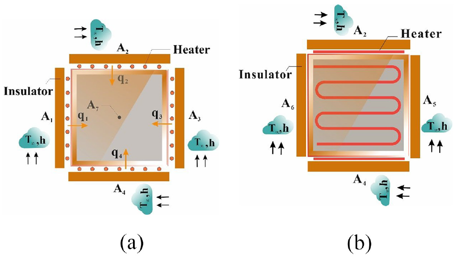
The geometry of the system and the position of the heaters and thermocouples (a) front view and (b) side view.
To study the temperature variation of a node inside a vacuum environment, a spherical node in the middle of the system is considered (Figure 1(a), Point
State-space model
Since the aim is to calculate the heat flux exerted to the desired point in the furnace, the formulation “equivalent electrical circuit” is used, which this type of formulation and method has not been used for vacuum box furnaces so far. The electrical circuit of the system based on Figure 1 is shown in Figure 2. As we can see in this figure, seven nodes state the six plates and the spherical point inside the furnace (J1,…,J7).
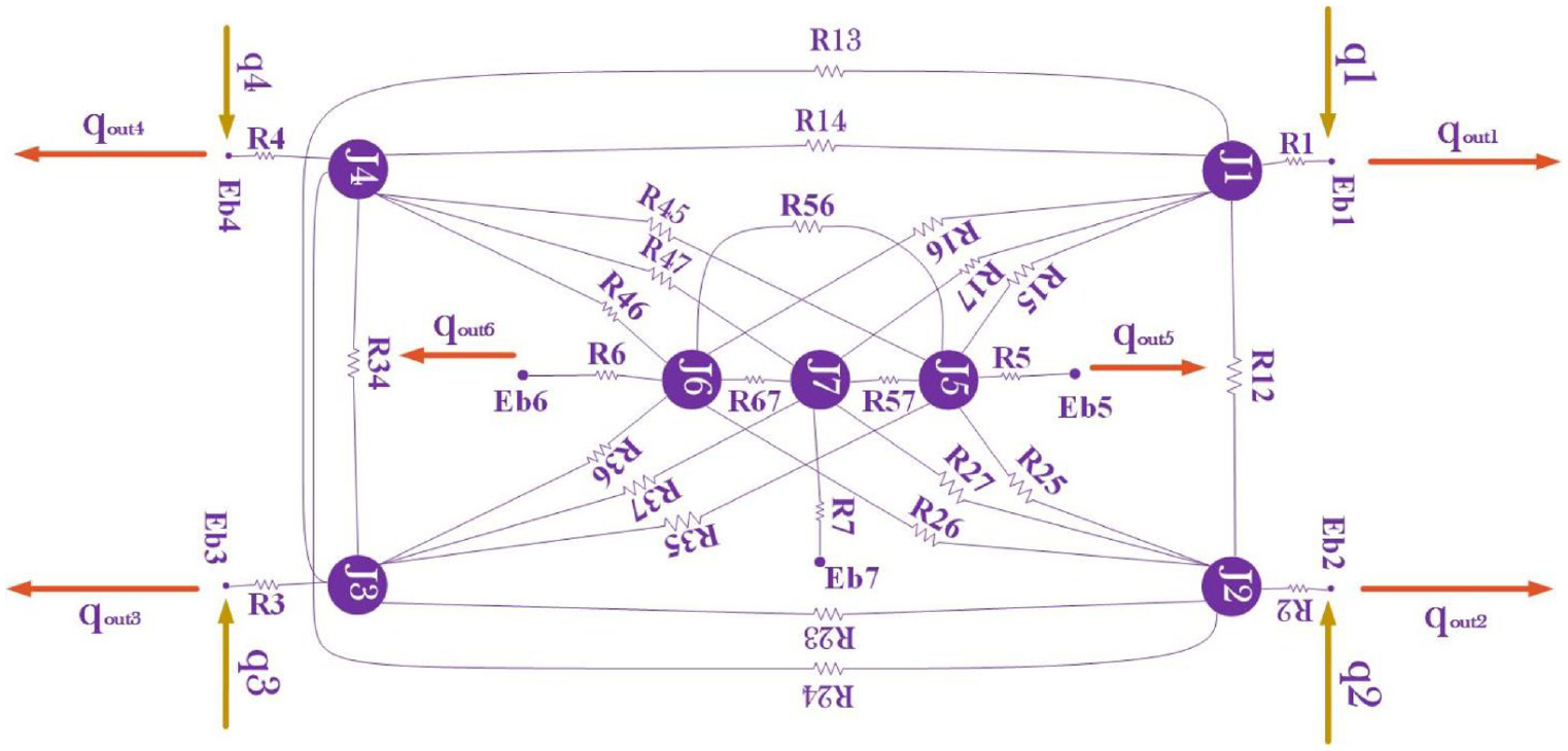
The equivalent electrical circuit for the oven’s heat transfer system.
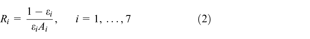
In this network, the heat flux is considered as the current. The heat transfer between nodes is radiation. For example, considering node 1, the resistance R1j represents the radiative heat transfer resistance between nodes 1 and j. The resistance R1 represents the surface radiative resistance of surface 1 (Bergman et al., 2018). In each node, the input currents and the output currents must be equal, so the following equation holds for each node:
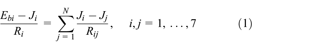
and

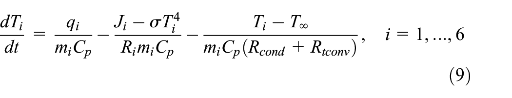
where εi is the emissivity of the surface i, Ai is the area of the surface i, and Fij is the shape factor between the surfaces i and j. The energy balance in each plate can be express by the following equation:
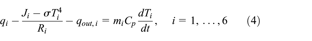
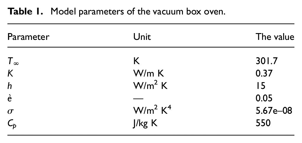
where σ is the Stefan–Boltzmann constant, Ti is the temperature of the surface i, mi is the mass of the plate i, Cp is the heat capacity, T∞ is the ambient temperature, Rcond is the conduction thermal resistance of the insulators, and Rt, conv is the convection thermal resistance.
Also, in this equation, qi is the exerted heat flux from heaters to the surface i. The exerted heat flux is zero for i = 5, 6. Moreover,
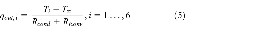
where Rt, conv is as follows:
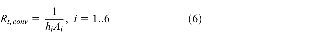
Which
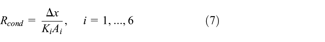
where Δx is the thickness of the insulators, and
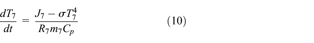
For the spherical node, the energy balance equation can be written as:
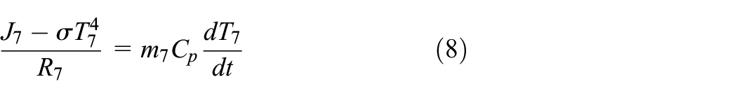
By arranging the equations (4) and (8), we have:
By expanding equation (1), the vector [Ji] can be written as follows:
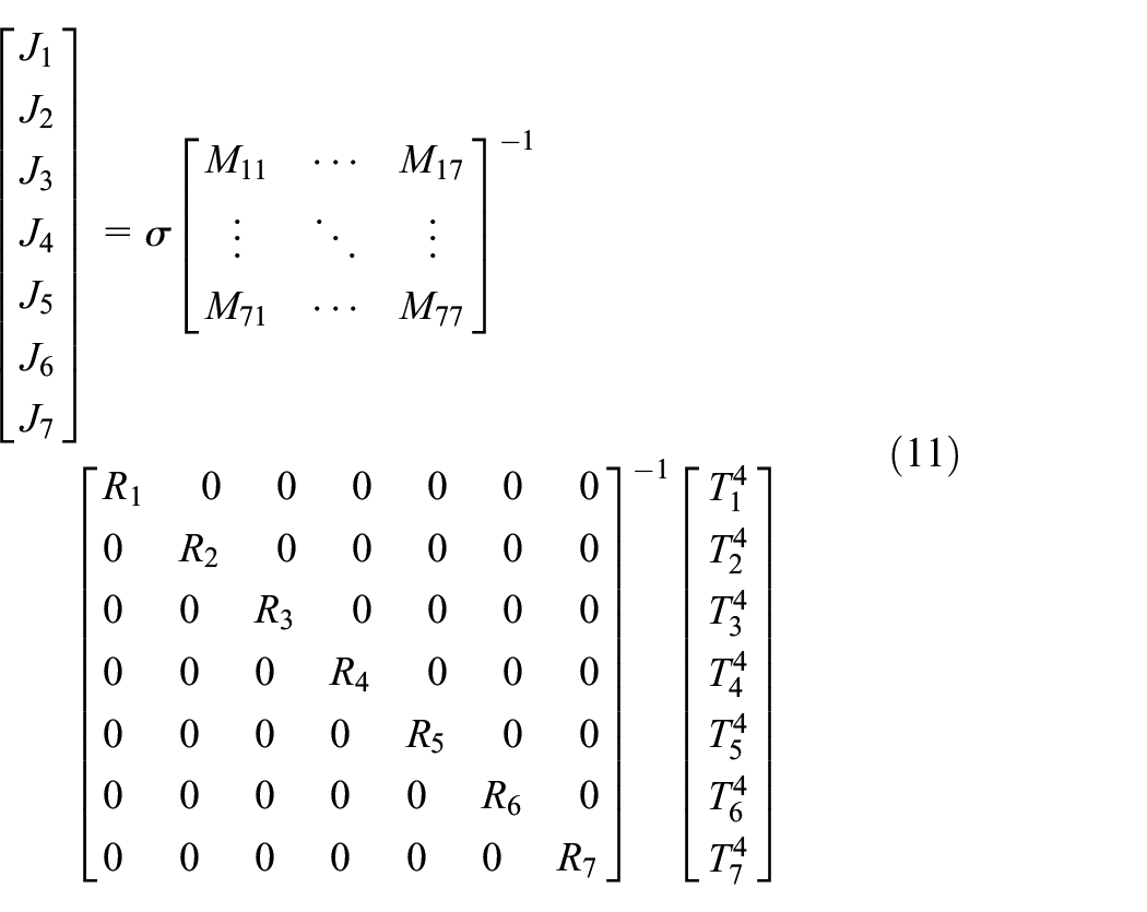
where the main diagonal elements of the matrix M are as follows:
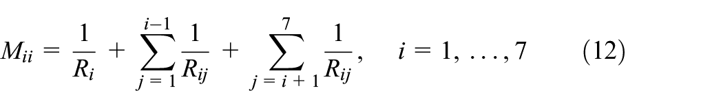
And other elements are as follows:
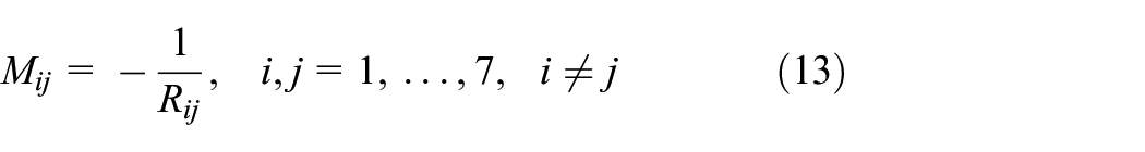
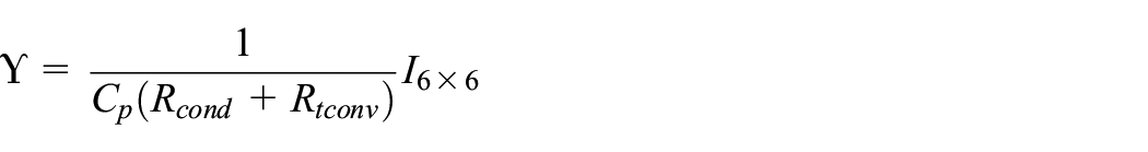
By combining the equations (9)–(11), the state-space model of the system is as follows:
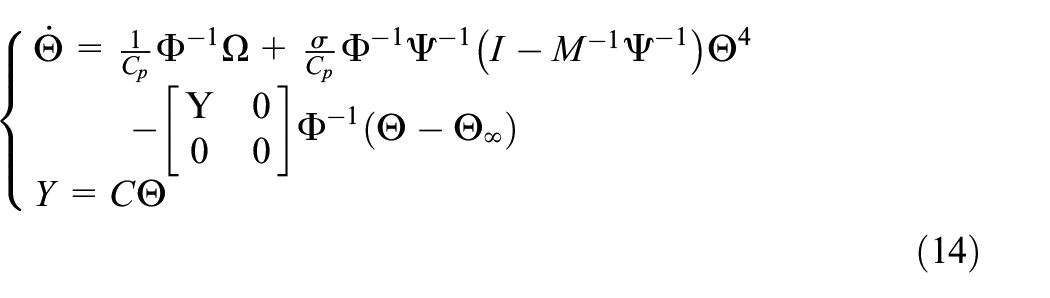
where


To obtain the elements of the matrix [Mij], the shape factors should be calculated. For parallel plates (Figure 3(a)), the shape factor can be calculated using equation (15) (Bergman et al., 2018):
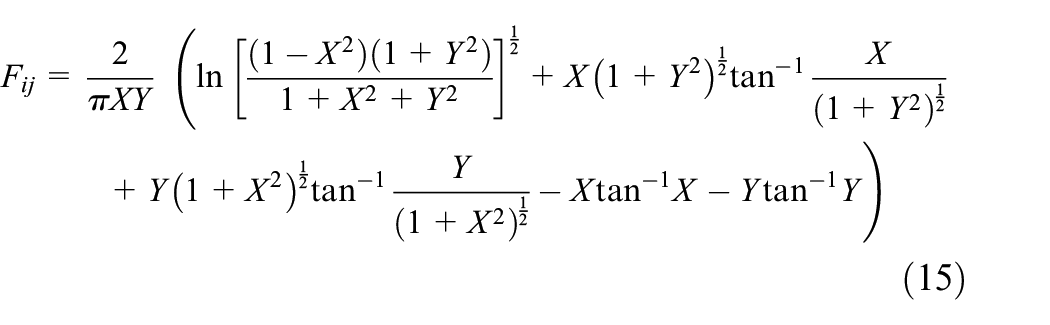
where
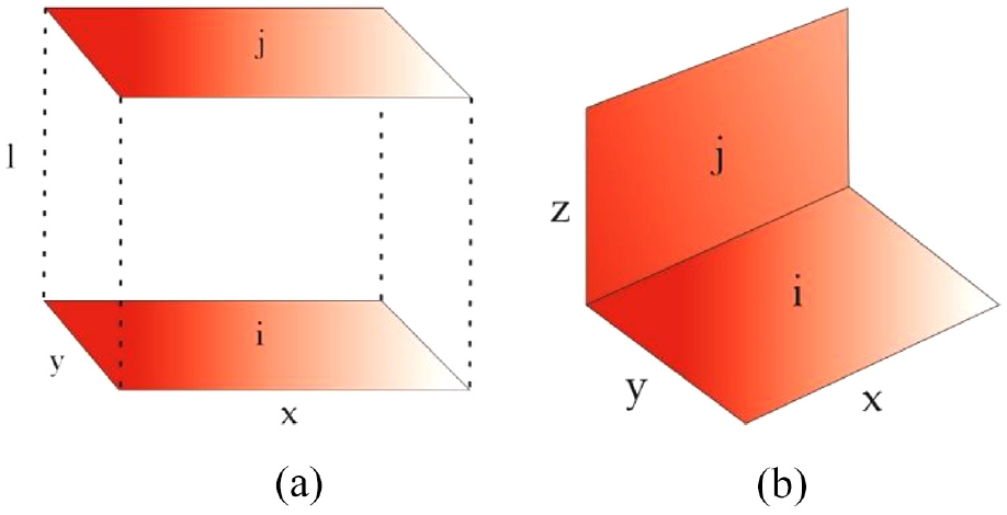
The geometry of the (a) parallel and (b) orthogonal plates for calculating shape factors. x, y, and z are the dimensions of the plates;l is the distance between the two plates, and i, j are the plate numbers.
For orthogonal plates (Figure 3(b)), the shape factor can be calculated from equation (16) (Bergman et al., 2018):
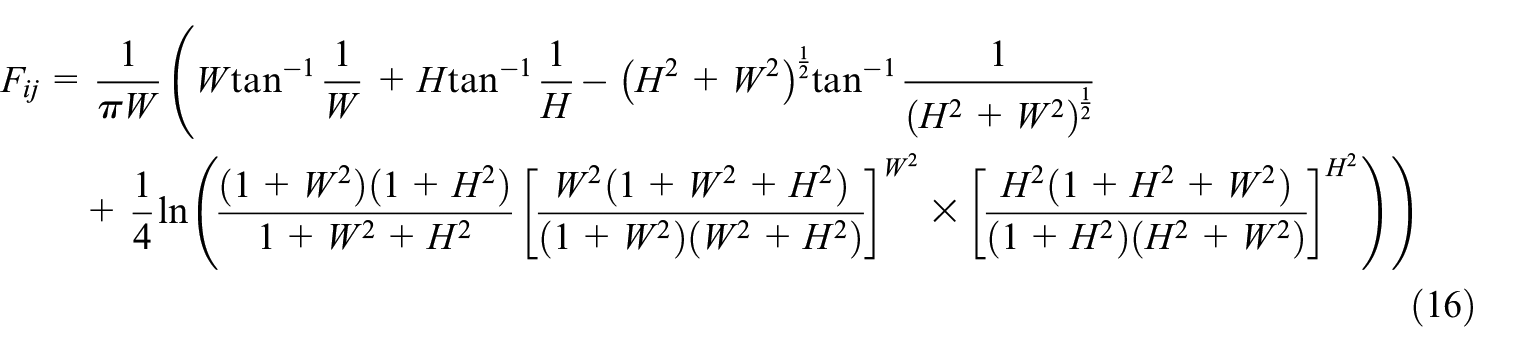
where
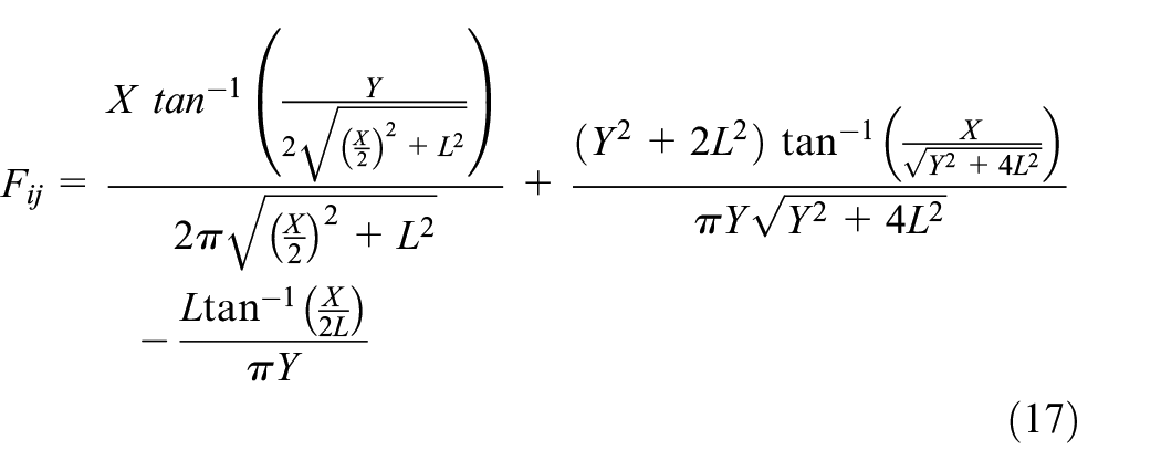
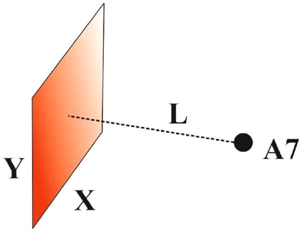
The geometry of a plate and a point.
As can be seen in Figure 4, X, Y, and L are the length of the plate, the width of the plate, and the distance between the plate and the point A7. Although the shape factors may change if a load is placed in the furnace, this uncertainty can be compensated by the controller. Hence, presenting a robust controller is essential.
Experimental setup
To verify the developed mathematical model, a vacuum oven is considered (Figure 5). This oven has about 40 L volume. The structure of this vacuum oven is similar to Figure 1. The inner space of the oven is vacuumed by a vacuum pump from a KF16 vacuum port, and then heated from four sides by four heater elements. The temperature is measured by a PT100 thermocouple. The accuracy of these sensors is one-tenth of a degree.
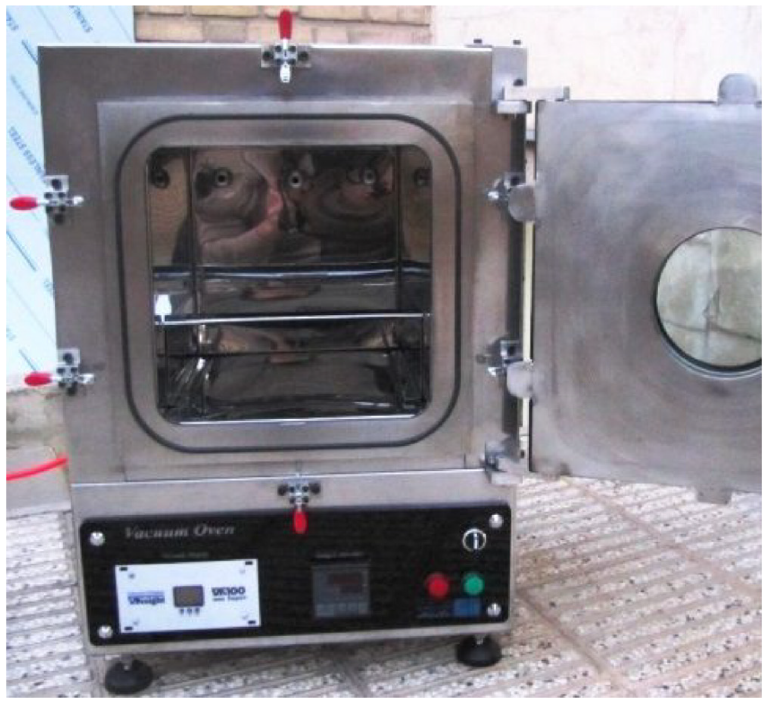
The experimental setup: a vacuum box oven.
The parameters of the model and their values for the oven are presented in Table 1. The parameters
Model parameters of the vacuum box oven.
The insulation materials used in this oven are mineral wool and ceramic board. The temperature signal is received from a PT100 sensor by a MAX 31865 module converted into understandable data for the Arduino board.
Figure 6 shows the temperate of the vacuum oven obtained from the mathematical model and the experimental setup for the same input. The experimental data are got each 30 seconds. This figure shows the good agreement between the developed model result and the experimental result.
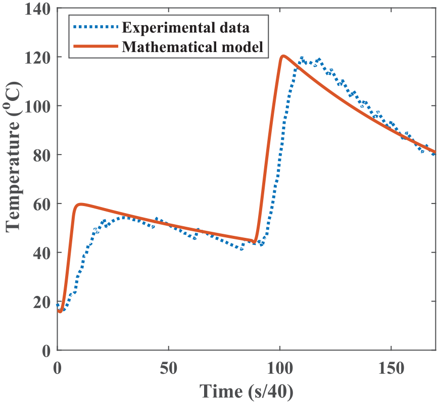
Validation of the mathematical model by experimental data.
Controller design
Control of nonlinear systems is one of the most important topics in control systems which are widely considered. The heat transfer model in a vacuum environment is one of these systems which is nonlinear. To overcome this issue, one of the most robust and popular methods is fuzzy control. A fuzzy system consists of four parts: the knowledge base, the fuzzifier, the fuzzy inference engine, and the defuzzifier. The inputs are error and derivative of the error, and its output is the heat flux. The knowledge base of the Mamdani fuzzy system is as follow:
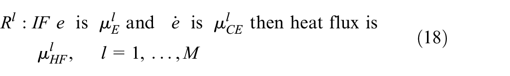
where
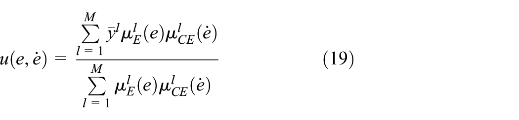
In the proposed fuzzy controller, the singleton membership function is used as the fuzzifier, and the weighted average as the defuzzifier. The inference engine is the product inference engine (Wang, 1996), where its output (control input), by using the singleton fuzzifier and weighted average defuzzifier, is as follows:
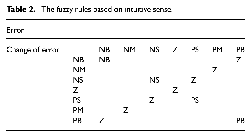
The closed-loop system with fuzzy controller is shown in Figure 7. The proposed controller acts based on the error and its derivative (change of error). However, it is different from a PD controller because in a PD controller the error and its derivative are multiplied by constant coefficients. Moreover, the proposed controller is different from a fuzzy-PD controller with adjustable gains. The symmetrical triangular membership functions are shown in Figure 8. The primary rules based on the intuitive sense are in Table 2.
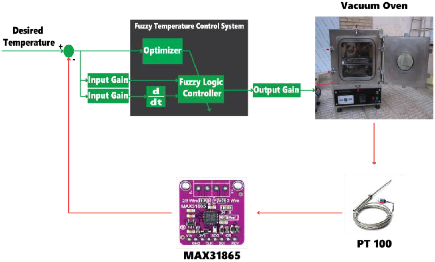
The experimental closed-loop system.
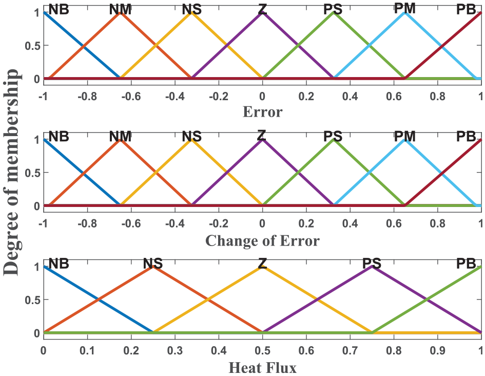
The inputs and output symmetrical membership functions.
The fuzzy rules based on intuitive sense.
The error is the difference between the desired temperature and the system temperature (system output). So, the steady-state error is this value when the system goes to its steady state. This value is measured after settling time.
First, the error and its derivative are multiplied by the input gains, and then are converted into understandable data for the fuzzy controller by using the singleton fuzzifier. The inference process is done by the product inference engine. Then, the fuzzy output signal is generated and defuzzified using the weighted average defuzzifier. Finally, the output signal is multiplied by the output gain and applied to the system.
Membership functions can be triangular, Gaussian, trapezoidal, and so on. The triangular and trapezoidal membership functions are more suitable for electrical systems because these types of membership functions are first-order mathematical functions with lower computational costs (Figure 8). In Zangeneh et al.’s study (2020), it is stated that in more than 90% of online electrical systems applications, these two types of membership functions are used. However, using non-triangular and non-trapezoidal types may lead to a more accurate response.
As shown in Figure 8, the inputs are in the interval [–1,1] and the output is in the interval [0,1]. To adjust the inputs entered to the system and the output of the fuzzy controller, two gains for inputs and a gain for output are considered (Figure 7). It causes that the controller can be adjusted for different systems by adjusting only inputs and output gains.
The behavior of the system and the control input, using symmetrical membership functions (Figure 8) and the intuitive rule base (Table 2), are shown in Figure 9. As shown in this figure, the behavior of the controller is not suitable, so, optimization is essential. The controller creates piecewise linear sections in the input. In other words, the control input does not have an acceptable smoothness. Therefore, our knowledge about the system is poor that optimization with metaheuristic algorithms can compensate this defect.
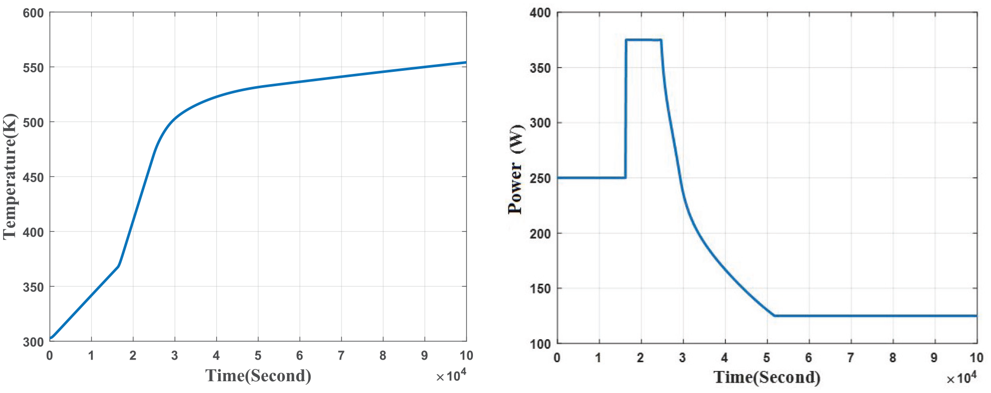
The behavior of the close-loop system and control input.
Fuzzy membership functions, rules, input and output gains are optimized with four metaheuristic algorithms, that is, GA, HS, COA, and WCA.
There are different types of metaheuristic algorithms for optimization. They can be divided into four main groups (Nazari et al., 2022); evolutionary algorithms such as GA, swarm-based algorithms such as COA, human-based algorithms such as HS algorithm, and physics-based algorithms such as WCA. In this article, one metaheuristic algorithm was selected from each group to compare them in optimization of temperature fuzzy controller.
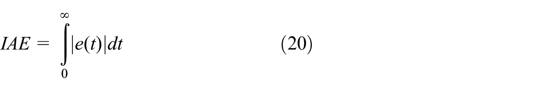
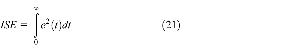
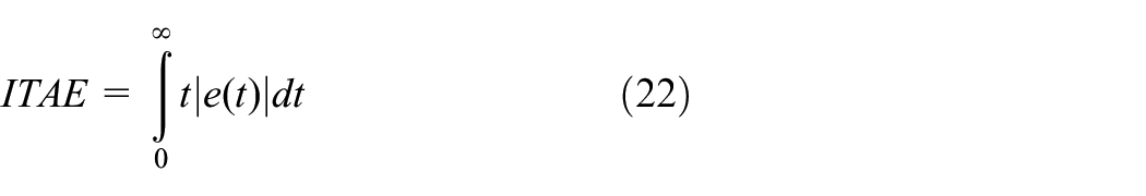
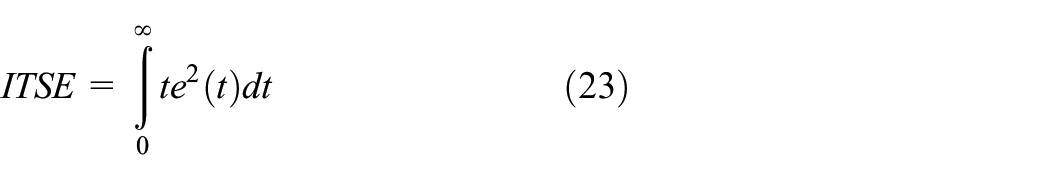
Four criteria (cost functions) of integral of square error (ISE), integral of time square error (ITSE), integral of absolute error (IAE), and integral of time absolute error (ITAE) are being used as the cost functions to optimize the fuzzy system:
The completeness and consistency of the fuzzy membership functions are regarded as constrains of the optimization problems.
In the presented fuzzy table, every tile can be placed by six rules in output and during the optimization process these tiles are placed by rules to reach the best performance.
GA
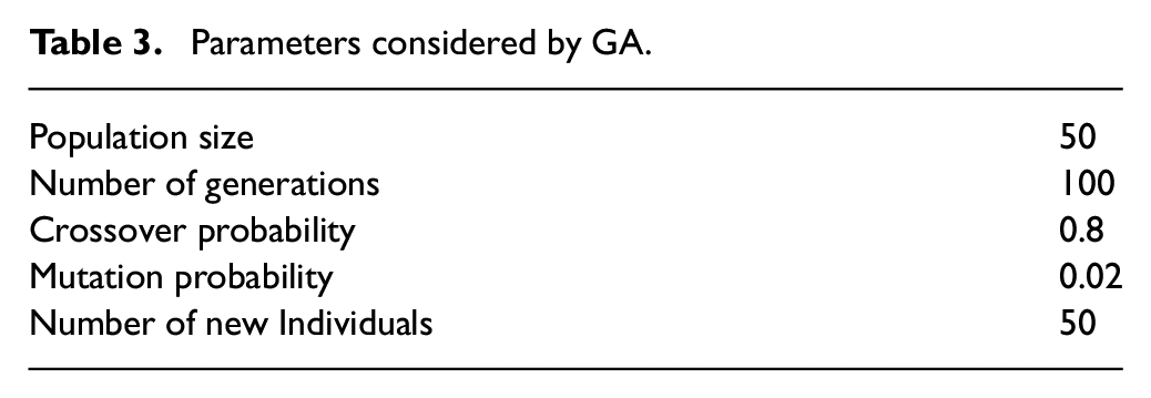
GA is a kind of metaheuristic algorithm which is inspired by natural evolution theory of Charles Darwin’s (Deepa and Sivanandam, 2008). It uses evolutionary biology techniques such as inheritance, mutation biology, and Darwin’s principles of choice to find the optimal formula for predicting or matching a pattern. According to the law of natural selection, those species that have the best characteristic will continue to reproduce and survive, and those that do not have these characteristics will disappear and become extinct during the time. To find the best answer to an optimization problem, the two main parameters of the GA, which are mutation and crossover, are used. In different problems, these processes for finding an optimum answer are happening. The flowchart of the GA is shown in Figure 10. The GA parameters are shown in Table 3.
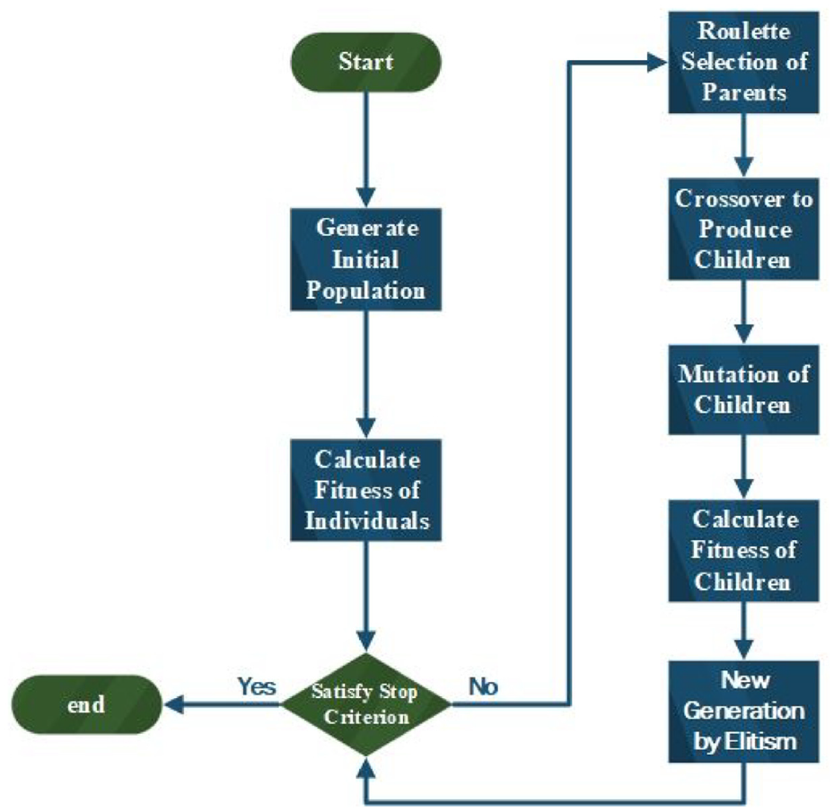
Genetic algorithm flowchart.
Parameters considered by GA.
HS
HS algorithm is a human-based algorithm inspired from harmony in music. This procedure is inspired by the emphasizing of the musician’s improvisation of harmony. In the music world, a composer or songwriter tries to compose a harmony with different amalgamation of the melodies and music pitches stored in their memory and they try to make a perfect harmony (Gao et al., 2015). This process can be used in engineering problems to enhance answers.
First, a harmony memory (HM) is effectuated to optimize the problem and then a new solution is expedient. For the N-dimension problem, the HM can be written as follows:
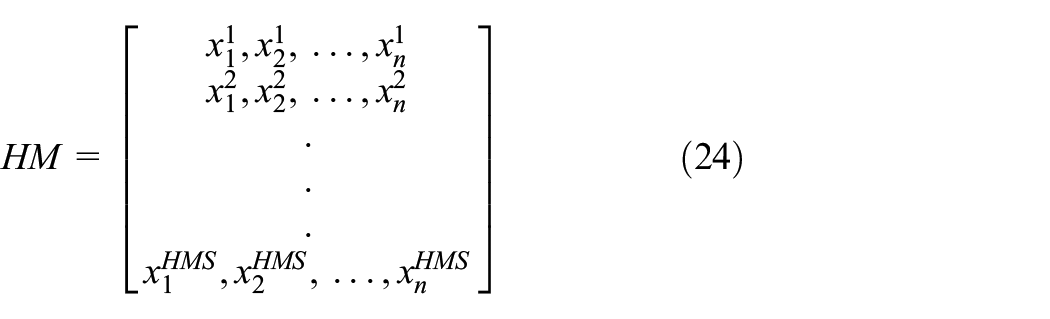
where

If

where Delta is as follow:

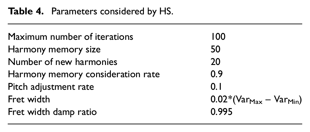
The parameter FW is determined by the upper and lower bounds of the problem. Clearly, the improvisation in HS is alike to the production of offspring in GA with the mutation and crossover operations. The difference is the GA uses only one mutation or two simple crossovers to create new chromosomes, while the creation of new solutions in the HS procedure is to advantage all the HM members. The HM is updated and the new solutions evaluate and the HM is merged with a new harmony. This process is continued until a termination criterion is met. The HS parameters are shown in Table 4.
Parameters considered by HS.
COA
The COA is inspired by the cuckoo’s behavior in reproduction (Rajabioun, 2011). In the wild, cuckoos do not build nests and instead lay their eggs in the nests of other birds, and cuckoo eggs in these nests get a chance to hatch. The higher the chances of the eggs hatching in the nests of an area, the better that area is for cuckoos to lay eggs. In an optimization problem, an optimum answer can be found near these areas. Cuckoos lay their eggs in the same color as the eggs of the host bird so that the host bird does not recognize the cuckoo’s eggs. Cuckoos try to protect the eggs. And also, the cuckoos try to migrate to safer places to protect the eggs and the survival of the offspring. Initially, to solve the optimization problem, like other evolutionary algorithms, a population of cuckoos is formed, each of which has a place in the problem space. Also, each cuckoo in the initial population lays several eggs within a radius of the environment. These eggs will become chicks and finally become mature birds. These cuckoos formed a society in which each of them has a habitat area to live in. The best habitats of all societies will be the target of all cuckoos. Then cuckoos try to immigrate to the best habitat for laying eggs.
In an optimization problem, a habitat is an N-dimensional array.

The profitability of the current habitat can be evaluated by the following profit function:

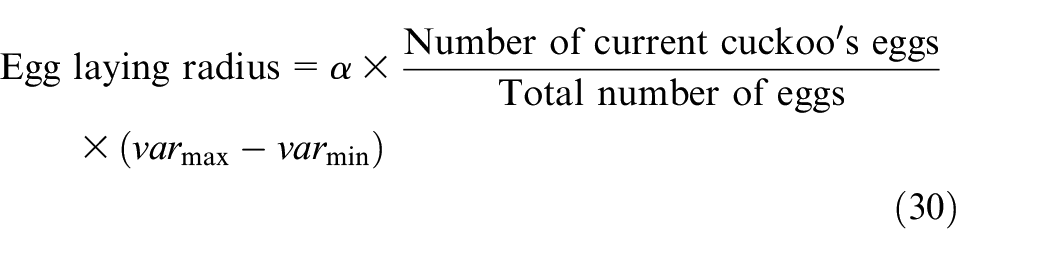
A habitat matrix in size of Npop*NVar will be prepared for starting an optimization algorithm, then for each habitat a random number of eggs will be allocated (Akbarzadeh and Shadkam, 2015). The egg-laying radius obtained from the following equation:
And finally, the migration formula is:

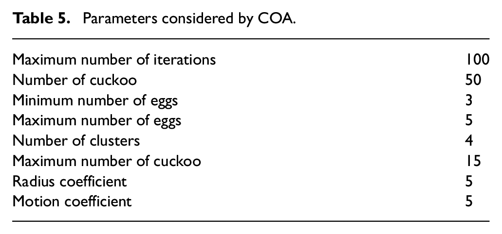
The COA parameters are shown in Table 5.
Parameters considered by COA.
WCA
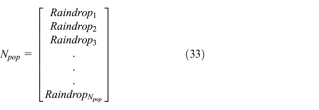
The WCA is one of the metaheuristic algorithms inspired by the water cycle process in nature. It is based on how streams and rivers create and flow to the sea (Eskandar et al., 2012). The main processes in the water cycle that is used in this algorithm are raining, surface movement of streams and rivers toward the sea, evaporation and condensation. Initially, a population of raindrops is formed in a form of an NVar array as follows:

where Npop is:
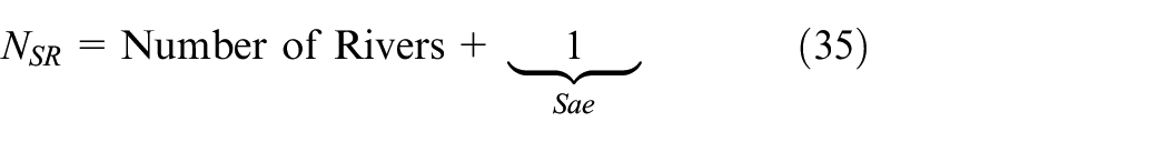
The number of streams calculated as follows:

where NSR is:
Due to the intensity of the current in the sea and rivers, each of the streams is allocated to rivers and seas. The movement of streams toward the sea is obtained from the following relation:

The movement of streams toward the rivers is obtained from the following equation:

And finally, the movement of rivers toward the sea is obtained from the below equation:

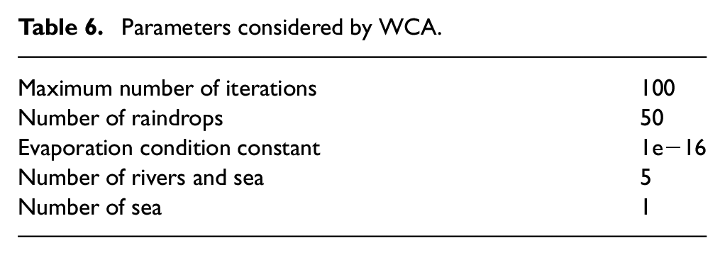
The WCA parameters are shown in Table 6.
Parameters considered by WCA.
Results and discussion
In all simulations, the desired temperature is 500°K, and the initial temperature is 303°K. The maximum heat flux is limit to 0–400 W, which is a constraint in the optimization problem.
Using the GA
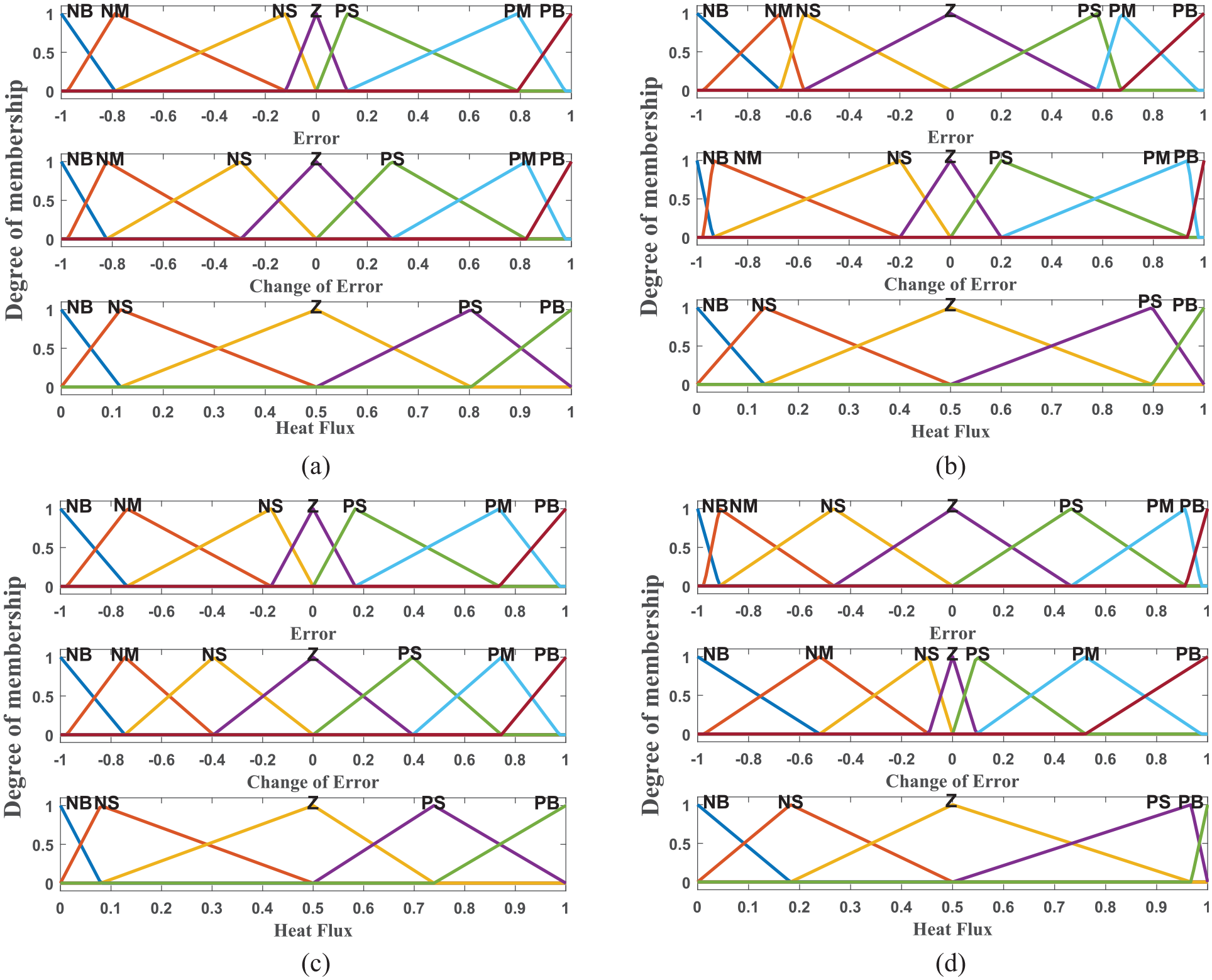
The fuzzy membership functions obtained from the four criteria using GA are shown in Figure 11.
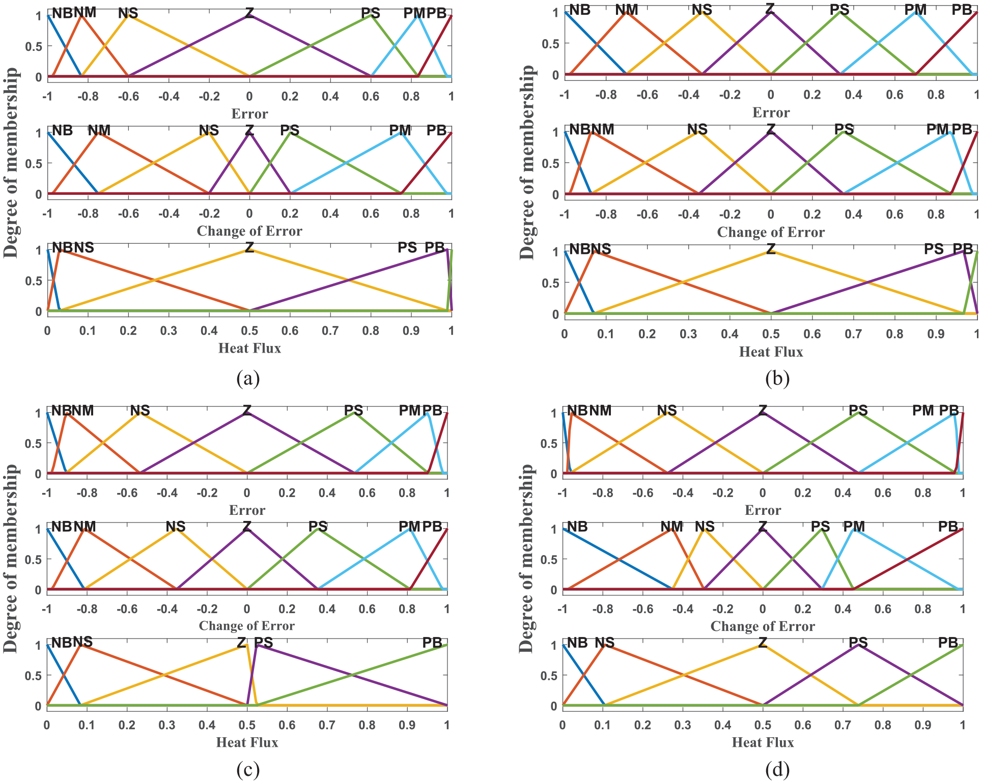
Input and output fuzzy membership functions using GA with (a) ISE, (b) ITAE, (c) ITSE, and (d) IAE.
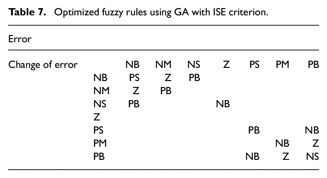
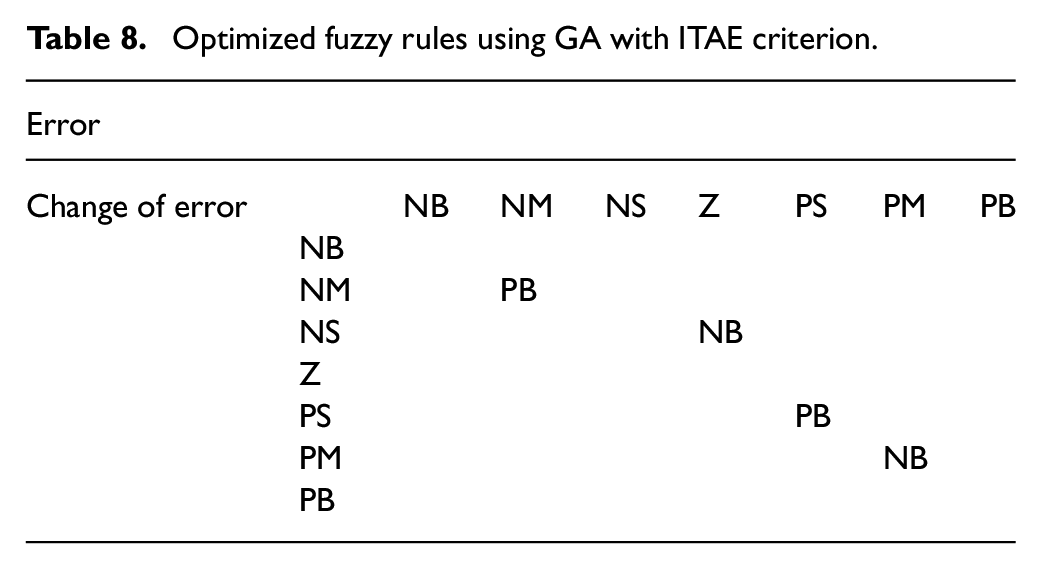
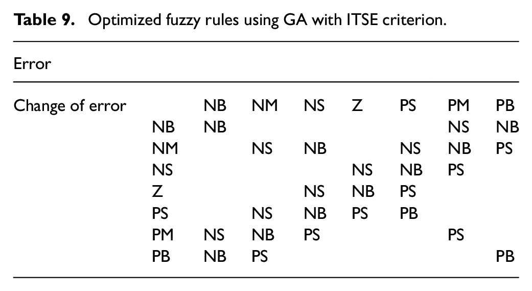
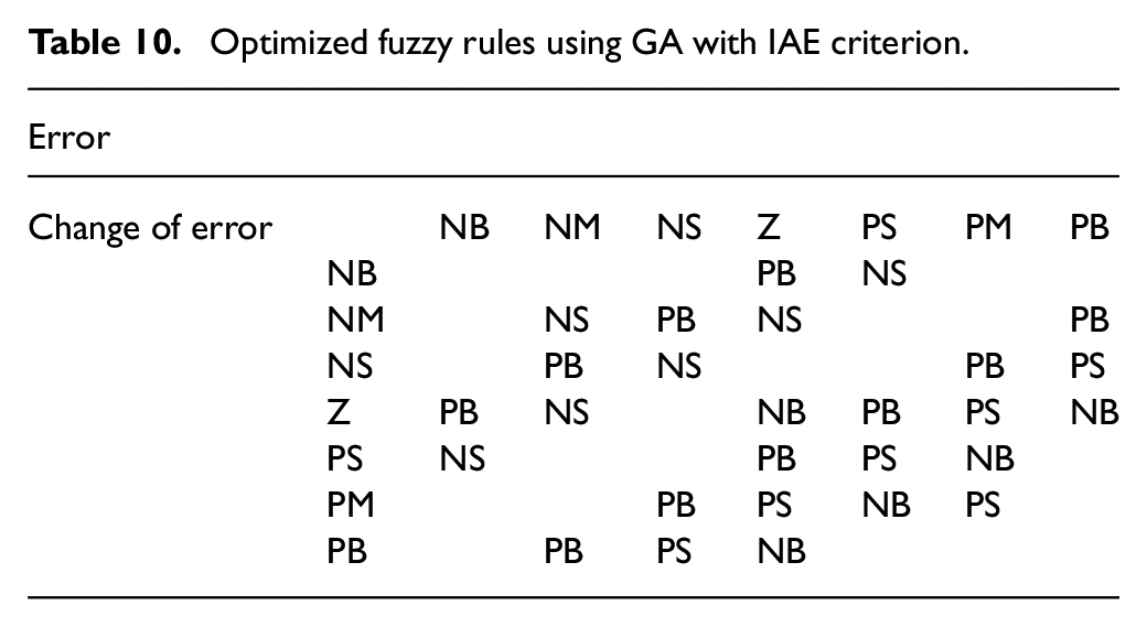
The optimized fuzzy rules using GA are shown in Tables 7–10. As shown in these tables and Figure 11, different criteria made different rule bases and membership functions.
Optimized fuzzy rules using GA with ISE criterion.
Optimized fuzzy rules using GA with ITAE criterion.
Optimized fuzzy rules using GA with ITSE criterion.
Optimized fuzzy rules using GA with IAE criterion.
The optimized input and output gains using GA are shown in Table 11.
Inputs and output gains using GA.
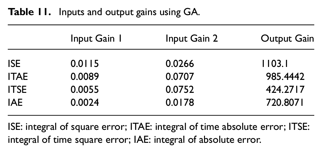
ISE: integral of square error; ITAE: integral of time absolute error; ITSE: integral of time square error; IAE: integral of absolute error.
The behavior of the system and the performance of the GA-Fuzzy control are presented in Figure 12. As shown in Figure 12(a), all responses have a steady-state error, and using the ITAE criterion has made the minimum steady-state error, but its overshoot is high. The steady-state error is the difference between the desired temperature and system output at time
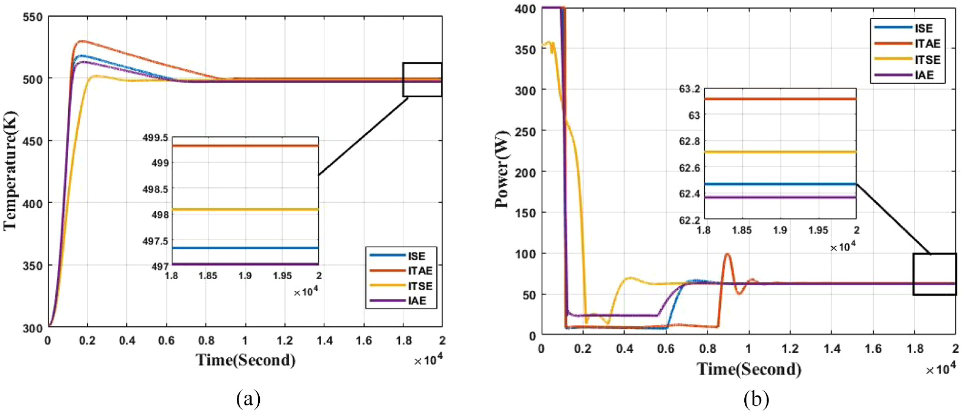
(a) The behavior of the closed-loop system and (b) fuzzy control input using GA.
Using the HS
The membership functions obtained from the f criteria using HS algorithm are in Figure 13.
Input and output fuzzy membership functions using HS with (a) ISE, (b) ITAE, (c) ITSE, and (d) IAE.
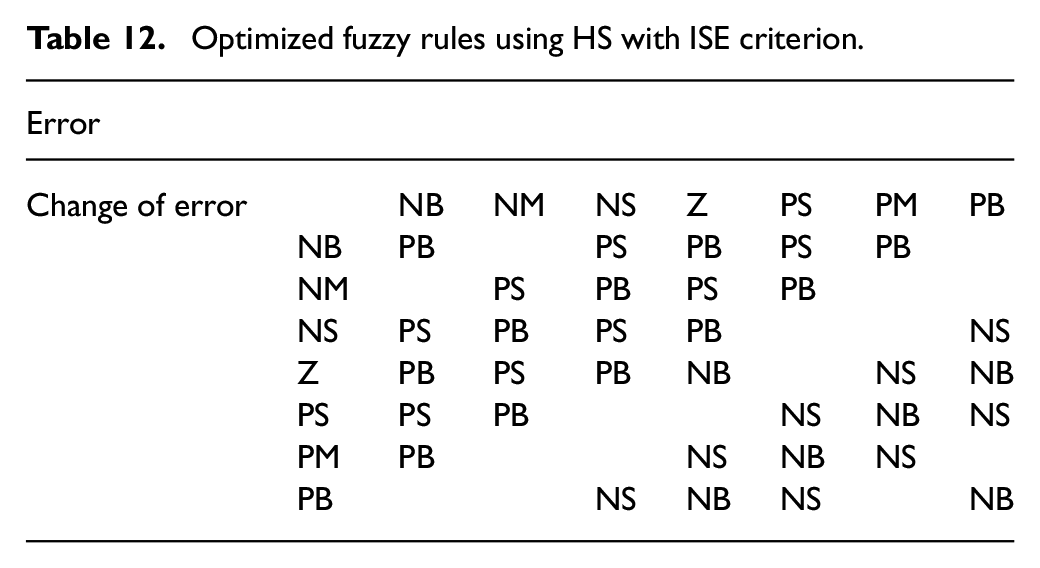
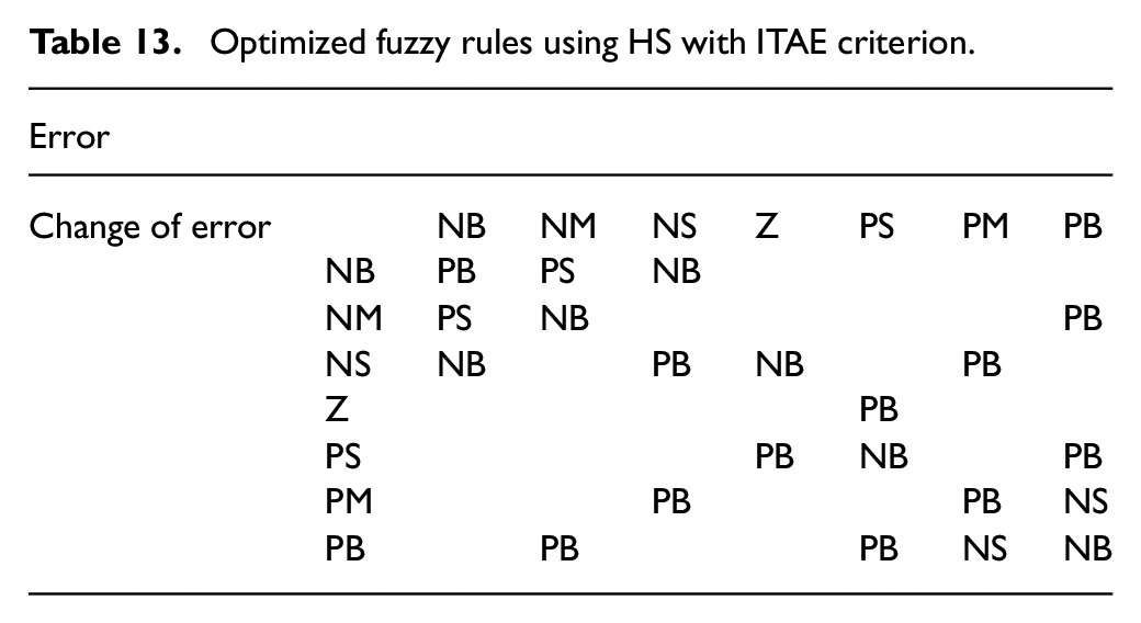
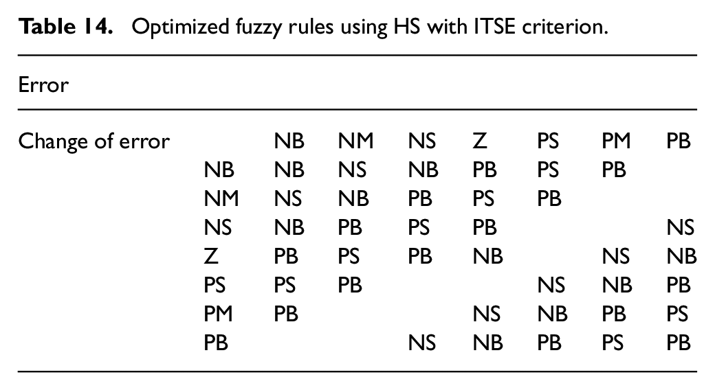
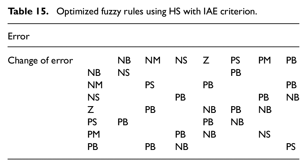
The optimized fuzzy rules are shown in Tables 12–15.
Optimized fuzzy rules using HS with ISE criterion.
Optimized fuzzy rules using HS with ITAE criterion.
Optimized fuzzy rules using HS with ITSE criterion.
Optimized fuzzy rules using HS with IAE criterion.
The inputs and output gains are shown in Table 16.
Inputs and output gains using HS.
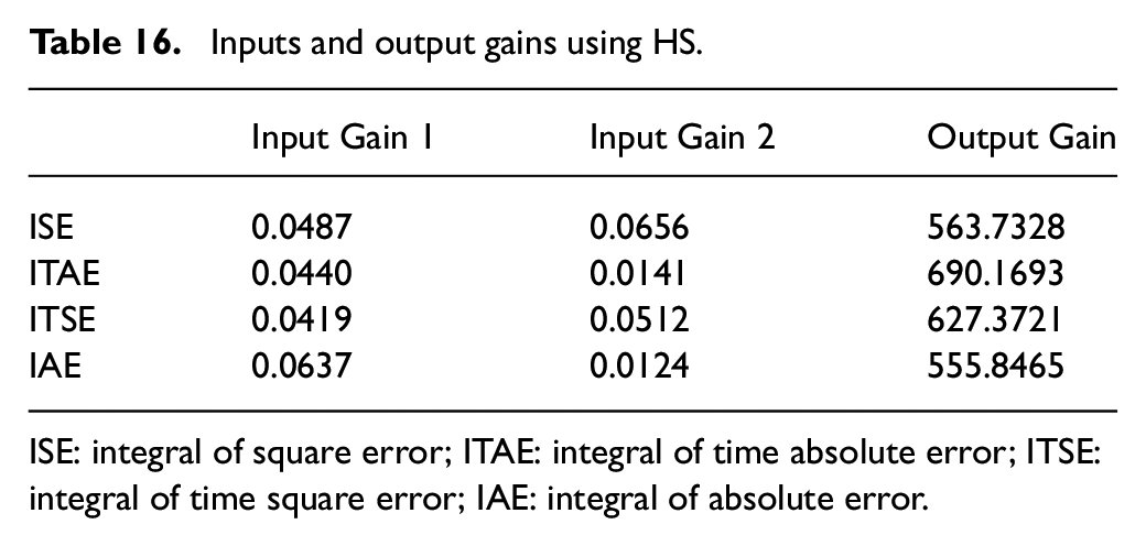
ISE: integral of square error; ITAE: integral of time absolute error; ITSE: integral of time square error; IAE: integral of absolute error.
The behavior of the system and the fuzzy control input using the HS algorithm are presented in Figure 14. The minimum steady-state error is obtained by using the ITAE criterion. However, in the sense of both steady-state error and overshoot, using ISE and ITSE criteria is better. ITSE criterion gets lower rise time than ISE criterion. As shown in Figure 14(b), the implemented inputs using ISE and ITSE have lower amplitudes at the beginning, which makes lower overshoot.
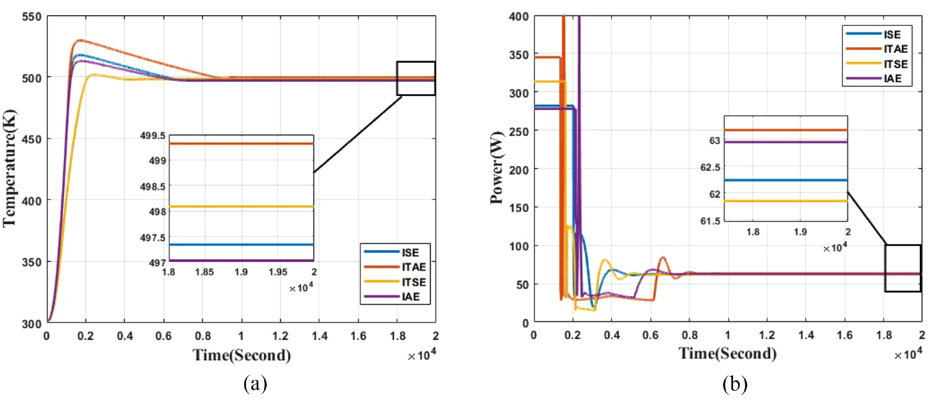
(a) The behavior of the closed-loop system and (b) the fuzzy control input using HS algorithm.
Using the COA
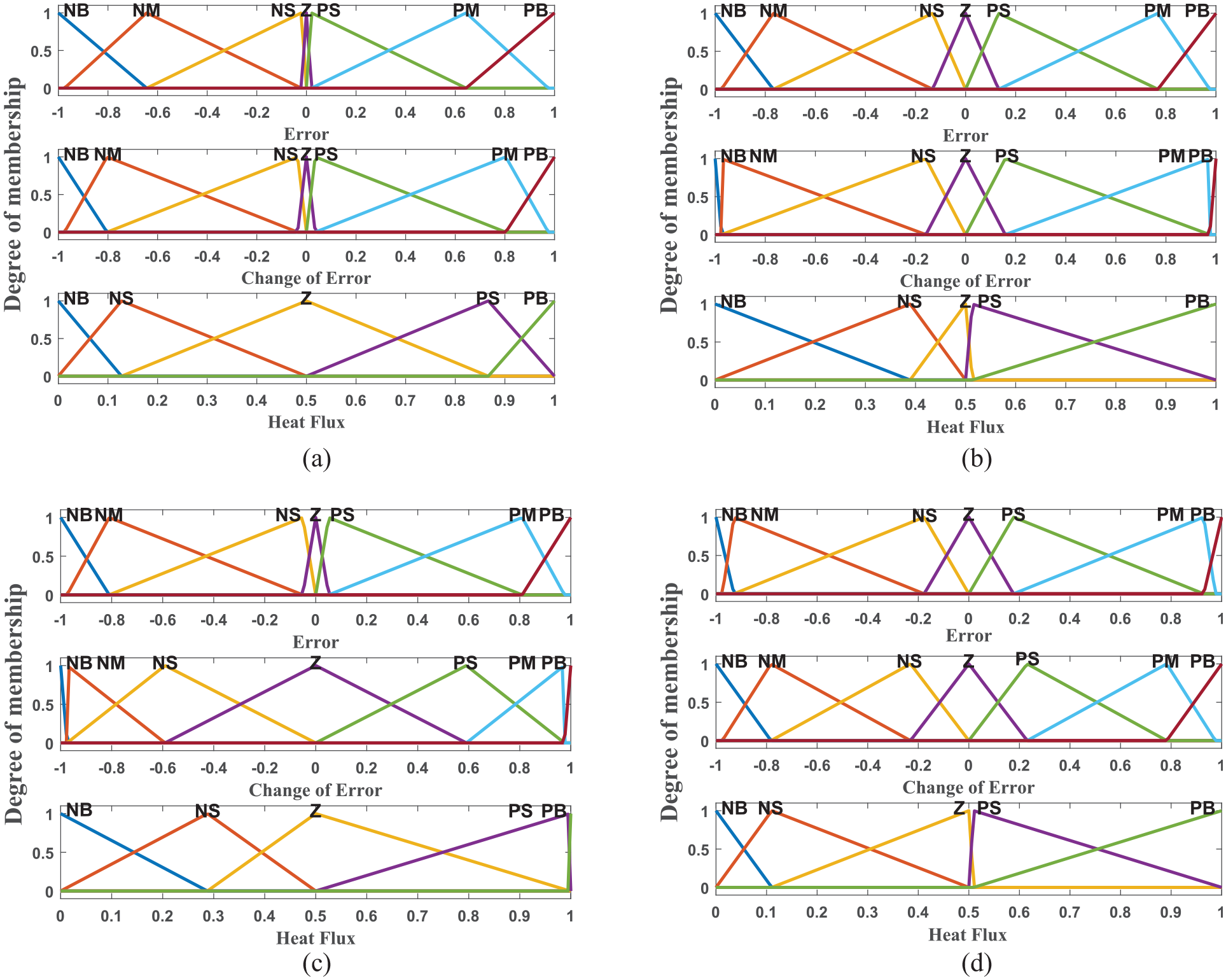
The fuzzy membership functions obtained from two criteria, that is ISE and ITSE, are shown in Figure 15. There are not any stable responses with the two others criteria.
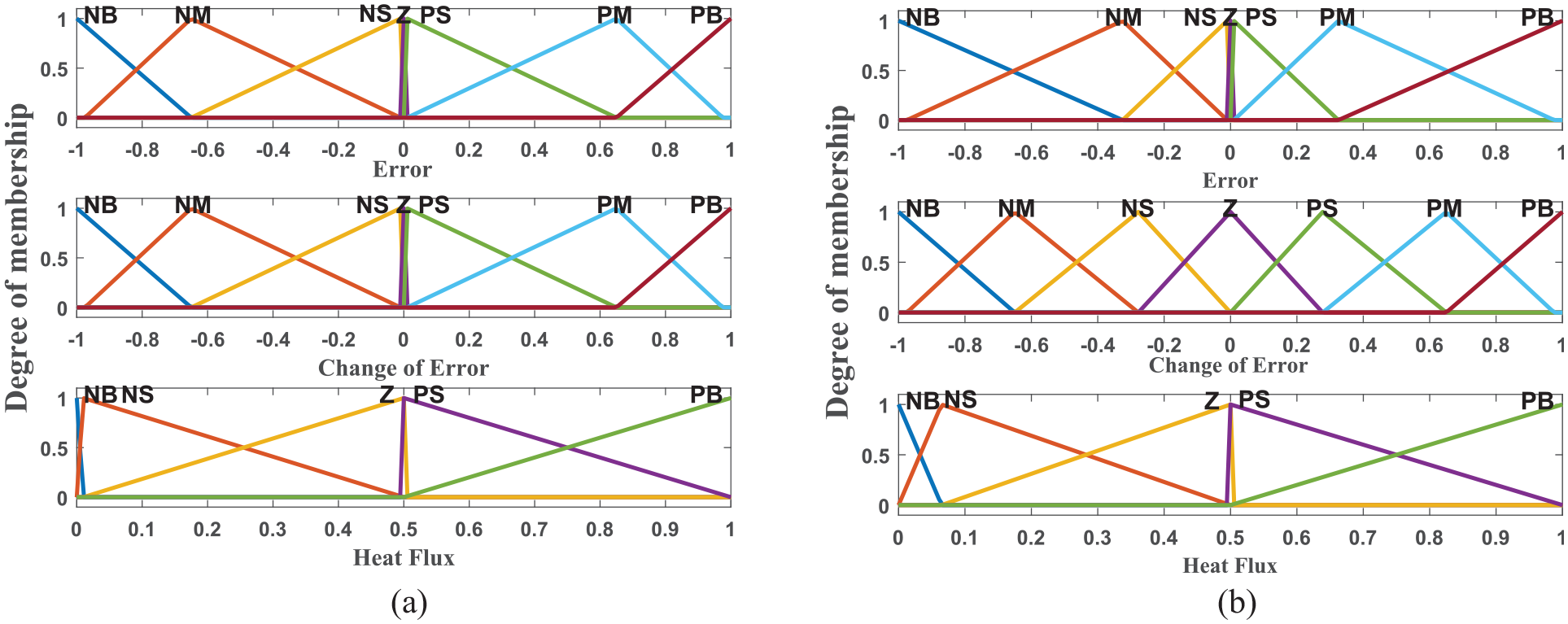
Input and output fuzzy membership functions using COA with (a) ISE and (b) ITSE.
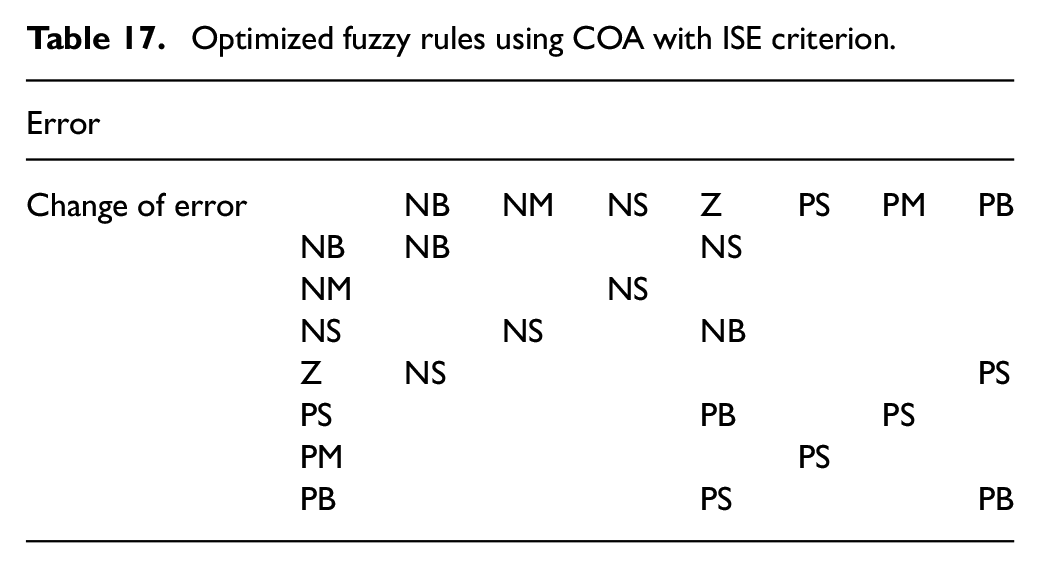
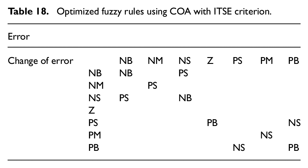
The optimized fuzzy rules are shown in Tables 17 and 18.
Optimized fuzzy rules using COA with ISE criterion.
Optimized fuzzy rules using COA with ITSE criterion.
The inputs and output gains are shown in Table 19.
Inputs and output gains using COA.
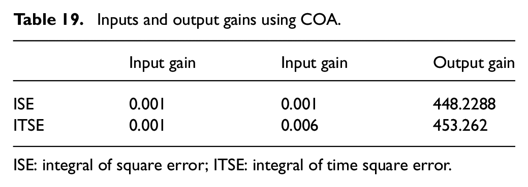
ISE: integral of square error; ITSE: integral of time square error.
The behavior of the system and the fuzzy control input using COA are presented in Figure 16. In comparison, the ISE criterion is better. Totally, their responses are not suitable. Moreover, as shown in Figure 16(b), the control inputs are fluctuating.
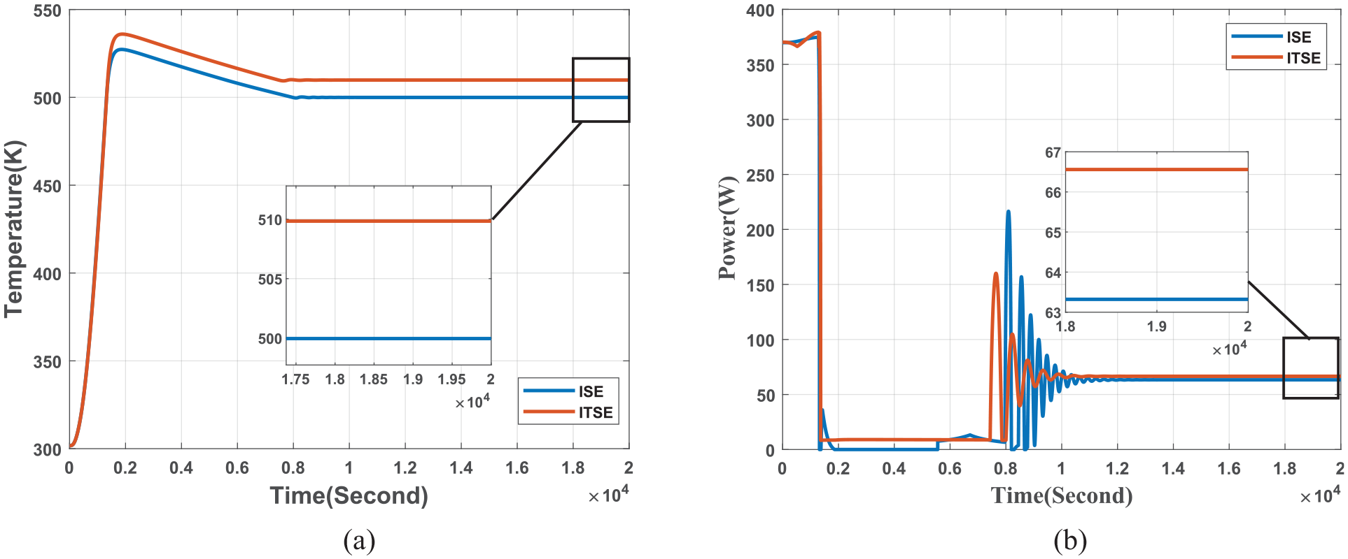
(a) The behavior of the closed-loop system and (b) the fuzzy control input using COA.
The input gains are very small which cause to place error and change of error around zero. Moreover, the membership function around zero (“Z”) for error and change of error is very concentrated. Hence, the output of the fuzzy inference engine (control input) changes with a slight change in the value of error (or change of error). This causes fluctuation in the control input. Since the “Z” membership function for change of error in the ITSE criterion is not concentrated, the control input in this criterion is less fluctuating.
Using the WCA
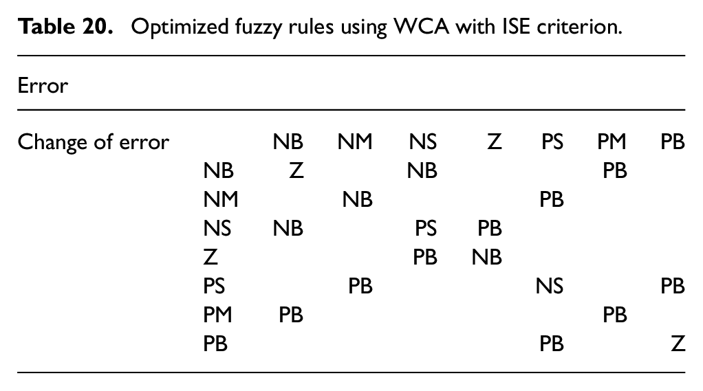
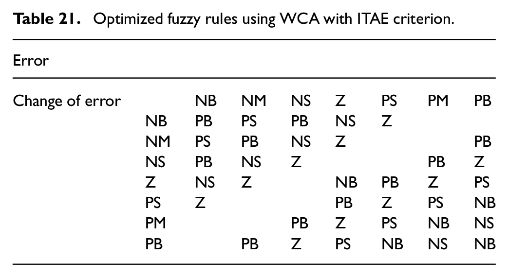
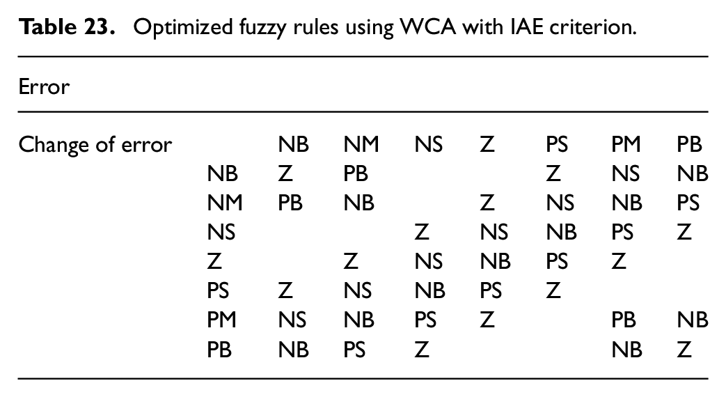
The fuzzy membership functions obtained from the four criteria using WCA are shown in Figure 17. Moreover, the optimized fuzzy rules are shown in Tables 20–23.
Input and output fuzzy membership functions using WCA with (a) ISE, (b) ITAE, (c) ITSE, and (d) IAE.
Optimized fuzzy rules using WCA with ISE criterion.
Optimized fuzzy rules using WCA with ITAE criterion.
Optimized fuzzy rules using WCA with ITSE criterion.

Optimized fuzzy rules using WCA with IAE criterion.
The inputs and output gains are shown in Table 24.
Inputs and output gains using WCA.
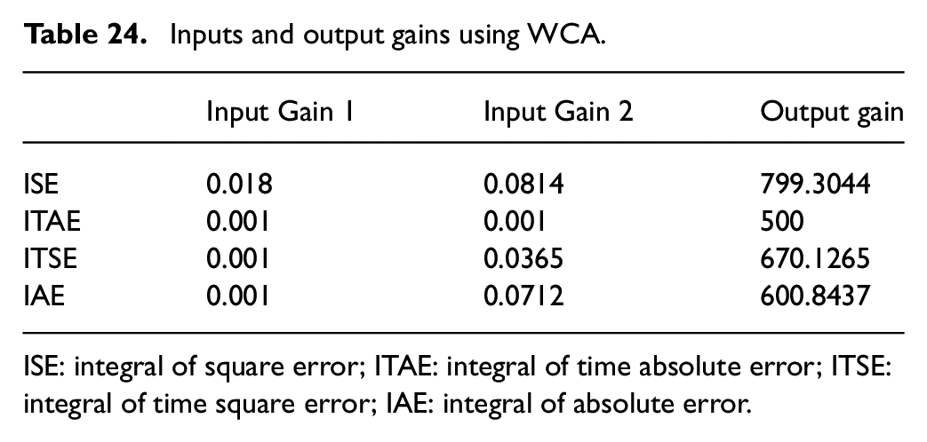
ISE: integral of square error; ITAE: integral of time absolute error; ITSE: integral of time square error; IAE: integral of absolute error.
The behavior of the system and the fuzzy control input using WCA are presented in Figure 18. In all cases, the overshoot is low. However, using ITAE makes the lowest steady-state error and overshoot. The control inputs are shown in Figure 18(b). The ITSE criterion gets lower rise time.
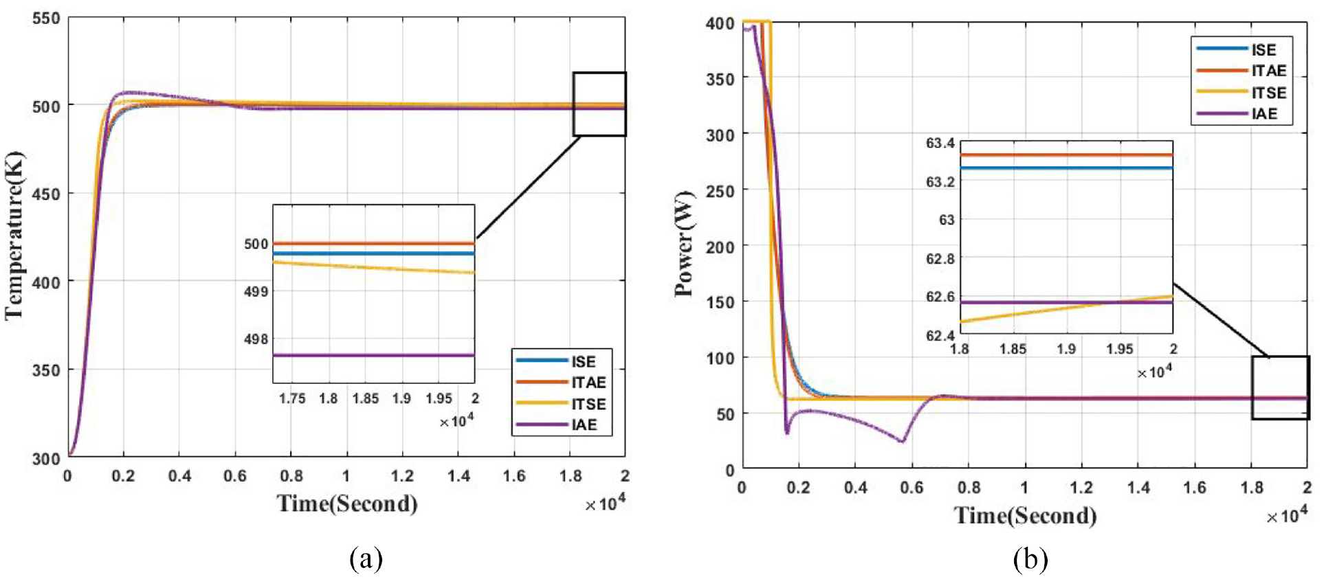
(a) The behavior of the closed-loop system and (b) the fuzzy control input WCA.
The cost function values for each optimization method are shown in Table 25.
The value of the cost functions for each optimization algorithm.
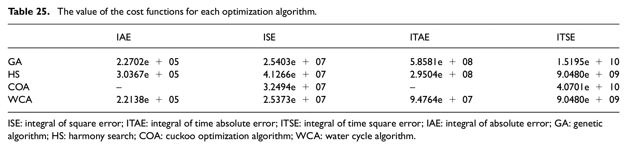
ISE: integral of square error; ITAE: integral of time absolute error; ITSE: integral of time square error; IAE: integral of absolute error; GA: genetic algorithm; HS: harmony search; COA: cuckoo optimization algorithm; WCA: water cycle algorithm.
By comparing the results, the following conclusions are obtained:
In all criteria, in 500 K, WCA had the best performance.
In ITSE, the HS algorithm and WCA had the best performance.
The COA could not optimize the controller.
The ITAE criterion got the minimum steady-state error in all cases.
Totally, using ITSE criterion got better both steady-state error and overshoot.
In all cases, the fuzzy set of the elements in the secondary diagonal is NB. Hence, in all cases, the implemented input at steady state is NB. This is because to regulate the temperature at its desired value, the inlet heat flux from heaters must be equal to output heat flux from the system. Hence, the control input at steady state is not zero. Different control inputs in different cases are related to the shape of the membership functions and inputs and output gains.
The implemented input in the steady state is almost equal in all cases.
Almost in all cases, the implemented input at the beginning is at its maximum value which is one of the advantages of the fuzzy controller in comparison with the PID controller. It can improve the response speed of the system. Although this defect can be compensated by high proportional gain in the PID controller, it causes high overshoot.
The fuzzy controller is robust against uncertainties. The differences among the controllers are in membership functions shapes, input and output gains, and rule-bases. Therefore, it can be concluded that all of them are robust with different control performances.
So, in the transient response, the ITSE criterion is better, and in the steady-state response, the ITAE criterion is the best. Because the square of error is significant in the transient response and the absolute of the error is significant in the steady-state response. Therefore, a new fuzzy controller can be a mix of them that is, a fuzzy controller optimized with ITSE criterion before the settling time, and then switch to another fuzzy controller optimized with ITAE criterion after settling time.
To evaluate the performance of the optimized controllers, the behaviors of the closed-loop system in other set-points that is, 400 K, 500 K, and 600 K are plotted (Figure 19). Since the controllers had the best performances in the ITSE criterion, the optimized controllers using this criterion are considered. As shown in Figure 19a, at 400 K and 500 K, all controllers have accepted performances except the fuzzy controller optimized with COA (Fuzzy-COA). Although the Fuzzy-WCA had the best performance in all criteria in 500 K, its performance in 600 K is not accepted. Figure 19b shows the implemented control inputs. The control input of the optimized Fuzzy-COA using ITSE criterion has fluctuations. Using ITSE criterion, Fuzzy-GA gets lower control input at each set point change and Fuzzy-WCA gets higher.
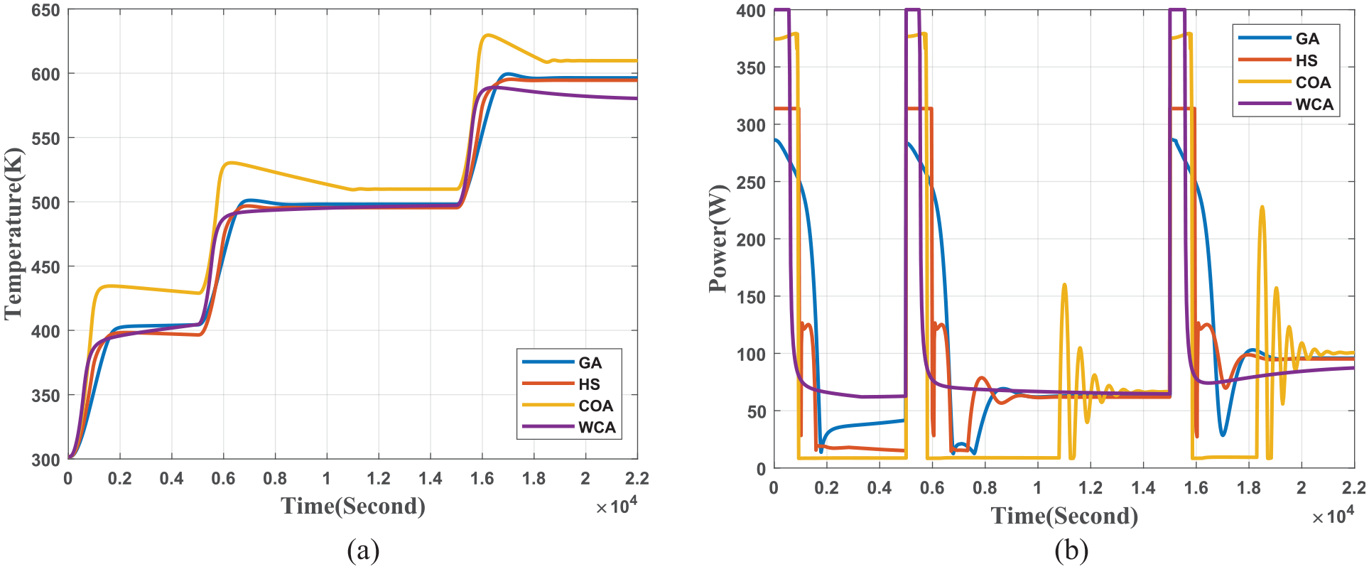
Comparing the behavior of the closed-loop system in other set-points that is, 400 K, 500 K, and 600 K using the ITSE criterion.
By attention to the control input implemented by different controllers in Figure 19(b), it is understood that the WCA-fuzzy controller gives more control input at first for all set-points. Hence, its delay time is lesser than other controllers. When the system approaches the set-points (the error is “Z” and the change of error is “PS” or “NS”), the WCA-fuzzy controller gives more heat flux at 400 K and 500 K and less control input at 600 K. It comes back to the shape of “NB” and “PB” membership functions of the output and the output gain in these controllers.
GA and HS algorithm have the best performance; the Fuzzy-GA gets the least steady-state error and Fuzzy-HS gets no overshoot. Each of them has its applications; in some applications having no overshoot is important such as drying or heat treatment processes, and in other applications having no error is important such as precise research in the laboratories.
Experimental test of the fuzzy controller
The behavior of the system using Fuzzy-GA-ITSE controller and the control input in the experimental test is shown in Figure 20. As can be seen in Figure 20a, the closed-loop system behavior is similar to the simulation results. To control the oven temperature, the voltage applied to the heater elements must be changed. On the contrary, the voltage required to operate the heater elements is 220 volts. By changing the voltage, heater elements will not operate. Therefore, the voltage required for the heater elements is applied as a pulse width modulation (PWM) signal which it works by pulsating DC current, and varying the amount of time that each pulse stays “on” to control the amount of current that flows to a device. The longer each pulse is on, the more flow to the device will be. Due to the fact that the interval between pulses is so brief, the device does not actually turn off. In other words, the device’s power source switches on and off so fast (thousands of times per second) that the device actually stays on without flickering. This is called PWM dimming (Brown, n.d.). Comparing the control input in the experimental test and the simulation results, it is observed that in the experimental test, the control signal has an oscillating behavior, which is due to the nature of the PWM operation. (Figure 20b). As shown in Figure 20b, by using the Fuzzy-GA-ITSE controller, the maximum power is exerted to the system at first; then the control input decreases to settle the temperature at desired value
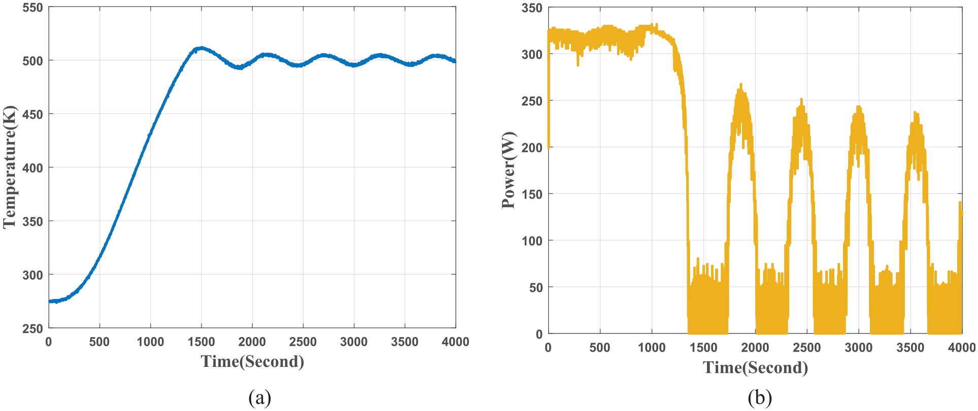
The behavior of the system and control input.
Comparison between the simulation and experimental results shows that the rise time and overshoot are close. The deviation between them may be due to the test conditions, uncertainty in real parameters and model parameters, and implementation of the Fuzzy-GA-ITSE controller using PWM. It should be noted that there is some deviation between mathematical model and the real system (Figure 6). However, the experimental test not only shows that the proposed controller is robust but also states that the developed model has accepted accuracy.
The control input in simulation and experimental results are almost similar. At first, the value of control input in simulation and experimental result is somewhat different which may be due to the difference in initial conditions (initial temperatures).
Between the time 1500s and 4000s in Figure 20(b), the closed-loop system is around the set-point (the error is “Z”). Changes in control input amplitude are due to changes from “PS” to “NS” and vice versa. Since the overlap among “NS,”“Z,” and “PS” is low, the switch among them is fast which causes changes in control input amplitude. However, as shown in Figure 20(b), the amplitude of the control input is decreasing.
Conclusion
A nonlinear state-space model for a vacuum box electric furnace has been presented. At first, the electrical equivalent circuit of the system has been extracted based on the heat transfer principles. Then, the model of the system has been derived. This model can be used for any box ovens or furnaces in any dimension. The behavior of the model has been validated using experimental data. There was a good agreement between these results. Subsequently, a fuzzy controller has been designed using four metaheuristic algorithms, that is, GA, HS, COA, and WCA. Moreover, four cost functions were regarded, that is, IAE, ISE, ITAE, and ITSE. The simulation results showed that the WCA-ISE, WCA-ITSE, WCA-ITAE, and GA-ITSE have the best performances. Then, the designed fuzzy controller is implemented on the experimental setup. The comparison between experimental test and simulation results showed that the presented model can be used to design a real-time nonlinear controller.
Footnotes
Appendix 1
Declaration of conflicting interests
The author(s) declared no potential conflicts of interest with respect to the research, authorship, and/or publication of this article.
Funding
The author(s) received no financial support for the research, authorship, and/or publication of this article.