Functional interval observer design for linear time-varying systems with additive disturbances

Abstract

This paper investigates the problem of the functional interval observer design for linear time-varying (LTV) systems with additive disturbances in both input and output channels. First, sufficient conditions for the existence of a functional interval observer for LTV systems are proposed. Based on the solution of a type of Sylvester matrix equations (generalized Sylvester equations, GSEs), completely parameterized expressions of functional interval observer coefficient matrices are established, yielding a simple and effective design approach for solving the interval estimation issue of the LTV system, while the free parameters in the expressions provide the design degrees of freedom that can be utilized to achieve additional system specifications. Furthermore, the developed observer may execute state estimation at the desired convergence rate, considerably improving estimate performance. Finally, a numerical example and a back-to-turn (BTT) aircraft control example are presented, with the results showing that the upper and lower bounds provided by the designed observer provide a better performance of interval estimation of the functional state variables, demonstrating the effectiveness of the proposed method.

Keywords

Functional interval observer parametric design LTV system generalized Sylvester equation additive disturbances

Introduction

State estimation plays an important role in actual control applications; in many applications, the internal state of the system cannot be measured. Therefore, researches on filter and observer design have attracted widespread attention in the past few decades (Gu et al., 2021a, 2022b; Huong and Trinh, 2016; Li and Duan, 2017; Li et al., 2019; Zhang et al., 2011). Shen et al. (2019) designed a descriptor state observer to study the extended dissipation estimation problem of Markov coupled network array under cyclic routing protocol and redundant channels. For the semi-active suspension system, a collaborative design method including event triggering and distributed $H_{\infty}$ filtering is proposed by Zheng et al. (2016). To address the estimation problem of the convergent quantum state, Zhang et al. (2019) presented a fast and efficient algorithm for designing estimators. Functional observer estimates a linear combination of states, was first proposed by Luenberger (1966), and has been widely used in practical applications. Meanwhile, scholars are devoted to the study of observer design methods and have achieved considerable results. For instance, Volkov and Demyanov (2016) presented a design method of functional observers based on linear matrix inequalities (LMIs) under nonsingular transformation. Bezzaoucha et al. (2018) used the Lyapunov theory to derive the conditions of LMIs under the polyhedral Takagi-Sugeno framework and proposed a construction method to design a functional observer for nonlinear systems. More related work can be found in the literature (Ahlem et al., 2016; Gu et al., 2019, 2020, 2022d).

It is well known that the traditional state observer establishes the state vector estimation based on the input and output data and requires the error dynamic system to converge asymptotically to zero. However, in practice, the estimator cannot be designed to converge to the ideal value due to the uncertainty of the model and the interference noise, which means that the traditional observer fails. In order to solve the above problems, a new interval estimator is introduced by Gouzé et al. (2000). As the name implies, it is an effective estimation of the original system in the form of upper and lower bounds of the interval, all of which are based on the general assumption that both the unknown interference noise and the uncertain model are bounded. In addition, the advantage of interval observer (IO) over the traditional one is that only the gain is designed to make the error dynamic system non-negative instead of converging to zero. This estimation technique has been applied in many fields, such as biological systems (Moisan et al., 2007), fault diagnosis (Xu et al., 2014, 2015), and nonlinear system control (Efimov et al., 2013c).

In the last decade, the design method for IOs has been extensively and deeply studied and a series of important phased research results have been obtained. Efimov et al. (2013b) designed IOs for a class of linear parameter-varying (LPV) systems and nonlinear systems, which only require nonlinear terms that are bounded and satisfy Lipschitz condition, and the applicable conditions are less conservative than the traditional ones. Raïssi et al. (2012) and Mazenc et al. (2014) studied the construction methods of IOs of nonlinear systems for precisely linearizable and discrete time-invariant cases, respectively, and then Efimov et al. (2013a) extended their design methods to linear time-varying (LTV) discrete systems. Meanwhile, design IOs for time-delay descriptor system (Efimov et al., 2015), nonlinear switching system (He and Xie, 2016), and uncertain discrete linear system (Wang et al., 2018) have also been proposed in succession. Furthermore, constructing IOs for systems subject to both input and output disturbances is a difficult task, particularly when the number of output disturbances is the same as the dimension of output, that is, each sensor is vulnerable to external disturbances, which is usual in practice. To address these issues, Huong et al. (2020) introduced a novel IO structure that may limit the set of all possible values of linear functions of state variables at every moment. Then, Gu et al. (2022a) proposed a new definition of functional interval observer (FIO) for a time-delay system, which was successfully applied to a two-stage chemical reactor with delayed recovery flow. However, this area of study on time-varying systems, which are widely used in industrial applications, is still in the early stages. Inspired by the above two references, this study presents a solution to the FIO design problem of the LTV system using the parametric design technique. Different from traditional methods, parametric design directly provides all control laws within the system framework, including the freedom parameters, and modifying the free parameters can correspond to changes in the design requirements (Gu et al., 2022c, 2021b; Gu and Wang, 2022; Liu et al., 2020, 2022).

This paper proposes a Luenberger-like FIO design for LTV systems with input and output disturbances and gives the necessary and sufficient conditions for existence. Equivalent to the solution of the generalized Sylvester equation (GSE), a parameterized design method and expressions of observer gain are presented. The advantages of this article are summarized as follows. The novel observer only needs to use partial measurement information of input and output of the original system and additional bounded disturbances to guarantee the non-negativity of error dynamic system and realize real-time tracking of the functional state of the original system. In addition, the parametric design provides all degrees of freedom, and appropriate selection can achieve additional control requirements.

The rest of this article is summarized below. Section “Notations and preliminaries” gives some notations and preparations to be used in this article. The problem statement is presented, and some assumptions are given in section “Problem statement.” Section “Main results” lists the relevant results of the design of FIO. A numerical example and a back-to-turn (BTT) aircraft control system are provided in section “Examples” to illustrate the obtained results. Finally, section “Conclusion” concludes the full article.

Notations and preliminaries

Here are some notations mentioned throughout the article.

$C^{m \times n}$ , $R^{m}$ , $R^{m \times n}$ and $R^{m \times n} [s]$ represent the sets of $m \times n$ -dimensional complex matrices, $m$ -dimensional real vectors, $m \times n$ -dimensional real matrices, and $m \times n$ -dimensional real coefficients polynomial matrices, respectively.

For matrix $A \in R^{m \times n}$ , $λ (A)$ represents its eigenvalues, $A^{⊥} \in R^{n \times m}$ indicates the Moore-Penrose inverse of $A$ $(i . e . A A^{⊥} = I_{m})$ , which can be readily obtained from SVD or from any standard control software package. Meanwhile, $max (A, 0)$ means the larger value of each element compared with zero, denote $A^{+} = max (A, 0)$ , $A^{-} = max (- A, 0) = A^{+} - A$ and $| A | = A^{+} + A^{-}$ .

$l_{m} \in R^{m}$ denotes a vector with unit elements, $| | x | |$ is the Euclidean norm of vector $x$ , the set of all vectors $ν \in R^{m}$ is denoted as $ι_{\infty}^{m}$ with the property $| | ν | | < \infty$ .

Let $J = [t^{*}, \infty)$ with $t^{*}$ being some finite number.

A real square matrix $M = [m_{ij}] \in R^{n \times n}$ , if all its non-diagonal elements are greater than or equal to zero, then it is called a Metzler matrix. For any vectors $x_{1}, x_{2}$ or matrices $M_{1}, M_{2}$ with same dimension, the relationship $x_{1} \leq x_{2}$ $(x_{1} \geq x_{2})$ or $M_{1} \leq M_{2}$ $(M_{1} \geq M_{2})$ can be interpreted as the size relationship between the elements at the corresponding position.

Lemma 1. (Efimov et al., 2013c) Let $x \in R^{n}$ be a vector variable, $\underline{x} \leq x \leq \bar{x}$ for some $\bar{x}, \underline{x} \in R^{n}$ , and $A \in R^{m \times n}$ be a matrix, then

A^{+} \underline{x} - A^{-} \bar{x} \leq Ax \leq A^{+} \bar{x} - A^{-} \underline{x}

Lemma 2. (Smith, 1995) For dynamic system $\overset{\cdot}{x} (t) = Ax (t) + d (t)$ , when $d (t) \geq 0$ and matrix $A$ is Metzler, all its solutions are non-negative, that is $x (t) \geq 0$ over $J$ for $x (0) \geq 0$ .

The result of Lemma 2 above also applies to the time-varying situation, which means $A (t)$ is a time-varying matrix (Thabet et al., 2014).

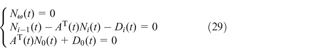
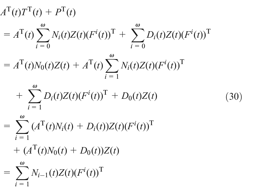
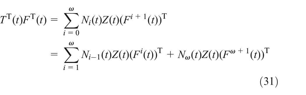
Let us introduce the solution to the first-order homogeneous GSE with time-varying coefficients

V (t) F = A (t) V (t) + B (t) W (t)

(1)

where $A (t) \in R^{n \times q}$ , $B (t) \in R^{n \times r}$ , $q + r > n$ and $F \in C^{p \times p}$ are coefficient matrices, and $V (t) \in C^{q \times p}$ , $W (t) \in C^{r \times p}$ are parameter matrices of required solutions.

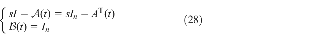
Definition 1. (Duan, 2014) The pair ${sI - A (t), B (t)}$ are called left coprime with rank $α$ over $J$ if the pair ${sI - A (t), B (t)}$ are $F$ -left coprime with rank $α$ for arbitrary $F \in C^{p \times p}$ , that is,

rank [\begin{matrix} sI - A (t) & B (t) \end{matrix}] = α, \forall t \in J, s \in eig (F)

(2)

According to Definition 1, when the rank condition (2) is met, there are unimodular matrices $P (t, s)$ and $Q (t, s)$ satisfying the following equation

P (t, s) [\begin{matrix} sI - A (t) & - B (t) \end{matrix}] Q (t, s) = [\begin{matrix} Σ (t, s) & 0 \end{matrix}]

(3)

where $Σ (t, s) \in R^{α \times α} [s]$ is usually diagonal and satisfies

\det Σ (t, s) \neq 0, \forall t \in J, s \in eig (F)

and $Q (t, s)$ can be partitioned as

Q (t, s) = [\begin{matrix} * & N (t, s) \\ * & D (t, s) \end{matrix}]

with $D (t, s) \in R^{r \times β_{0}} [s]$ and $N (t, s) \in R^{q \times β_{0}} [s]$ , $β_{0} = q + r - n$ , then equation (3) leads to

(sI - A (t)) N (t, s) - B (t) D (t, s) = 0

(4)

Moreover, when $q = n$ , that is $A (t)$ is invertible, we have $α = n$ , and the above equation can be rewritten in the form of

{(sI - A (t))}^{- 1} B (t) - N (t, s) D^{- 1} (t, s) = 0

(5)

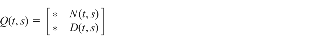
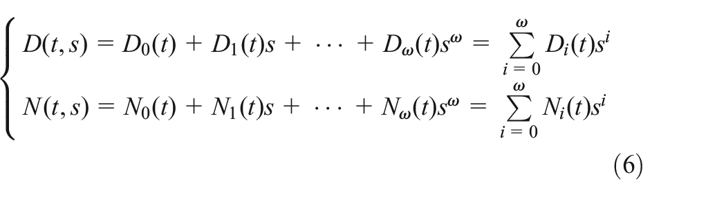
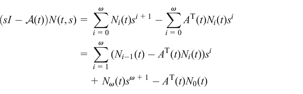
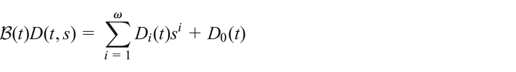
This is well-known right coprime factorization (RCF) of the matrix pair ${sI - A (t), B (t)}$ (Duan, 2014). Considering the physical realizability of $N (t, s) D^{- 1} (t, s)$ , the maximum degree of polynomial matrices $D (t, s)$ and $N (t, s)$ is determined by that of $D (t, s)$ . Furthermore, let $ω$ be the maximum degree of $D (t, s)$ , then $D (t, s)$ and $N (t, s)$ can be rewritten as

{\begin{matrix} D (t, s) = D_{0} (t) + D_{1} (t) s + \dots + D_{ω} (t) s^{ω} = \sum_{i = 0}^{ω} D_{i} (t) s^{i} \\ N (t, s) = N_{0} (t) + N_{1} (t) s + \dots + N_{ω} (t) s^{ω} = \sum_{i = 0}^{ω} N_{i} (t) s^{i} \end{matrix}

(6)

For the solution to GSE (1), we have the following results hold.

Theorem 1 (Duan, 2014) Let $F \in C^{p \times p}$ , and the pair ${sI - A (t), B (t)}$ be $F$ -left coprime over $J$ . Furthermore, given $D (t, s)$ and $N (t, s)$ are right coprime polynomial matrices satisfy equation (5)and have the form of equation (6). Then, for $t \in J$ , a general solution to the GSE (1) is

{\begin{matrix} W (t) = D_{0} (t) Z + D_{1} (t) Z F + \dots + D_{ω} (t) Z F^{ω} = \sum_{i = 0}^{ω} D_{i} (t) Z F^{i} \\ V (t) = N_{0} (t) Z + N_{1} (t) Z F + \dots + N_{ω} (t) Z F^{ω} = \sum_{i = 0}^{ω} N_{i} (t) Z F^{i} \end{matrix}

(7)

where $Z \in C^{β_{0} \times p}$ is an arbitrary parameter matrix.

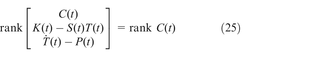
Problem statement

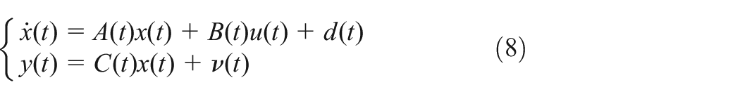
The LTV system with additional disturbances can be described as

{\begin{matrix} \overset{\cdot}{x} (t) = A (t) x (t) + B (t) u (t) + d (t) \\ y (t) = C (t) x (t) + ν (t) \end{matrix}

(8)

where $x (t) \in R^{n}$ , $u (t) \in R^{r}$ , $d (t) \in R^{n}$ , and $y (t) \in R^{m}$ represent state, input, bounded disturbance, and output, respectively. $ν \in ι_{\infty}^{m}$ is the output disturbance, $A (t)$ , $B (t)$ , and $C (t)$ are known and continuous for time $t$ .

Assumption 1. $x (t) \in ι_{\infty}^{m}$ with ${\underline{x}}_{0} \leq x_{0} \leq {\bar{x}}_{0}$ for some ${\underline{x}}_{0}, {\bar{x}}_{0} \in C$ .

Assumption 2. $\underline{d} (t) \leq d (t) \leq \bar{d} (t)$ with known $\underline{d} (t), \bar{d} (t) \in ι_{\infty}^{m}$ .

Assumption 3. $| | ν (t) | | \leq \bar{ν}$ for a given $\bar{ν} > 0$ .

We concentrate on the estimation for functional signal

h (t) = K (t) x (t)

(9)

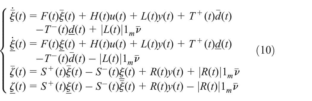
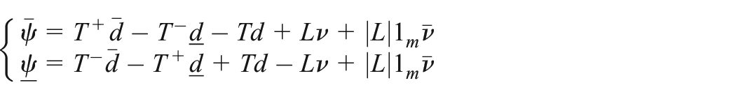
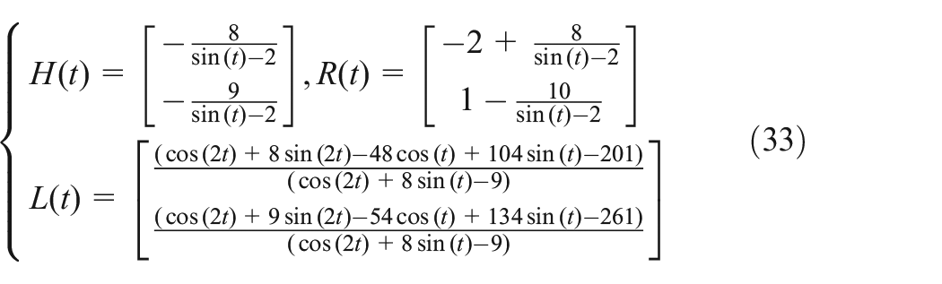
with a known $K (t) \in R^{k \times n}$ , then above target can be realized by using the following Luenberger-like FIO system

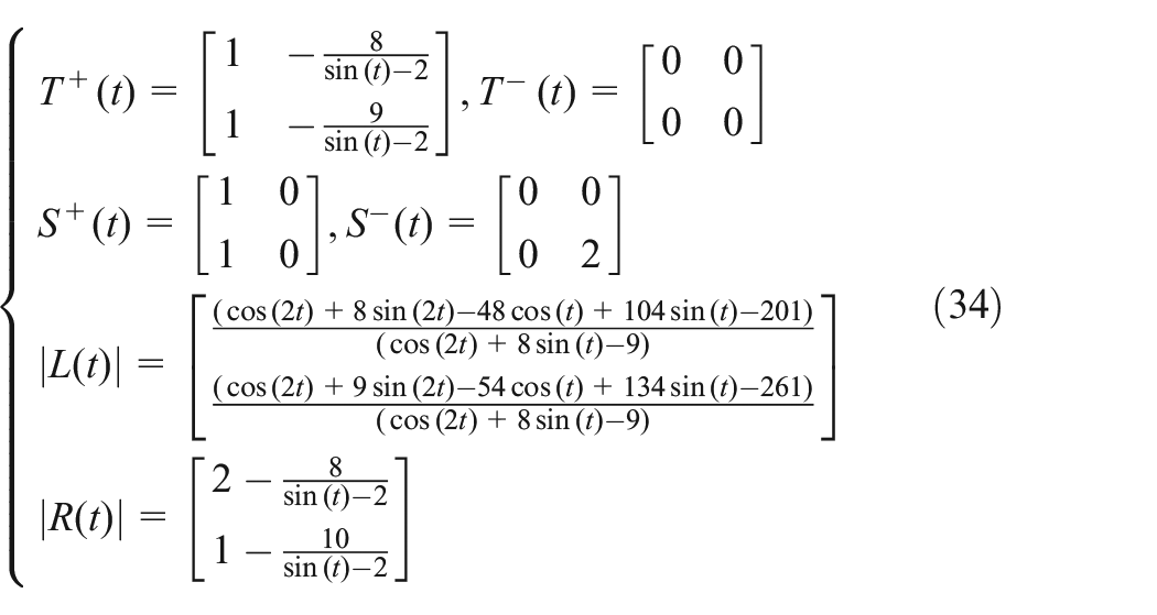
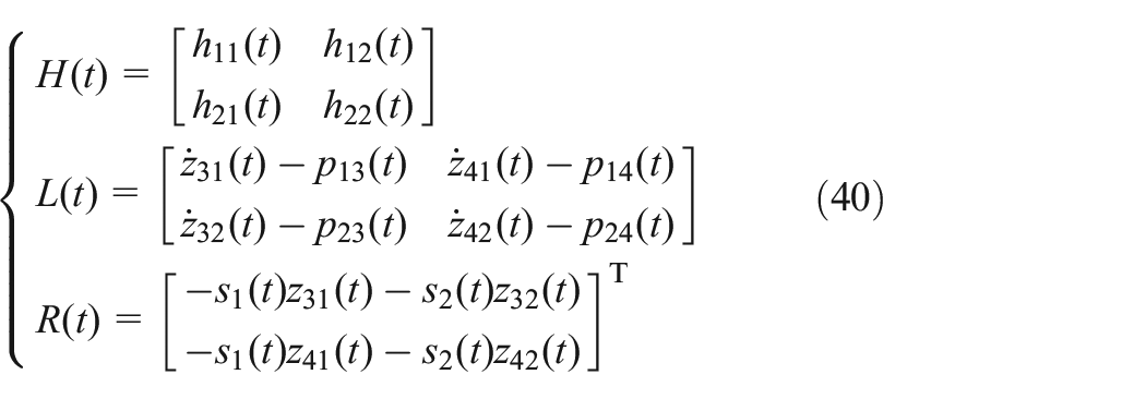
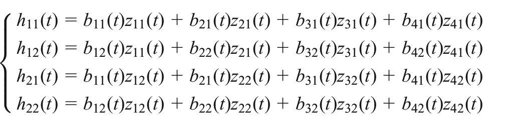
{\begin{matrix} \overset{\cdot}{\bar{ξ}} (t) = F (t) \bar{ξ} (t) + H (t) u (t) + L (t) y (t) + T^{+} (t) \bar{d} (t) \\ - T^{-} (t) \underline{d} (t) + | L (t {) | 1}_{m} \bar{ν} \\ \underline{\overset{\cdot}{ξ}} (t) = F (t) \underline{ξ} (t) + H (t) u (t) + L (t) y (t) + T^{+} (t) \underline{d} (t) \\ - T^{-} (t) \bar{d} (t) - | L (t {) | 1}_{m} \bar{ν} \\ \bar{ζ} (t) = S^{+} (t) \bar{ξ} (t) - S^{-} (t) \underline{ξ} (t) + R (t) y (t) + | R (t {) | 1}_{m} \bar{ν} \\ \underline{ζ} (t) = S^{+} (t) \underline{ξ} (t) - S^{-} (t) \bar{ξ} (t) + R (t) y (t) - | R (t {) | 1}_{m} \bar{ν} \end{matrix}

(10)

where $\bar{ξ} (t)$ and $\underline{ξ} (t)$ are $μ$ -dimensional observer state vectors as well as $\bar{ζ} (t)$ and $\underline{ζ} (t)$ are $k$ -dimensional observer output vectors. Matrices $F (t)$ , $H (t)$ , $L (t)$ , and $R (t)$ are unknowns to be determined. The construction of $S^{+} (t)$ , $S^{-} (t)$ , $T^{+} (t)$ , and $T^{-} (t)$ depends on the values of matrices $S (t)$ and $T (t)$ , which also need to be solved.

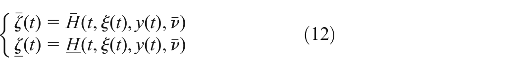
Definition 2. Under the premise that Assumptions 1–3 are all true, system

\overset{\cdot}{ξ} (t) = F (ξ (t), u (t), y (t), \bar{ν}, \bar{d} (t), \underline{d} (t))

(11)

with outputs

{\begin{matrix} \bar{ζ} (t) = \bar{H} (t, ξ (t), y (t), \bar{ν}) \\ \underline{ζ} (t) = \underline{H} (t, ξ (t), y (t), \bar{ν}) \end{matrix}

(12)

is called an FIO of $h (t)$ for system (8) if

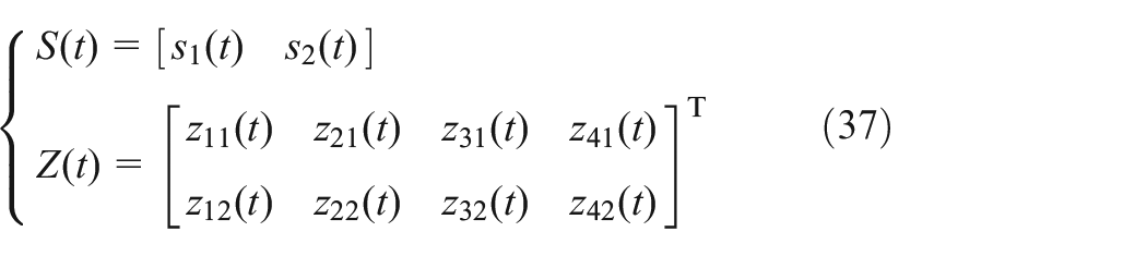
1. Dynamical system (8) satisfies the stable input state;

2. The functional $h (t)$ and output $\bar{ζ} (t)$ , $\underline{ζ} (t)$ of system (9) and (12) satisfy the following inequality relationship

\underline{ζ} (t) \leq h (t) \leq \bar{ζ} (t), t \in J

3. If $| | \bar{d} (t) - \underline{d} (t) | |$ and $| | ν (t) | |$ are uniformly bounded, then $| | \bar{ζ} (t) - \underline{ζ} (t) | |$ uniformly bounded. If $| | \bar{d} (t) - \underline{d} (t) | |$ and $| | ν (t) | |$ both converge to zero over $J$ , then $| | \bar{ζ} (t) - \underline{ζ} (t) | |$ also converges to zero.

The main work of this paper is to propose sufficient conditions for the existence of Luenberger-like FIO system (10) and obtain the corresponding gain matrices and then construct the observer system to complete the interval estimation of $h (t)$ for system (8).

Main results

Existence conditions for FIO system

In this section, we will discuss the sufficient conditions to make the observation error dynamic system non-negative, ensuring that the observer (10) becomes an FIO of system (8). In this regard, following existence theorem holds.

Theorem 2. Assuming that system (8) is observable and satisfies Assumptions 1–3, then dynamic system (10) is a functional interval estimator of equation (8) if

F (t) is Metzler and Hurwitz

(13)

\overset{\cdot}{T} (t) + T (t) A (t) - L (t) C (t) = F (t) T (t)

(14)

K (t) - S (t) T (t) = R (t) C (t)

(15)

H (t) = T (t) B (t)

(16)

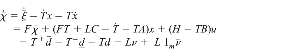
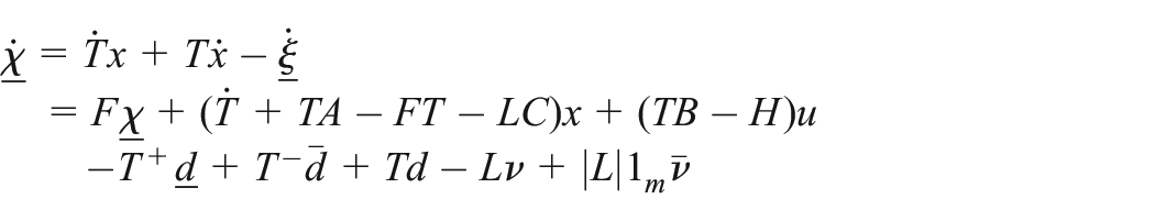
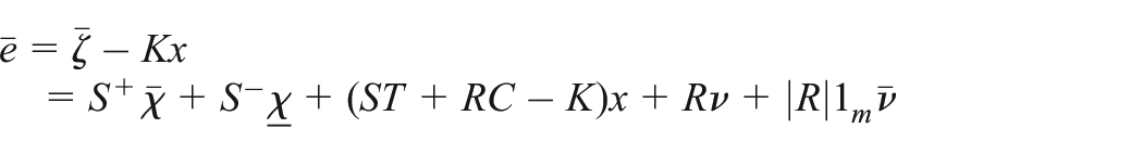
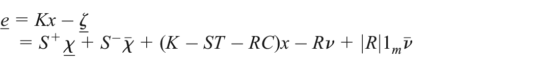
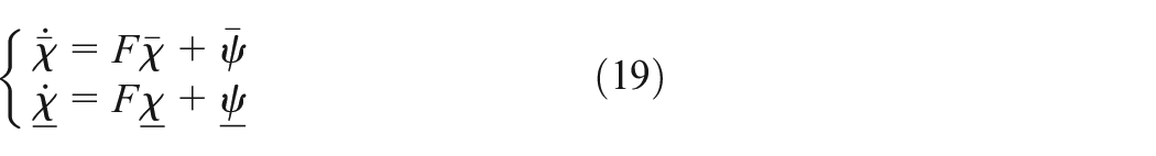
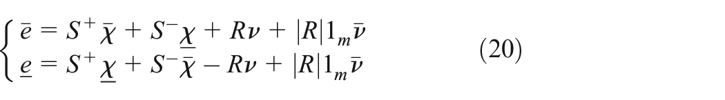
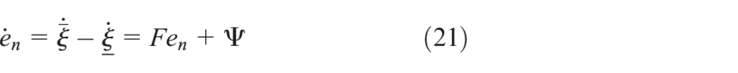
Proof. For the sake of brevity, the explicit time dependency has been removed from our notations. Denote

\bar{χ} = \bar{ξ} - Tx, \underline{χ} = Tx - \underline{ξ}

(17)

and

\bar{e} = \bar{ζ} - Kx, \underline{e} = Kx - \underline{ζ}

(18)

Taking the derivative of equation (17), we get

\begin{matrix} \overset{\cdot}{\bar{χ}} = \overset{\cdot}{\bar{ξ}} - \overset{\cdot}{T} x - T \overset{\cdot}{x} \\ = F \bar{χ} + (FT + LC - \overset{\cdot}{T} - TA) x + (H - TB) u \\ + T^{+} \bar{d} - T^{-} \underline{d} - Td + L ν + | L {| 1}_{m} \bar{ν} \end{matrix}

and

\begin{matrix} \underline{\overset{\cdot}{χ}} = \overset{\cdot}{T} x + T \overset{\cdot}{x} - \underline{\overset{\cdot}{ξ}} \\ = F \underline{χ} + (\overset{\cdot}{T} + TA - FT - LC) x + (TB - H) u \\ - T^{+} \underline{d} + T^{-} \bar{d} + Td - L ν + | L {| 1}_{m} \bar{ν} \end{matrix}

Furthermore, by transforming and substituting it into equation (18) yields

\begin{matrix} \bar{e} = \bar{ζ} - Kx \\ = S^{+} \bar{χ} + S^{-} \underline{χ} + (ST + RC - K) x + R ν + | R {| 1}_{m} \bar{ν} \end{matrix}

and

\begin{matrix} \underline{e} = Kx - \underline{ζ} \\ = S^{+} \underline{χ} + S^{-} \bar{χ} + (K - ST - RC) x - R ν + | R {| 1}_{m} \bar{ν} \end{matrix}

Then, $F (t)$ is Metzler and Hurwitz and equations (14)–(16) hold, we can obtain

{\begin{matrix} \overset{\cdot}{\bar{χ}} = F \bar{χ} + \bar{ψ} \\ \underline{\overset{\cdot}{χ}} = F \underline{χ} + \underline{ψ} \end{matrix}

(19)

and

{\begin{matrix} \bar{e} = S^{+} \bar{χ} + S^{-} \underline{χ} + R ν + | R {| 1}_{m} \bar{ν} \\ \underline{e} = S^{+} \underline{χ} + S^{-} \bar{χ} - R ν + | R {| 1}_{m} \bar{ν} \end{matrix}

(20)

with

{\begin{matrix} \bar{ψ} = T^{+} \bar{d} - T^{-} \underline{d} - Td + L ν + | L {| 1}_{m} \bar{ν} \\ \underline{ψ} = T^{-} \bar{d} - T^{+} \underline{d} + Td - L ν + | L {| 1}_{m} \bar{ν} \end{matrix}

According to Lemma 1 and Assumption 3, there are $\bar{χ} \geq 0$ and $\underline{χ} \geq 0$ . Furthermore, from (20) $\bar{e} \geq 0$ and $\underline{e} \geq 0$ hold, that is

\underline{ζ} \leq h = Kx \leq \bar{ζ}

Next, denote $e_{n} = \bar{ξ} - \underline{ξ}$ and $e = \bar{ζ} - \underline{ζ}$ represent observer state interval and output interval, respectively. Then

{\overset{\cdot}{e}}_{n} = \overset{\cdot}{\bar{ξ}} - \underline{\overset{\cdot}{ξ}} = F e_{n} + Ψ

(21)

e = \bar{ζ} - \underline{ζ} = | S | e_{n} + 2 | R | 1_{m} \bar{ν}

(22)

with $Ψ = | T | (\bar{d} - \underline{d}) + 2 | L | 1_{m} \bar{ν}$ . Since the matrix $F$ is Metzler and Hurwitz, that means $λ (F) < 0$ , when $| | \bar{d} - \underline{d} | |$ and $| L | 1_{m} \bar{ν}$ are uniformly bounded over $J$ , then $e_{n}$ converges asymptotically to $e_{\max}$ , that also means $e$ is asymptotically converges and bounded; when $| | \bar{d} - \underline{d} | |$ and $| L | 1_{m} \bar{ν}$ both converge to zero over $J$ , then $e$ converges to zero, namely, the output interval of the observer system is asymptotically stable. Thus, the proof is completed.

Remark 1. From the proof of Theorem 2, we get that the design of observer error matrix is independent, and the Metzler and Hurwitz matrix $F (t)$ can be assigned any value. That is, the stability of observer is guaranteed by an arbitrarily structured Metzler and Hurwitz matrix $F (t)$ , which reduces the conservativeness of this design method. Furthermore, according to equations (21) and (22), the error will converge to a non-negative bounded interval over time, where the convergence rate is controlled by $F (t)$ and $Ψ (t)$ , and the interval width is determined by $R (t)$ and $ν (t)$ .

Parametric forms of observer gain matrices

The parametric design provides all the degrees of freedom; therefore, we propose a parametric design method for the FIO of the LTV system (8) with additional disturbances in the form of equation (10). Based on the existence conditions presented in the previous section, parameterized expressions of observer gain are shown below.

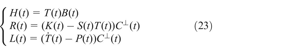
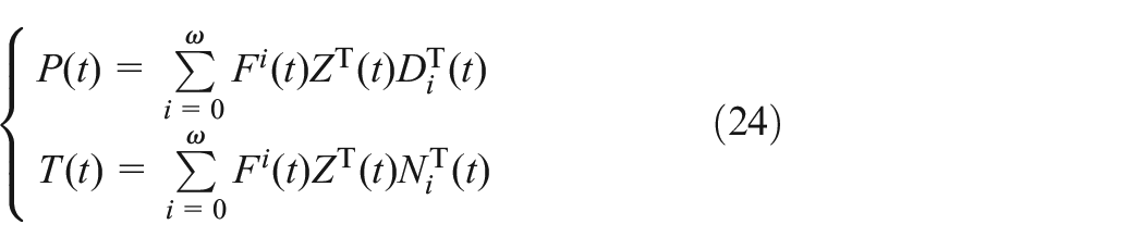
Theorem 3. Given the observable system (8) satisfying Assumptions 1–3 and $F (t) \in R^{μ \times μ}$ is an arbitrary Metzler and Hurwitz matrix, $D (t, s)$ and $N (t, s)$ are right coprime polynomial matrices in the forms of equation (6) and satisfying equation (5) with $A (t) = A^{T} (t)$ , $B (t) = I_{n}$ . Then, the fully parameterized expressions of the coefficient matrices of FIO (10) are

{\begin{matrix} H (t) = T (t) B (t) \\ R (t) = (K (t) - S (t) T (t)) C^{⊥} (t) \\ L (t) = (\overset{\cdot}{T} (t) - P (t)) C^{⊥} (t) \end{matrix}

(23)

where

{\begin{matrix} P (t) = \sum_{i = 0}^{ω} F^{i} (t) Z^{T} (t) D_{i}^{T} (t) \\ T (t) = \sum_{i = 0}^{ω} F^{i} (t) Z^{T} (t) N_{i}^{T} (t) \end{matrix}

(24)

and there are two arbitrary matrices $Z (t) \in R^{n \times μ}$ , $S (t) \in R^{k \times μ}$ such that

rank [\begin{matrix} C (t) \\ K (t) - S (t) T (t) \\ \overset{\cdot}{T} (t) - P (t) \end{matrix}] = rank C (t)

(25)

Proof. Proof of this theorem consists of two steps.

Step 1. Parameterized expression of matrices $P (t)$ and $T (t)$ .

Denote

P (t) = \overset{\cdot}{T} (t) - L (t) C (t)

(26)

substituting equation (26) into equation (14), by transposing we obtain the following GSE

A^{T} (t) T^{T} (t) + P^{T} (t) = T^{T} (t) F^{T} (t)

(27)

and corresponding polynomials in equation (4) are

{\begin{matrix} sI - A (t) = s I_{n} - A^{T} (t) \\ B (t) = I_{n} \end{matrix}

(28)

Using equation(6), we have

\begin{matrix} (sI - A (t)) N (t, s) = \sum_{i = 0}^{ω} N_{i} (t) s^{i + 1} - \sum_{i = 0}^{ω} A^{T} (t) N_{i} (t) s^{i} \\ = \sum_{i = 1}^{ω} (N_{i - 1} (t) - A^{T} (t) N_{i} (t)) s^{i} \\ + N_{ω} (t) s^{ω + 1} - A^{T} (t) N_{0} (t) \end{matrix}

and

B (t) D (t, s) = \sum_{i = 1}^{ω} D_{i} (t) s^{i} + D_{0} (t)

Substituting the above two relations into equation (4), then

{\begin{matrix} N_{ω} (t) = 0 \\ N_{i - 1} (t) - A^{T} (t) N_{i} (t) - D_{i} (t) = 0 \\ A^{T} (t) N_{0} (t) + D_{0} (t) = 0 \end{matrix}

(29)

Using equations (24) and (27), we can obtain

\begin{matrix} A^{T} (t) T^{T} (t) + P^{T} (t) \\ = A^{T} (t) \sum_{i = 0}^{ω} N_{i} (t) Z (t) (F^{i} (t {))}^{T} + \sum_{i = 0}^{ω} D_{i} (t) Z (t) (F^{i} (t {))}^{T} \\ = A^{T} (t) N_{0} (t) Z (t) + A^{T} (t) \sum_{i = 1}^{ω} N_{i} (t) Z (t) (F^{i} (t {))}^{T} \\ + \sum_{i = 1}^{ω} D_{i} (t) Z (t) (F^{i} (t {))}^{T} + D_{0} (t) Z (t) \\ = \sum_{i = 1}^{ω} (A^{T} (t) N_{i} (t) + D_{i} (t)) Z (t) (F^{i} (t {))}^{T} \\ + (A^{T} (t) N_{0} (t) + D_{0} (t)) Z (t) \\ = \sum_{i = 1}^{ω} N_{i - 1} (t) Z (t) (F^{i} (t {))}^{T} \end{matrix}

(30)

and

\begin{matrix} T^{T} (t) F^{T} (t) = \sum_{i = 0}^{ω} N_{i} (t) Z (t) (F^{i + 1} (t {))}^{T} \\ = \sum_{i = 1}^{ω} N_{i - 1} (t) Z (t) (F^{i} (t {))}^{T} + N_{ω} (t) Z (t) (F^{ω + 1} (t {))}^{T} \end{matrix}

(31)

Using the relations in equation (29), it is easy to see that the right-hand sides of the above two equations are equal. This states that the expressions in equation (24) satisfy equation (27), and we can have the parametric solutions of $P (t)$ and $T (t)$ as shown in equation (24) with a given Metzler and Hurwitz matrix $F (t)$ .

Step 2. Parameterized expression of matrices $H (t)$ , $R (t)$ , and $L (t)$ .

Obviously, the matrices $H (t)$ , $R (t)$ , and $L (t)$ are determined by equations (15), (16), and (26), combining these equations produces (23). In particular, there are $R (t)$ and $L (t)$ if and only if the expression (25) is established. At this point, proof of the theorem is completed.

Remark 2. For observer system (10), Theorem 3 gives all the gains that satisfy the most basic requirements, where there is a set of free parameter $Z (t)$ . Because of its existence, the above condition (25) is easily met, and other design requirements can also be reached by choosing $Z (t)$ .

Design algorithm

In this section, we propose the following algorithm for parameterized design of an FIO of LTV system (8) in the form of equation (10).

Step 1: Choose $F (t)$ as an arbitrary Metzler and Hurwitz matrix. Generally, it is selected as a diagonal form to facilitate the judgment of stability.

Step 2: Solve right coprime matrices $D (t, s)$ and $N (t, s)$ satisfying RCF (5), the form of which are shown in equation (6).

Step 3: Obtain the matrices $P (t)$ and $T (t)$ from equation (24), check if there exists parameter matrix $Z (t)$ to make (25) true. If not, return to Step 1 and select $F (t)$ again, if yes, proceed to the next step.

Step 4: Complete the coefficient matrices $H (t)$ , $R (t)$ and $L (t)$ through Theorem 3, then obtain matrices $S^{+} (t)$ , $S^{-} (t)$ , $T^{+} (t)$ , and $T^{-} (t)$ to finish the structure of observer (10).

Remark 3. The main computations of the above algorithm contain the calculation of RCF (4) and the solution of a set of linear matrix equations. Also note that solving the GSE (27) involves the value of matrix $F (t)$ , and the constraint on $F (t)$ is just an arbitrary Metzler and Hurwitz matrix, it may be chosen as a constant form in the application for the purpose of simplifying the calculation. Furthermore, the design parameter $Z (t)$ can be reasonably selected to make the control system have other desired performances under the condition that the basic requirements are met.

Examples

Numerical simulation

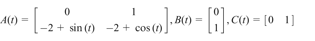
This section presents a numerical example to demonstrate the effectiveness and correctness of the designed algorithm. Consider the following first-order observable LTV system with the coefficient matrices

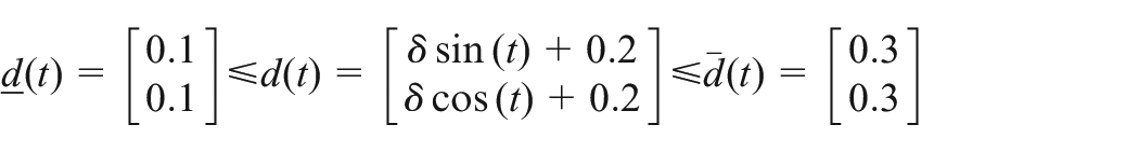
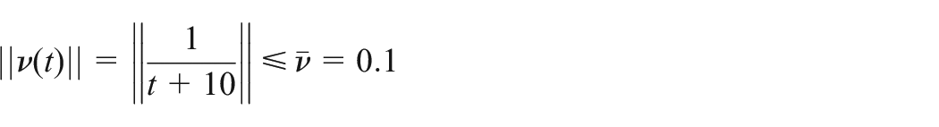
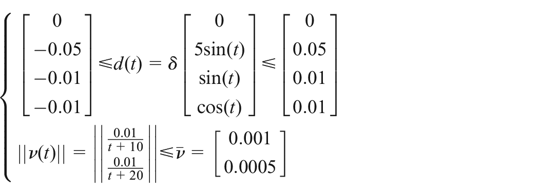
\begin{matrix} A (t) = [\begin{matrix} 0 & 1 \\ - 2 + \sin (t) & - 2 + \cos (t) \end{matrix}], B (t) = [\begin{matrix} 0 \\ 1 \end{matrix}], C (t) = [\begin{matrix} 0 & 1 \end{matrix}] \end{matrix}

Assuming the presence of bounded perturbations

\underline{d} (t) = [\begin{matrix} 0.1 \\ 0.1 \end{matrix}] \leq d (t) = [\begin{matrix} δ \sin (t) + 0.2 \\ δ \cos (t) + 0.2 \end{matrix}] \leq \bar{d} (t) = [\begin{matrix} 0.3 \\ 0.3 \end{matrix}]

and output perturbations

| | ν (t) | | = ‖ \frac{1}{t + 10} ‖ \leq \bar{ν} = 0.1

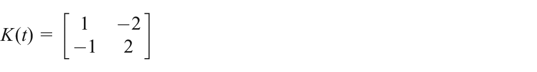
where $δ = 0.01$ . We design to estimate the following signal $K (t) x (t)$ , where

K (t) = [\begin{matrix} 1 & - 2 \\ - 1 & 2 \end{matrix}]

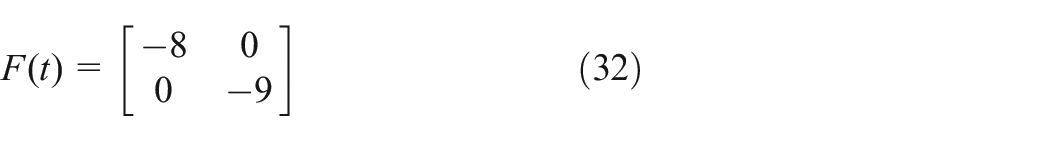
Select the Metzler and Hurwitz matrix $F (t)$ as the following constant form

F (t) = [\begin{matrix} - 8 & 0 \\ 0 & - 9 \end{matrix}]

(32)

then following matrices are obtained according to Theorem 3

\begin{matrix} {\begin{matrix} H (t) = [\begin{matrix} - \frac{8}{\sin (t) - 2} \\ - \frac{9}{\sin (t) - 2} \end{matrix}], R (t) = [\begin{matrix} - 2 + \frac{8}{\sin (t) - 2} \\ 1 - \frac{10}{\sin (t) - 2} \end{matrix}] \\ L (t) = [\begin{matrix} \frac{(\cos (2 t) + 8 \sin (2 t) - 48 \cos (t) + 104 \sin (t) - 201)}{(\cos (2 t) + 8 \sin (t) - 9)} \\ \frac{(\cos (2 t) + 9 \sin (2 t) - 54 \cos (t) + 134 \sin (t) - 261)}{(\cos (2 t) + 8 \sin (t) - 9)} \end{matrix}] \end{matrix} \end{matrix}

(33)

and the other coefficient matrices of the observer (10) are

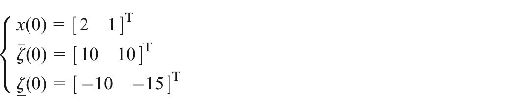
\begin{matrix} {\begin{matrix} T^{+} (t) = [\begin{matrix} 1 & - \frac{8}{\sin (t) - 2} \\ 1 & - \frac{9}{\sin (t) - 2} \end{matrix}], T^{-} (t) = [\begin{matrix} 0 & 0 \\ 0 & 0 \end{matrix}] \\ S^{+} (t) = [\begin{matrix} 1 & 0 \\ 1 & 0 \end{matrix}], S^{-} (t) = [\begin{matrix} 0 & 0 \\ 0 & 2 \end{matrix}] \\ | L (t) | = [\begin{matrix} \frac{(\cos (2 t) + 8 \sin (2 t) - 48 \cos (t) + 104 \sin (t) - 201)}{(\cos (2 t) + 8 \sin (t) - 9)} \\ \frac{(\cos (2 t) + 9 \sin (2 t) - 54 \cos (t) + 134 \sin (t) - 261)}{(\cos (2 t) + 8 \sin (t) - 9)} \end{matrix}] \\ | R (t) | = [\begin{matrix} 2 - \frac{8}{\sin (t) - 2} \\ 1 - \frac{10}{\sin (t) - 2} \end{matrix}] \end{matrix} \end{matrix}

(34)

Choose the initial condition as

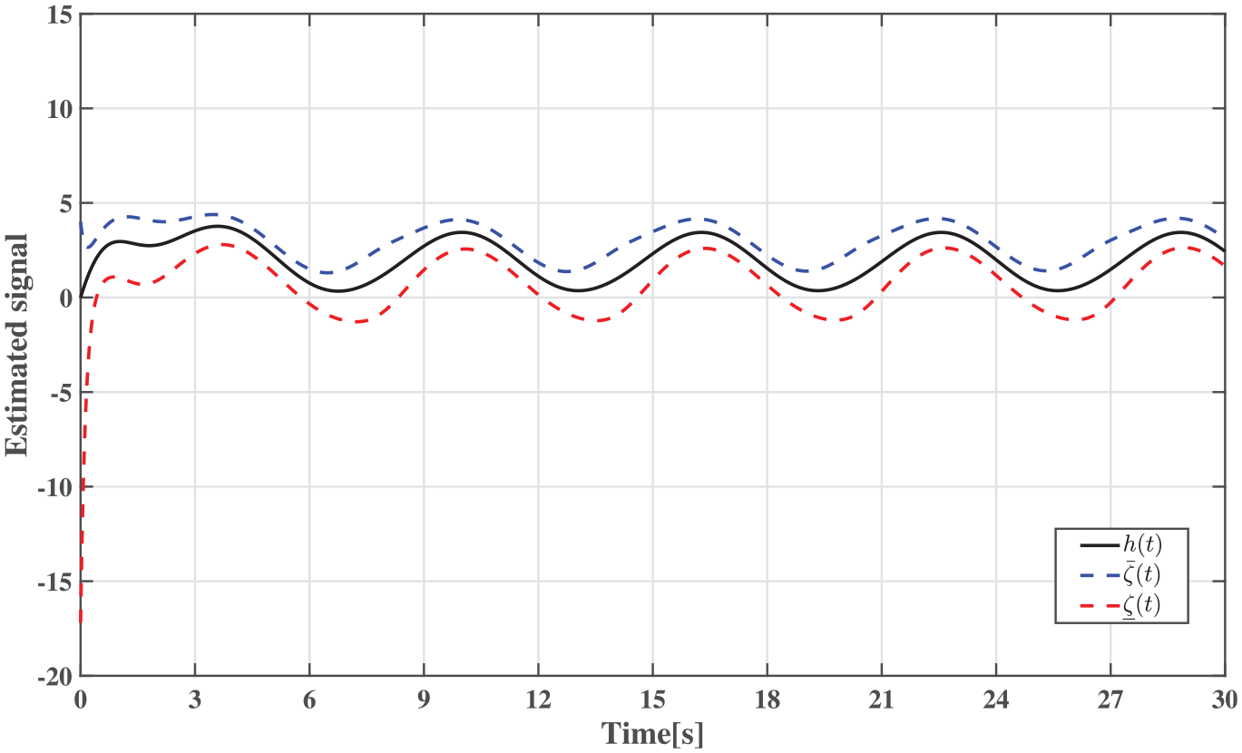
\begin{matrix} {\begin{matrix} x (0) = {[\begin{matrix} 2 & 1 \end{matrix}]}^{T} \\ \bar{ζ} (0) = {[\begin{matrix} 10 & 10 \end{matrix}]}^{T} \\ \underline{ζ} (0) = {[\begin{matrix} - 10 & - 15 \end{matrix}]}^{T} \end{matrix} \end{matrix}

without loss of generality, choose the control input as $u (t) = 2$ , $0 \leq t \leq 30$ . The simulation results are plotted in Figures 1 and 2.

Figure 1.

Observation effect of the designed observer on signal 1.

Figure 2.

Observation effect of the designed observer on signal 2.

Figures 1 and 2 show the observation effect of the interval observer proposed in this paper on two function signals. It can be seen from these two figures that the FIO designed based on the parameterization method accomplishes the task of interval estimation very well, which shows the effectiveness of proposed method.

Aircraft control system

This section takes the FIO design for BTT aircraft control system as an example to verify the proposed method. Duan and Wang (2005) presented the mathematical model of BTT missile pitch/yaw channel autopilot as

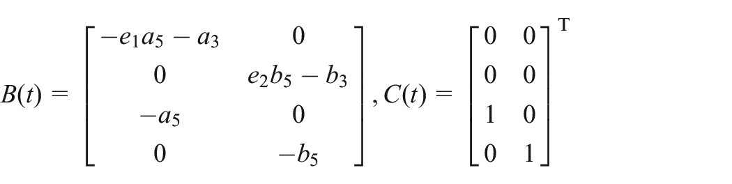
\begin{matrix} A (t) = [\begin{matrix} - a_{1} - e_{1} & \frac{(J_{x} - J_{y}) ω_{x}}{57.3 J_{z}} & e_{1} a_{4} - a_{2} & \frac{e_{1} ω_{x}}{57.3} \\ \frac{(J_{z} - J_{x}) ω_{x}}{57.3 J_{y}} & - b_{1} - e_{2} & \frac{- e_{2} ω_{x}}{57.3} & e_{2} b_{4} - b_{2} \\ 1 & 0 & - a_{4} & \frac{- ω_{x}}{57.3} \\ 0 & 1 & \frac{ω_{x}}{57.3} & - b_{4} \end{matrix}] \end{matrix}

\begin{matrix} B (t) = [\begin{matrix} - e_{1} a_{5} - a_{3} & 0 \\ 0 & e_{2} b_{5} - b_{3} \\ - a_{5} & 0 \\ 0 & - b_{5} \end{matrix}], C (t) = {[\begin{matrix} 0 & 0 \\ 0 & 0 \\ 1 & 0 \\ 0 & 1 \end{matrix}]}^{T} \end{matrix}

where state $x = [ω_{z}, ω_{y}, α, β]^{T}$ , input $u = [δ_{z}, δ_{y}]^{T}$ , and output $y = [α, β]^{T}$ . $ω_{x}$ , $ω_{y}$ , $ω_{z}$ are the components of angular velocity on the three axes of the projectile coordinate system; $α$ , $β$ are the angle of attack and sideslip; $δ_{z}$ , $δ_{y}$ represent the yaw angle of the pitch rudder surface and the yaw rudder surface; $J_{x}$ , $J_{y}$ , $J_{z}$ are the moments of inertia of the missile relative to the three axes of projectile coordinate system. Parameters $a_{i} (t)$ , $b_{i} (t)$ , and $e_{i} (t)$ are functions of the time $t$ that change with altitude and speed. Assume there exist disturbances $d (t)$ and $ν (t)$ satisfying Assumptions 2 and 3, and the linear function is given by

K (t) = [\begin{matrix} k_{1} (t) & k_{2} (t) & 0 & 0 \end{matrix}]

with $k_{1} (t) k_{2} (t) \neq 0$ over $J$ .

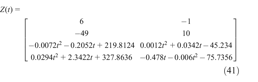
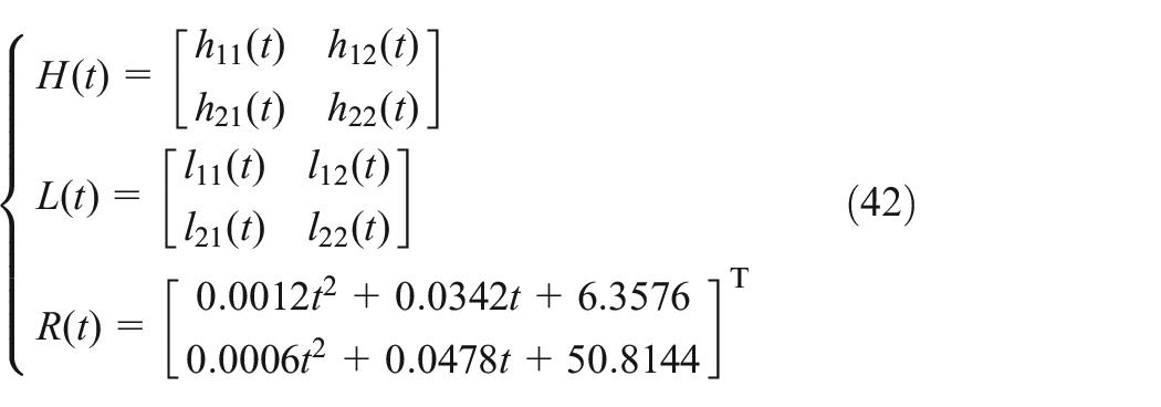
In the following part, for the convenience of narration, we denote matrices $A (t) = [a_{ij} (t)]$ and $B (t) = [b_{ij} (t)]$ . For these, matrices $D (t, s)$ and $N (t, s)$ satisfying (5) can be chosen as

\begin{matrix} {\begin{matrix} D (t, s) = [\begin{matrix} s - a_{11} (t) & - a_{21} (t) & - a_{31} (t) & - a_{41} (t) \\ - a_{12} (t) & s - a_{22} (t) & - a_{32} (t) & - a_{42} (t) \\ - a_{13} (t) & - a_{23} (t) & s - a_{33} (t) & - a_{43} (t) \\ - a_{14} (t) & - a_{24} (t) & - a_{34} (t) & s - a_{44} (t) \end{matrix}] \\ N (t, s) = I_{4} \end{matrix} \end{matrix}

(35)

According to Theorem 3, to simplify the calculation, we select the Metzler and Hurwitz matrix $F (t)$ as the following constant form

F (t) = [\begin{matrix} - 8 & 0 \\ 0 & - 9 \end{matrix}]

(36)

and denote

\begin{matrix} {\begin{matrix} S (t) = [\begin{matrix} s_{1} (t) & s_{2} (t) \end{matrix}] \\ Z (t) = {[\begin{matrix} z_{11} (t) & z_{21} (t) & z_{31} (t) & z_{41} (t) \\ z_{12} (t) & z_{22} (t) & z_{32} (t) & z_{42} (t) \end{matrix}]}^{T} \end{matrix} \end{matrix}

(37)

Then, substituting equations (35)–(37) into equation (24), we get

\begin{matrix} {\begin{matrix} P (t) = [\begin{matrix} p_{11} (t) & p_{12} (t) & p_{13} (t) & p_{14} (t) \\ p_{21} (t) & p_{22} (t) & p_{23} (t) & p_{24} (t) \end{matrix}] \\ T (t) = [\begin{matrix} z_{11} (t) & z_{21} (t) & z_{31} (t) & z_{41} (t) \\ z_{12} (t) & z_{22} (t) & z_{32} (t) & z_{42} (t) \end{matrix}] \end{matrix} \end{matrix}

(38)

with

\begin{matrix} {\begin{matrix} p_{11} (t) = - 8 z_{11} (t) - a_{11} (t) z_{11} (t) - a_{21} (t) z_{21} (t) - a_{31} (t) z_{31} (t) - a_{41} (t) z_{41} (t) \\ p_{12} (t) = - 8 z_{21} (t) - a_{12} (t) z_{11} (t) - a_{22} (t) z_{21} (t) - a_{32} (t) z_{31} (t) - a_{42} (t) z_{41} (t) \\ p_{13} (t) = - 8 z_{31} (t) - a_{13} (t) z_{11} (t) - a_{23} (t) z_{21} (t) - a_{33} (t) z_{31} (t) - a_{43} (t) z_{41} (t) \\ p_{14} (t) = - 8 z_{41} (t) - a_{14} (t) z_{11} (t) - a_{24} (t) z_{21} (t) - a_{34} (t) z_{31} (t) - a_{44} (t) z_{41} (t) \\ p_{21} (t) = - 9 z_{12} (t) - a_{11} (t) z_{12} (t) - a_{21} (t) z_{22} (t) - a_{31} (t) z_{32} (t) - a_{41} (t) z_{42} (t) \\ p_{22} (t) = - 9 z_{22} (t) - a_{12} (t) z_{12} (t) - a_{22} (t) z_{22} (t) - a_{32} (t) z_{32} (t) - a_{42} (t) z_{42} (t) \\ p_{23} (t) = - 9 z_{32} (t) - a_{13} (t) z_{12} (t) - a_{23} (t) z_{22} (t) - a_{33} (t) z_{32} (t) - a_{43} (t) z_{42} (t) \\ p_{24} (t) = - 9 z_{42} (t) - a_{14} (t) z_{12} (t) - a_{24} (t) z_{22} (t) - a_{34} (t) z_{32} (t) - a_{44} (t) z_{42} (t) \end{matrix} \end{matrix}

and equation (25) leads

\begin{matrix} {\begin{matrix} k_{1} (t) - s_{1} (t) z_{11} (t) - s_{2} (t) z_{12} (t) = 0 \\ k_{2} (t) - s_{1} (t) z_{21} (t) - s_{2} (t) z_{22} (t) = 0 \\ {\overset{\cdot}{z}}_{11} (t) - p_{11} (t) = 0 \\ {\overset{\cdot}{z}}_{21} (t) - p_{12} (t) = 0 \\ {\overset{\cdot}{z}}_{12} (t) - p_{21} (t) = 0 \\ {\overset{\cdot}{z}}_{22} (t) - p_{22} (t) = 0 \end{matrix} \end{matrix}

(39)

where parameters $z_{ij} (t)$ are arbitrary. Based on equation (23), we obtain

\begin{matrix} {\begin{matrix} H (t) = [\begin{matrix} h_{11} (t) & h_{12} (t) \\ h_{21} (t) & h_{22} (t) \end{matrix}] \\ L (t) = [\begin{matrix} {\overset{\cdot}{z}}_{31} (t) - p_{13} (t) & {\overset{\cdot}{z}}_{41} (t) - p_{14} (t) \\ {\overset{\cdot}{z}}_{32} (t) - p_{23} (t) & {\overset{\cdot}{z}}_{42} (t) - p_{24} (t) \end{matrix}] \\ R (t) = {[\begin{matrix} - s_{1} (t) z_{31} (t) - s_{2} (t) z_{32} (t) \\ - s_{1} (t) z_{41} (t) - s_{2} (t) z_{42} (t) \end{matrix}]}^{T} \end{matrix} \end{matrix}

(40)

where

\begin{matrix} {\begin{matrix} h_{11} (t) = b_{11} (t) z_{11} (t) + b_{21} (t) z_{21} (t) + b_{31} (t) z_{31} (t) + b_{41} (t) z_{41} (t) \\ h_{12} (t) = b_{12} (t) z_{11} (t) + b_{22} (t) z_{21} (t) + b_{32} (t) z_{31} (t) + b_{42} (t) z_{41} (t) \\ h_{21} (t) = b_{11} (t) z_{12} (t) + b_{21} (t) z_{22} (t) + b_{31} (t) z_{32} (t) + b_{41} (t) z_{42} (t) \\ h_{22} (t) = b_{12} (t) z_{12} (t) + b_{22} (t) z_{22} (t) + b_{32} (t) z_{32} (t) + b_{42} (t) z_{42} (t) \end{matrix} \end{matrix}

The BTT aircraft control systems are subject to various disturbance moments, such as gravitational gradient disturbances and aerodynamic disturbances. These environmental disturbances are very small, usually below the order of magnitude of $10^{- 2}$ and can be described by a sinusoidal function of a certain frequency. Assume that there exist additional bounded disturbances

\begin{matrix} {\begin{matrix} [\begin{matrix} 0 \\ - 0.05 \\ - 0.01 \\ - 0.01 \end{matrix}] \leq d (t) = δ [\begin{matrix} 0 \\ 5 \sin (t) \\ \sin (t) \\ \cos (t) \end{matrix}] \leq [\begin{matrix} 0 \\ 0.05 \\ 0.01 \\ 0.01 \end{matrix}] \\ | | ν (t) | | = | | \begin{matrix} \frac{0.01}{t + 10} \\ \frac{0.01}{t + 20} \end{matrix} | | \leq \bar{ν} = [\begin{matrix} 0.001 \\ 0.0005 \end{matrix}] \end{matrix} \end{matrix}

where $δ = 0.01$ .

With equation (39), we can choose the $Z (t)$ as

\begin{matrix} Z (t) = \\ [\begin{matrix} 6 & - 1 \\ - 49 & 10 \\ - 0.0072 t^{2} - 0.2052 t + 219.8124 & 0.0012 t^{2} + 0.0342 t - 45.234 \\ 0.0294 t^{2} + 2.3422 t + 327.8636 & - 0.478 t - 0.006 t^{2} - 75.7356 \end{matrix}] \end{matrix}

(41)

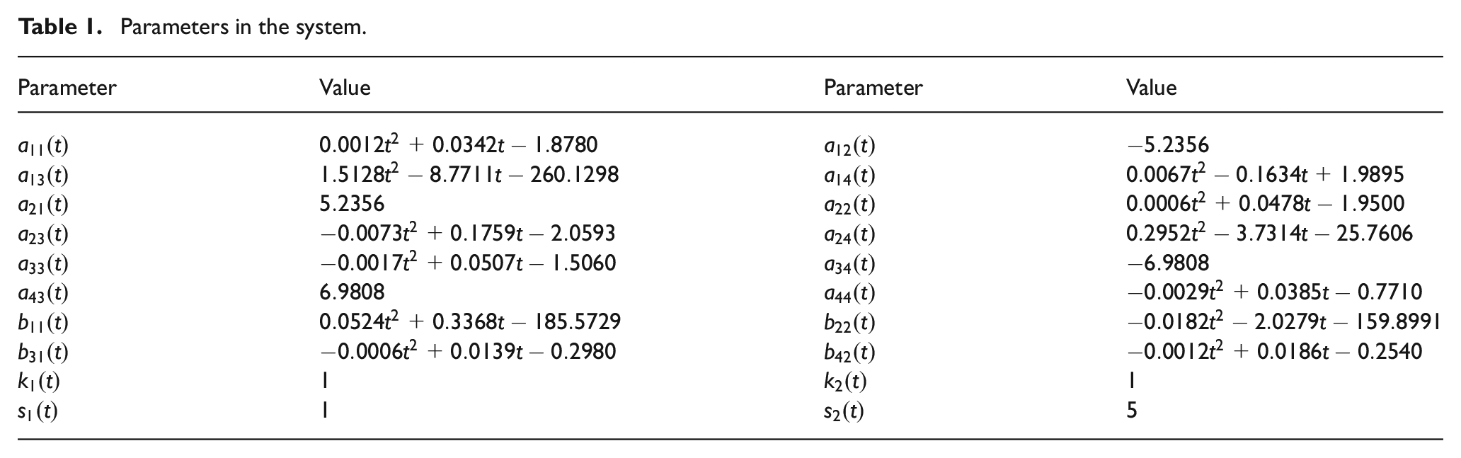
The data fitted to the correlation matrices of the BTT system and observer are shown in Table 1.

Table 1.

Parameters in the system.

Parameter	Value	Parameter	Value
$a_{11} (t)$	$0.0012 t^{2} + 0.0342 t - 1.8780$	$a_{12} (t)$	$- 5.2356$
$a_{13} (t)$	$1.5128 t^{2} - 8.7711 t - 260.1298$	$a_{14} (t)$	$0.0067 t^{2} - 0.1634 t + 1.9895$
$a_{21} (t)$	$5.2356$	$a_{22} (t)$	$0.0006 t^{2} + 0.0478 t - 1.9500$
$a_{23} (t)$	$- 0.0073 t^{2} + 0.1759 t - 2.0593$	$a_{24} (t)$	$0.2952 t^{2} - 3.7314 t - 25.7606$
$a_{33} (t)$	$- 0.0017 t^{2} + 0.0507 t - 1.5060$	$a_{34} (t)$	$- 6.9808$
$a_{43} (t)$	$6.9808$	$a_{44} (t)$	$- 0.0029 t^{2} + 0.0385 t - 0.7710$
$b_{11} (t)$	$0.0524 t^{2} + 0.3368 t - 185.5729$	$b_{22} (t)$	$- 0.0182 t^{2} - 2.0279 t - 159.8991$
$b_{31} (t)$	$- 0.0006 t^{2} + 0.0139 t - 0.2980$	$b_{42} (t)$	$- 0.0012 t^{2} + 0.0186 t - 0.2540$
$k_{1} (t)$	$1$	$k_{2} (t)$	$1$
$s_{1} (t)$	$1$	$s_{2} (t)$	$5$

Then following parametric results can be drawn from equation (40)

\begin{matrix} {\begin{matrix} H (t) = [\begin{matrix} h_{11} (t) & h_{12} (t) \\ h_{21} (t) & h_{22} (t) \end{matrix}] \\ L (t) = [\begin{matrix} l_{11} (t) & l_{12} (t) \\ l_{21} (t) & l_{22} (t) \end{matrix}] \\ R (t) = {[\begin{matrix} 0.0012 t^{2} + 0.0342 t + 6.3576 \\ 0.0006 t^{2} + 0.0478 t + 50.8144 \end{matrix}]}^{T} \end{matrix} \end{matrix}

(42)

where

\begin{matrix} {\begin{matrix} h_{11} (t) = 0.0000174 t^{4} + 0.0011552 t^{3} + 3.08877928 t^{2} \\ - 44.25062596 t - 567.5322452 \\ h_{12} (t) = - 0.00003528 t^{4} - 0.0022638 t^{3} + 0.534461 t^{2} \\ + 104.8704442 t + 7751.778546 \\ h_{21} (t) = - 0.00000072 t^{4} - 0.00000384 t^{3} - 0.02514182 t^{2} \\ - 0.9757442 t + 199.052632 \\ h_{22} (t) = 0.0000072 t^{4} + 0.000462 t^{3} - 0.09848408 t^{2} \\ - 21.56627016 t - 1579.754158 \end{matrix} \end{matrix}

and

\begin{matrix} {\begin{matrix} l_{11} (t) = 0.00001224 t^{4} - 0.0000162 t^{3} + 9.208894 t^{2} \\ - 35.09775036 t + 2256.133644 \\ l_{12} (t) = - 0.00008526 t^{4} - 0.00566048 t^{3} - 15.02243538 t^{2} \\ + 212.9039726 t + 2112.208162 \\ l_{21} (t) = - 0.00000204 t^{4} + 0.0000027 t^{3} - 1.54006026 t^{2} \\ + 5.1586086 t - 628.1076725 \\ l_{22} (t) = 0.0000174 t^{4} + 0.0011552 t^{3} + 3.08877928 t^{2} \\ - 44.25062596 t - 567.5322452 \end{matrix} \end{matrix}

Furthermore, we can get other coefficient matrices of observer (10) as

\begin{matrix} {\begin{matrix} T^{+} (t) = [\begin{matrix} 6 & 0 \\ 0 & 10 \\ - 0.0072 t^{2} - 0.2052 t + 219.8124 & 0 \\ 0.0294 t^{2} + 2.3422 t + 327.8636 & 0 \end{matrix}] \\ T^{-} (t) = [\begin{matrix} 0 & 1 \\ 49 & 0 \\ 0 & - 0.0012 t^{2} - 0.0342 t + 45.234 \\ 0 & 0.478 t + 0.006 t^{2} + 75.7356 \end{matrix}] \\ S^{+} (t) = [\begin{matrix} 1 & 5 \end{matrix}], S^{-} (t) = [\begin{matrix} 0 & 0 \end{matrix}] \end{matrix} \end{matrix}

(43)

and

{\begin{matrix} | L (t) | = [\begin{matrix} l_{11} (t) & l_{12} (t) \\ - l_{21} (t) & - l_{22} (t) \end{matrix}] \\ | R (t) | = {[\begin{matrix} 0.0012 t^{2} + 0.0342 t + 6.3576 \\ 0.0006 t^{2} + 0.0478 t + 50.8144 \end{matrix}]}^{T} \end{matrix}

(44)

Consider the initial values as

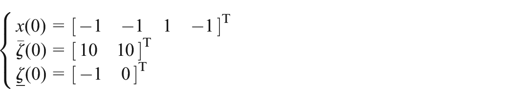
{\begin{matrix} x (0) = {[\begin{matrix} - 1 & - 1 & 1 & - 1 \end{matrix}]}^{T} \\ \bar{ζ} (0) = {[\begin{matrix} 10 & 10 \end{matrix}]}^{T} \\ \underline{ζ} (0) = {[\begin{matrix} - 1 & 0 \end{matrix}]}^{T} \end{matrix}

without loss of generality, choose the control input as $u_{1} (t) = u_{2} (t) = 0$ , $0 \leq t \leq 15$ . The simulation results are plotted in Figure 3 –5.

Figure 3.

System responses before and after disturbance.

Figure 4.

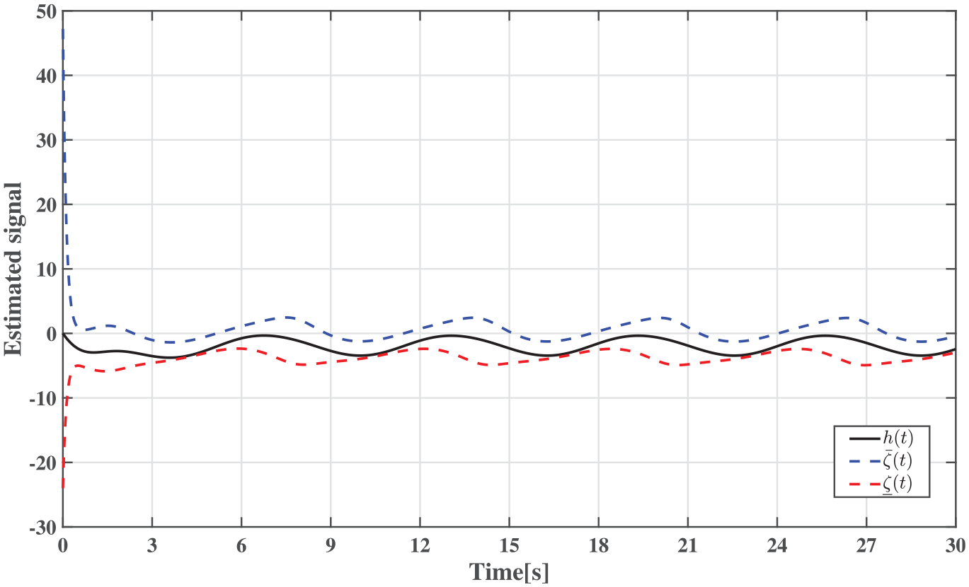
Observation effect of the designed observer.

Figure 5.

Output interval.

Figure 3 shows the functional state responses of the system before and after the disturbance, which are denoted by $h^{-} (t)$ and $h (t)$ , respectively, indicating that the additional disturbance does have some effect on the original system. Figure 4 shows the functional signal to be observed and the responses of the designed observer, while Figure 5 shows the output interval defined as $e (t) = \bar{ζ} (t) - \underline{ζ} (t)$ . It can be seen that bounds provided by the proposed observer can well realize interval estimation of the functional signal, which verifies the effectiveness of this parametric design.

Conclusion

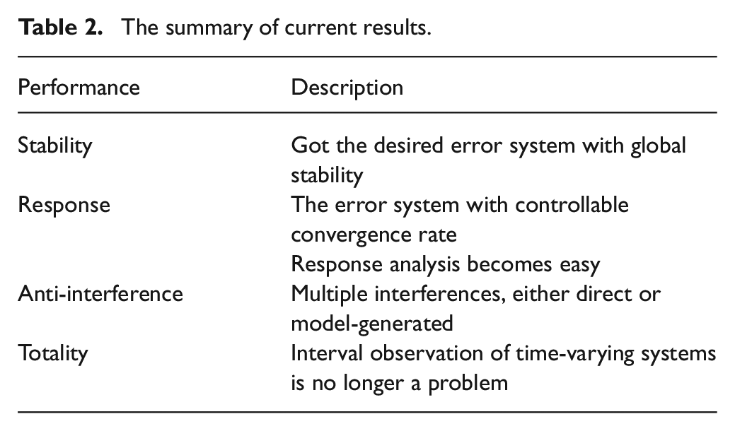
In this research, we propose a parameterized design method to address the functional interval estimation of LTV systems with additional but bounded disturbances. First, for estimating bounds of the functional states, an interval observer is designed and the corresponding existence conditions are given. Next, based on the solution of GSE, we provide an effective algorithm for calculating the gain matrices, and a parameterized design process. Finally, the effectiveness of this method is verified by the simulation experiment of a numerical example and the BTT aircraft control system. The current work is summarized in Table 2.

Table 2.

The summary of current results.

Performance	Description
Stability	Got the desired error system with global stability
Response	The error system with controllable convergence rate
	Response analysis becomes easy
Anti-interference	Multiple interferences, either direct or model-generated
Totality	Interval observation of time-varying systems is no longer a problem

For the next study, we can extend the idea of this paper to other systems such as descriptor time-varying and time-delay to solve more interval estimation problem.

Footnotes

Declaration of conflicting interests

The author(s) declared no potential conflicts of interest with respect to the research, authorship, and/or publication of this article.

Funding

The author(s) disclosed receipt of the following financial support for the research, authorship, and/or publication of this article: This work was supported by the Science Center Program of the National Natural Science Foundation of China under Grant No. 62188101 and also by the Major Program of National Natural Science Foundation of China under Grant Nos 61690210 and 61690212.

ORCID iD

Da-Ke Gu

Yin-Dong Liu

References

Ahlem

Harouna

Saida

, et al. (2016) Design of a functional adaptive observer for bilinear delayed systems. IFAC: Papers Online 49(10): 25–30.

Bezzaoucha

Voos

Darouach

(2018) A new polytopic approach for the unknown input functional observer design. International Journal of Control 91(3): 658–677.

Duan

(2014) Generalized Sylvester Equations: Unified Parametric Solutions. Boca Raton, FL: CRC Press.

Duan

Wang

(2005) Multi-model switching control and its application to BTT missile design. Acta Aeronautica et Astronautica Sinica 26(2): 144–147.

Efimov

Perruquetti

Raïssi

, et al. (2013a) Interval observers for time-varying discrete-time systems. IEEE Transactions on Automatic Control 58(12): 3218–3224.

Efimov

Polyakov

Richard

(2015) Interval observer design for estimation and control of time-delay descriptor systems. European Journal of Control 23: 26–35.

Efimov

Raïssi

Zolghadri

(2013b) Control of nonlinear and LPV systems: Interval observer-based framework. IEEE Transactions on Automatic Control 58(3): 773–778.

Efimov

Raïssi

Chebotarev

, et al. (2013c) Interval state observer for nonlinear time varying systems. Automatica 49(1): 200–205.

Gouzé

Rapaport

Hadj-Sadok

(2000) Interval observers for uncertain biological systems. Ecological Modelling 133(1): 45–56.

10.

Wang

(2022) A high-order fully actuated system approach for a class of nonlinear systems. Journal of Systems Science and Complexity 35(2): 714–730.

11.

Liu

Duan

(2019) A parametric method of linear functional observers for linear time-varying systems. International Journal of Control Automation and Systems 17(3): 647–656.

12.

Liu

(2022a) Parametric design of functional interval observer for time-delay systems with additive disturbances. Circuits, Systems, and Signal Processing 41(5): 2614–2635.

13.

Liu

Yang

(2020) Linear function observers for linear time-varying systems with time-delay: A parametric approach. IEEE Access 8: 19398–19405.

14.

Sun

Liu

(2021a) Parametric design to reduced-order functional observer for linear time-varying systems. Measurement and Control 54(7–8): 1186–1198.

15.

Sun

Liu

(2022b) Parametric design of functional observer for second-order linear time-varying systems. Asian Journal of Control. Epub ahead of print 4 May. DOI: 10.1002/asjc.2843.

16.

Sun

Liu

(2022c) Reduced-order functional observers for descriptor linear time-invariant systems: A parametric method. International Journal of Adaptive Control and Signal Processing 36(3): 562–578.

17.

Wang

Liu

(2021b) Parametric approach of partial eigenstructure assignment for high-order linear systems via proportional plus derivative state feedback. AIMS Mathematics 6(10): 11139–11166.

18.

Wang

Liu

, et al. (2022d) Parametric design of reduced-order functional observers for linear time-varying delay systems. Measurement and Control. Epub ahead of print 9 August. DOI: 10.1177/00202940221104481.

19.

Xie

(2016) Control of non-linear switched systems with average dwell time: Interval observer-based framework. IET Control Theory & Applications 10(1): 10–16.

20.

Huong

Trinh

(2016) New state transformations of time-delay systems with multiple delays and their applications to state observer design. Journal of the Franklin Institute 353(14): 3487–3523.

21.

Huong

Huynh

Trinh

(2020) Interval functional observers for time-delay systems with additive disturbances. International Journal of Adaptive Control and Signal Processing 34(9): 1281–1293.

22.

Xia

, et al. (2019) Remote nonlinear state estimation with stochastic event-triggered sensor schedule. IEEE Transactions on Cybernetics 49(3): 734–745.

23.

Duan

(2017) Observer design for a class of linear time-varying systems. In: Proceedings of the 2017 36th Chinese control conference (CCC), Dalian, China, 26–28 July, pp. 116–121. New York: IEEE.

24.

Liu

Xie

Khan

, et al. (2020) Finite-time functional interval observer for linear systems with uncertainties. IET Control Theory & Applications 14(18): 2868–2878.

25.

Liu

Xie

Zhang

, et al. (2022) Time-dependent Luenberger-type interval observer design for uncertain time-varying systems. International Journal of Robust and Nonlinear Control 32(7): 4195–4213.

26.

Luenberger

(1966) Observers for multivariable systems. IEEE Transactions on Automatic Control 11(2): 190–197.

27.

Mazenc

Dinh

Niculescu

(2014) Interval observers for discrete-time systems. International Journal of Robust and Nonlinear Control 24(17): 2867–2890.

28.

Moisan

Bernard

Gouz

(2007) Near optimal interval observers bundle for uncertain bioreactors. In: Proceedings of the 2007 European control conference (ECC), Kos, 2–5 July, pp. 5115–5122. New York: IEEE.

29.

Raïssi

Efimov

Zolghadri

(2012) Interval state estimation for a class of nonlinear systems. IEEE Transactions on Automatic Control 57(1): 260–265.

30.

Shen

Huo

Cao

, et al. (2019) Generalized state estimation for Markovian coupled networks under round-robin protocol and redundant channels. IEEE Transactions on Cybernetics 49(4): 1292–1301.

31.

Smith

(1995) Mathematical Surveys and Monographs: Monotone Dynamical Systems: An Introduction to the Theory of Competitive and Cooperative Systems, vol. 41. Providence, RI: American Mathematical Society.

32.

Thabet

REH

Raissi

Combastel

, et al. (2014) An effective method to interval observer design for time-varying systems. Automatica 50(10): 2677–2684.

33.

Volkov

Demyanov

(2016) Functional observer design using linear matrix inequalities. Optoelectronics, Instrumentation and Data Processing 52(4): 334–340.

34.

Wang

Lim

Shen

(2018) Interval observer design for uncertain discrete-time linear systems. Systems & Control Letters 116: 41–46.

35.

Puig

Ocampo-Martinez

, et al. (2014) Actuator-fault detection and isolation based on set-theoretic approaches. Journal of Process Control 24(6): 947–956.

36.

Puig

Ocampo-Martinez

, et al. (2015) Set-theoretic methods in robust detection and isolation of sensor faults. International Journal of Systems Science 46(13): 2317–2334.

37.

Zhang

Cong

Ling

, et al. (2019) An efficient and fast quantum state estimator with sparse disturbance. IEEE Transactions on Cybernetics 49(7): 2546–2555.

38.

Zhang

Yin

Zhang

(2011) An improved adaptive observer design for a class of linear time-varying systems. In: Proceedings of the 2011 Chinese control and decision conference (CCDC), Mianyang, China, 23–25 May, pp. 1395–1398. New York: IEEE.

39.

Zheng

Zhang

Yan

(2016) Distributed

H^{\infty}

filtering for active semi-vehicle suspension systems through network with limited capacity. In: Proceedings of the 2016 35th Chinese control conference (CCC), Chengdu, China, 27–29 July, pp. 7352–7357. New York: IEEE.