






Abstract
Process monitoring technology can help make the right decisions in manufacturing, but the complexity and scale of modern process industry processes render process monitoring difficult. Existing data-driven process monitoring methods utilize abundant monitoring data that are accumulated in industrial processes, but nonlinearity, high coupling, noise effects, and other problems continuously appear in process industry monitoring data. This study proposes a process monitoring method based on variational autoencoder and long short-term memory techniques. The method reconstructs the monitoring data by learning their distribution and time series characteristics under the controlled state, and then it monitors the state of the manufacturing process in real time by calculating the statistics. Evaluation is conducted using the Tennessee Eastman process case verification and experimental comparison method. Then, the proposed method is compared with the centralized process via principal component analysis and kernel principal component analysis. The results show that the proposed method can more significantly improve the effect of fault detection in distributed system process monitoring compared with the traditional method, and it has a better process monitoring effect.
Introduction
Process monitoring technology is an important means of ensuring manufacturing process safety and product quality stability, and it has been widely used in industrial production practice (Tang et al., 2022). For decades, process monitoring has gradually developed into a research field involving mathematical statistics, signal processing, automatic control, machine learning, and other disciplines, even evolving into many branches, such as analytical models, expert systems, and data analysis (Chan et al., 2005; Rong et al., 2021; Wang et al., 2007). Nowadays, owing to the development of modern process industry technology, massive process data can be recorded, which greatly promotes the development of data-driven process monitoring technology. Among the data-driven methods, the development of multivariate statistical process monitoring methods is relatively mature and has a wider impact. Moreover, artificial intelligence technologies, such as machine learning, are gradually introduced into the research of process monitoring and have achieved good results.
In the previous studies for process monitoring, the multivariate statistics methods in processing high-dimensional data are often used to analyze complex process monitoring variables. Among them, principal component analysis (PCA) (Tang et al., 2022) and partial least squares (PLS) (Wang et al., 2007) can realize the change of data dimension mapping while preserving the key information in the data to the maximum extent. After that, the manufacturing process could be effectively characterized (Sabahno et al., 2021). For example, PCA is used to determine the controlled state of a monitoring process and to diagnose process variables in uncontrolled states (Fuentes-Garcia et al., 2018). There are also studies that apply multiple linear regression (Luo et al., 2016) and variables-based weighted Fisher discriminant analysis (Lu and Yan, 2022) to process monitoring to realize online monitoring and visual process monitoring. However, most changes of the variables in actual industrial processes are nonlinear, which is particularly prominent as the process industry is becoming complex (Wu et al., 2021). Therefore, kernel functions are introduced into process monitoring to ensure that linear statistical analysis methods meet practical requirements (Apsemidis et al., 2020). Some studies have analyzed the correlation between monitoring variables and introduced kernel functions into PCA (Jiang and Yan, 2018) and PLS (Harrou et al., 2015) methods to distinguish linear and nonlinear relationships between variables. Liu et al. (2019) proposed a highly robust process monitoring method based on kernel-independent component analysis, which could focus on the components related to system performance, to highlight the performance-related change in the modeling. In addition, the local model-based approach is applied to process monitoring models because it can represent nonlinear space into different linear subspaces to overcome nonlinear problems. However, the applicability of this method is poor (Zhong et al., 2021). In recent years, machine learning, especially deep learning, offers powerful data processing capabilities; it can process complex high-dimensional space by training large numbers of monitoring variable data, allowing them to more suitably address the needs of the process industry, including process monitoring tasks. Considering the similarities and differences of nonlinear process operation modes, a process monitoring method based on stacked autoencoder (AE) was proposed (Meiners et al., 2021; Wang et al., 2021a). In order to improve the ability to identify the characteristics of process monitoring variables, Li et al. (2021) proposed an embedded dictionary learning method with AEs for nonlinear industrial process monitoring, which is robust to samples. In general, machine learning method has superior performance in modeling, and its data-driven characteristics are in line with the industrial characteristics of the big data. However, the existing statistical methods and machine learning methods still have great difficulties in the face of the requirements of distributed monitoring data.
The manufacturing process of the modern industry is highly complex and widely distributed, but the process conditions are even more complicated and affect one another. Furthermore, the monitoring method based on global modeling is difficult to apply in these situations (Cao et al., 2021). Many researchers have proposed distributed monitoring scenarios where centralized manufacturing can be decomposed based on empirical knowledge or data characteristics. Liu et al. (2014a) developed a parallel decentralized distributed monitoring scheme that can simultaneously locate faults in input and output variables. Han et al. (2018) proposed a multi-model PCA distributed process monitoring method for unstable industrial processes and used the case of steel rolling to verify the effectiveness of their approach to reduce the false alarm rate (FAR). Li et al. (2020) divided them into different blocks according to the mutual information of monitoring variables. A case involving a time-varying process was used to select the method with the best online monitoring effect. Wu et al. (2022) proposed a knowledge- and data-driven large-scale distributed process monitoring method that could fully utilize the spatiotemporal information of monitored variables to accurately detect process faults.
However, the partitioning of local subblocks in these distributed process monitoring methods relies heavily on prior process knowledge (Zhu et al., 2018). But, in the actual distributed production process, the characteristics of dynamic manufacturing process changing in real time cannot be captured in real time. Therefore, Xu et al. (2017) proposed a dynamic PCA model to dynamically capture time-varying features in distributed manufacturing processes through an enhanced data matrix. Jiang and Jiang (2021) proposed a variable Bayes probability latent variable (VBPLV) method by analyzing the autocorrelation and interrelationship between process data and quality data in the distributed process. With the development of data-driven distributed monitoring models, Liu et al. (2014b) and Jiang et al. (2019) both established a distributed monitoring framework based on variational Bayesian principal component analysis (VBPCA), which improved the stability of the framework in processing missing data. However, Jiang et al. (2019) improved the method and proposed a VBPCA-CCA (CCA, Canonical Correlation Analysis) distributed detection method based on VBPCA. VBPCA is used to process the missing value of data, and CCA is used to analyze the correlation between variables to realize distributed monitoring. However, it is difficult to obtain specific correlations between variables in complex industrial systems by relying solely on VBPCA and CCA. Although many studies have attempted to further strengthen the distributed process monitoring method in the process industry and to some extent achieved results. However, there are still some problems in distributed process monitoring, such as nonlinear, high coupling, and low adaptability. Among them, nonlinear and coupling problems of monitoring data hinder most distributed process monitoring tasks (Jiang et al., 2020).
Aiming to overcome the above problems, this paper proposes a process monitoring model combining the long short-term memory (LSTM) network and variational autoencoder (VAE), hereafter referred to as VAE-LSTM, based on distributed scenarios. The construction of the VAE-LSTM model is driven by process monitoring data and its relevant parameters are also determined through monitoring data, and does not rely on the operation principle or experience knowledge of the process industry. VAE model describes the potential space of data by means of probability generation, while LSTM units are used to replace simple neurons in the encoder and decoder, which can mine the timing features of manufacturing process data in the reconstruction task. The combination of the two can effectively help to optimize the defects of feature extraction of the VAE model and further improve the accuracy of encoding and decoding by using the timing information existing in the monitoring variables. Therefore, the VAE-LSTM model can better adapt to complex monitoring data requirements and various process industry characteristics than traditional process monitoring methods and better handle nonlinearity and coupling of monitoring data in the industrial manufacturing process. In this paper, we first select the required monitoring variables and determine the monitoring points according to the processes adopted in the process industry. Then we highlight the practical significance of each monitoring variable, combine statistical calculation and knowledge and experience to determine the correlation between the monitoring variables, and use the community network algorithm to further explore their correlation. Finally, we divide the correlation into different sub-units, construct a process monitoring sub-model based on VAE-LSTM for each sub-unit as a means of implementing process monitoring tasks, and perform feature extraction and dimensionality reduction processing on the monitoring variables in each sub-unit. The overall process monitoring model, which is based on the final process monitoring results, can help to make manufacturing decisions.
The rest of this paper is organized as follows. Section “Preliminaries” introduces the VAE model process monitoring method. Section “VAE-LSTM process monitoring based on distributed scenarios” introduces the VAE-LSTM process monitoring scheme based on distributed scenarios. Section “Case study” presents the performance of the method through numerical examples and the application of the Tennessee Eastman (TE) process. Section “Conclusions and outlooks” gives the conclusions and suggestions of this research.
Preliminaries
Variational autoencoder
VAE is a deep generative model that is often used to solve complex data construction problems. It has the ability to generate reconstructed data according to the distribution of the original data (Nazábal et al., 2020). VAE can also be regarded as a special or evolved AE, with its model structure similar to that of the traditional AE model. Figure 1 shows the two main parts of the VAE model, namely, the encoder and decoder (Samandari Masooleh et al., 2022). The encoder maps the high-dimensional input data into low-dimensional hidden variables, while the decoder maps the low-dimensional hidden variables into high-dimensional data. This study adopts the VAE model to realize the reconstruction task of complex monitoring data.

VAE model structure.
The VAE model is a generative model with hidden variables. Hidden variables refer to those variables that cannot be directly observed and are generally obtained by inferring the samples of the observable variables. Furthermore, hidden variables have a certain influence on the output of observable variables in the model (Xu and Cai, 2022). This study takes the monitored variables in the manufacturing process as the input data, and variational inference is performed on them to generate the probability distributions of latent variables, which can be described as several independent drivers affecting the quality of the manufacturing process (e.g., variable operations, specific processes, etc.). In this manner, the original data can be reconstructed as much as possible and ultimately used as the output, thus realizing the aforementioned reconstruction task of complex process monitoring data.
In the process monitoring task, the observable N monitoring variable sets are
The latent variable is an important influencing factor of the monitoring variable, i.e., the monitoring variable sets
The K-L divergence likelihood function
The maximum likelihood estimation, which is intractable in the computational process, turns into a variational low-bound problem that can optimize the likelihood estimation. When
The expected error term
Long short-term memory network
The LSTM algorithm adds a cell structure similar to a “processor” to judge the value of current information; this technique is often used to process time-related data sequences and solve the long-term and short-term data in the data set (Landi et al., 2021). In industrial processes, a strong dynamic temporal relationship usually exists between the process data sequences. LSTM uses the aforementioned feature to process and learn the relationship of the monitored variables.
The structure of LSTM is similar to that of RNN, as both models are composed of a series of neural units. The improvement is that each cell consists of three special structures: forget gate, input gate, and output gate (Wang et al., 2021b). For each monitoring variable, a certain relationship exists between the values of the sample points before and after the time series. Through these special “gate” structures, LSTM can better realize the inputting, selection, and outputting of monitoring variable data and address the time series correlations between variables during monitoring. The structure of the LSTM network is shown in Figure 2.

LSTM network structure.

“Gate” structure of the LSTM network.

Schematic diagram of the sub-unit division results.
As shown in Figure 3, the input monitoring variable data first reaches the forget gate, and then this forget gate decides whether to discard part of the information in the input data, i.e., the influence of the forward monitoring sample point data on the current sample point data is ignored. The gate reads
The input gate is responsible for processing the input monitoring variable data
Upon completing the forget gate and input gate functions, the state of the current cell structure is updated from
The final output gate determines the output feature data
VAE-LSTM process monitoring based on distributed scenarios
This study proposes a process monitoring method based on distributed scenarios, focusing on solving the actual needs of the current manufacturing process; thus, it is also suitable for solving the complex correlation between the high-dimensional characteristics of the process system and the process variables. The method mainly includes three steps. First, the process monitoring variables are divided into different sub-units. Second, process monitoring is performed by independently modeling each sub-unit. Finally, the characteristics of the monitoring variables in the sub-units are extracted, processed, and transmitted. Once the process monitoring model reaches the process monitoring center, it integrates the monitoring variables of the sub-units and judges the controlled situation of the overall process.
Sub-unit division based on the Girvan–Newman algorithm
Sub-unit division is a key step in process monitoring in distributed scenarios. Here, we use the Girvan–Newman (GN) algorithm for sub-unit division. The method combines specific physical characteristics of monitoring variables and is driven by data to automatically output sub-unit division results. The GN algorithm is an important community structure discovery algorithm. It utilizes the characteristics of strong intra-community correlation and weak inter-community correlation in the social network, adopts the splitting idea to gradually delete the edges in the network, and divides the network into multiple communities. In process monitoring, we can regard monitoring variables as nodes in a network and sub-units as communities, thereby dividing a complex industrial process into multiple communities related to the operational variables.
First, we construct an undirected graph network for the GN algorithm based on the correlation between the monitored variables. All process-related monitoring variables are used as nodes in an undirected graph. In this study, mathematical methods are used to calculate the correlation coefficient between the monitoring variables. Two monitoring variable nodes with strong correlation are connected by edges, and the judgment can be combined with the actual situation when setting the threshold. On the basis, an undirected graph network composed of monitoring variables can be obtained to simultaneously reflect the correlation between the different monitoring variables in terms of physical meaning and observation data.
The GN algorithm is used to divide the sub-units according to the edge betweenness in the monitoring variable network, in which the edge betweenness of each edge refers to the number of shortest paths through the edge in the entire network. The definition of edge betweenness can help to establish the importance of the edge in the network. For instance, if an edge connects different sub-units, then the shortest path between two points located on the different sub-units will pass through this edge with high probability, and the edge betweenness of the edge will increase. Similarly, if an edge is only located inside the sub-unit, then only the shortest path between some nodes inside the sub-unit will pass through the edge, and the edge betweenness of the edge will be reduced. When removing the edge with the largest edge betweenness in the network, the probability by which different sub-units will be separated is high. Furthermore, the GN algorithm calculates the shortest path in the network based on this idea of determining the edge betweenness of each edge and finally deletes the edge with the largest edge betweenness. The abovementioned operations are repeated iteratively until certain conditions are met, including the expected number of sub-units. The calculation of edge betweenness is shown in equation (11). In the formula,
In the process of dividing the sub-units in the GN algorithm, the number of sub-units and the optimal dividing result cannot be determined. In response to this problem, Newman proposed modularity
Modularity
Process monitoring based on VAE-LSTM
A process monitoring model based on VAE-LSTM is constructed in this study. As opposed to models or knowledge-driven methods, the proposed model is driven by process monitoring data. In other words, the model construction process does not need to be based on the operating principles or empirical knowledge of the process industry; rather, it is determined by monitoring data. By using relevant parameters in the model, the combined VAE and LSTM model can achieve accurate dynamic modeling in the reconstruction task of time series-related data. The model uses LSTM units embedded in the VAE model for building encoders and decoders to learn the dependence of monitoring variables in time series, realize the mutual mapping between monitoring variables and latent variables, and calculate the monitoring variable data for reconstruction. Monitoring statistics are used to determine whether the monitored state is under control. The modeling steps can be summarized as process variable data reconstruction, monitoring statistics calculation, and controlled state determination, as shown in Figure 5. It should be noted that Figure 5 includes local monitoring results and global monitoring results in process monitoring. In the actual manufacturing process, when the local monitoring results are inconsistent with the global monitoring results, the local monitoring results can timely send an alarm to the fault location and describe the fault situation in more detail. The specific experimental analysis can be seen in Figure 5.

Application steps of the process monitoring model based on VAE-LSTM.
Due to the distributed process monitoring, the number of monitored variables in each sub-unit is less, and the correlation is stronger. The process monitoring model is easier to learn and explore the internal relationship between variables, so as to achieve a better monitoring effect. The monitoring process within the sub-unit can be divided into two aspects: offline construction model and online process monitoring. In this study, offline data and online data are used jointly. The specific data division can be seen in Section “Monitoring case based on the TE process.” It should be noted that, during the process monitoring in the sub-unit, if the local production process is found to be in an uncontrolled state due to abnormal faults, the process monitoring model can directly issue an uncontrolled state warning to the sub-unit. In addition, sub-unit process monitoring is the description of local information. Each sub-unit will carry out feature extraction and dimension reduction processing of its own monitoring variables and input them into the process monitoring center. The process monitoring model here will collect all sub-unit information to monitor the whole process.
In VAE-LSTM, the LSTM units are used to replace simple neurons in the encoder and decoder. The temporal information in the monitoring variables can then be used to improve the encoding and decoding tasks. In the encoder, the monitoring variable set

Application steps of the process monitoring model based on VAE-LSTM.
In the process monitoring task, we design corresponding monitoring indicators to measure whether the current state is under control. Then, in accordance with the goal of obtaining the reconstructed data
The
After calculating the monitoring indicators
This study takes the process industry as the research object. Two evaluation indicators, namely, fault detection rate (FDR) and FAR, are used to evaluate the application effect of the process monitoring model. FDR refers to the ratio of the samples whose monitoring indicators exceed the control limit to the total samples, while FAR refers to the ratio of the samples whose monitoring indicators exceed the control limit to the controlled samples. We also use fault delay as a basis for evaluation. Fault delay refers to the time difference from the occurrence of the fault to the fault being identified. As the fault occurrence time in this study is uniform, it can also be represented by the sample points where the fault has been identified. In particular, the formulas are shown in equations (17) and equations (18)
In these equations,
Case study
The performance of the proposed process monitoring model was evaluated by simulation experiments using two cases. The first case was based on numerical simulation, whereas the other case was based on TE process simulation (Downs and Vogel, 1993). We selected two traditional data-driven process monitoring models (PCA and KPCA [Kernel Principal Component Analysis]) and compared them with the proposed model. Between the two models, PCA can reduce the processing difficulty of monitoring variables by mapping changes in the data space dimension. As PCA does not need to build a mechanism model, it has a strong versatility and is even utilized as an important benchmark model in the process monitoring field. Meanwhile, KPCA introduces the kernel method by using the concept of higher dimensions. In this method, spatial mapping changes can be better applied to solve nonlinear problems and thus can meet the need of production work. KCPA has also become an important method for process monitoring.
Numerical example
In this section, a simple nonlinear system is constructed via numerical simulation to verify the effectiveness of the proposed method. The specific description of the system is given by
where
The above process represents the normal operation data of a system in a controlled state. According to the above formula, all controlled state data samples required for case verification can be generated, including a total of 500 monitoring samples. Besides, we select different faults to generate the fault samples in the system in an uncontrolled state. The specific fault settings can be described as follows:
Fault 1: Inject fault at the 100th training sample,
Fault 2: Inject fault at the 100th training sample,
Fault 3: Inject fault at the 100th training sample,
Fault 4: Inject fault at the 100th training sample,
Fault 5: Inject fault at the 100th training sample,
In the VAE-LSTM model, the input dimension is defined as 52 × 20, which means that each input is a set of complete operation sequences, namely, 52 groups of operation variables. The input dimension is defined according to the size of the input data set itself. Meanwhile, the training and optimization determine that the loss value of batch size will stabilize the fastest in a round of 20. That is, 20 operation sequences are used as a batch in each round for model training. Each iteration cycle of the model is 100 times. The input of the encoder is Linear(in, Hidden) and the output is Linear(Hidden, out), and Sigmoid is used to activate the encoder layer for forward propagation. Among them, the initial VAE-LSTM layer is the 3-dimensional input of Linear(480 × 52,256), which is converted into a 2-dimensional vector of Linear(256,128) and finally connected with the LSTM network. The network layer is determined to be a three-layer LSTM network through training optimization, as shown in Figure 7(a). The blue curve represents the average value in the whole training process. The VAE-LSTM model uses the Sigmoid function to activate. The encoder part uses permute function for latitude transposition, and the decoder part is similar to the encoder part. The final control is carried out through KL divergence, and the optimization results are output. Figure 7(b) shows the network iterative optimization values under different numbers of potential variables. The number of potential variables of the model is finally determined to be 5, and the confidence level is set to 0.99. After 300 rounds of iterative model training, the learning rate of the model training process gradually decreases and tends to be stable, as shown in Figure 8.

Optimization process curve of the VAE-LSTM model. (a) LSTM layers. (b) VAE latent variables.

The curves of VAE-LSTM training process loss value.
We use the controlled state data samples as the training set and the fault data samples as the test set through the case study method to verify the effect of the proposed process monitoring model. We construct process monitoring models based on VAE-LSTM, PCA, KPCA, VAE, LSTM, KECA (Kernel Entropy Component Analysis), DPCA (Dynamic Principal Component Analysis), VBPCA, and VBPLV, respectively. The monitoring results of these nine models are shown in Table 1. Table 1 shows that VAE-LSTM has a higher FDR than the single PCA, KPCA, VAE, and LSTM process monitoring models, and the monitoring statistics of
Process monitoring via numerical simulation: Monitoring results of nine models.
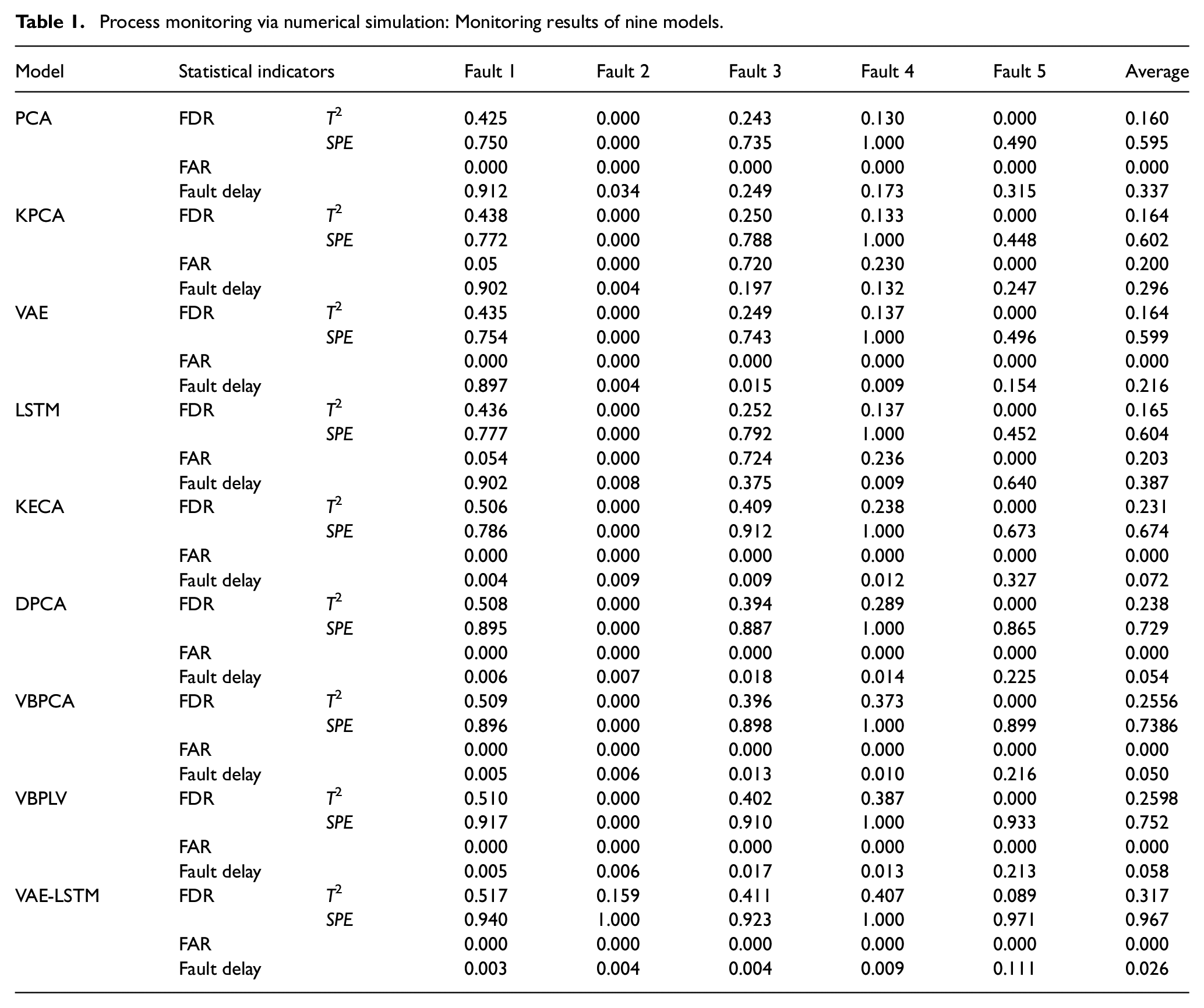
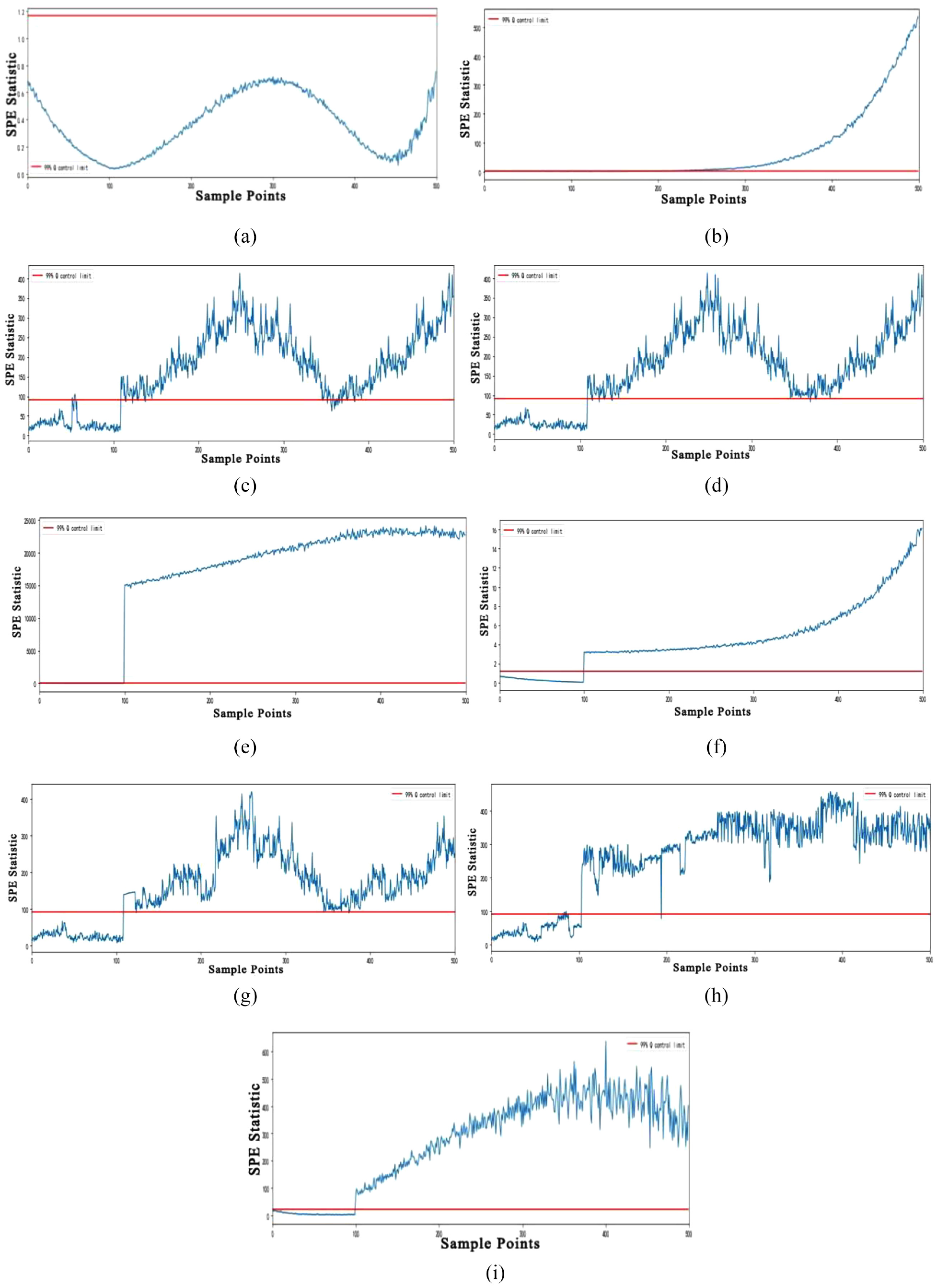
Fault 1 is a slow-growing fault, and its impact on the system becomes more and more significant over time. In the actual manufacturing process, such faults should be discovered as early as possible to avoid greater losses. As can be seen from the process monitoring results in Figure 9, the monitoring statistics trends of the nine models are basically similar, all of which indicate that the abnormal influence brought by the fault is constantly increasing. The VAE-LSTM model starts to recognize abnormal states at the 125th sample point, while PCA, KPCA, VAE, LSTM, KECA, DPCA, VBPCA, and VBPLV only recognize abnormal states at the 200th, 191th, 362th, 365th, 195th, 189th, 216th, and 291th sample points, respectively. The VAE-LSTM model takes into account the timing characteristics of the monitored variables, so it has better performance in the aspect of fault delay. However, the KECA model sends out a fault warning signal when no fault is added, and an obvious step change occurs when the 100th sample is added to the fault. This is because the time sequence characteristics of the manufacturing process were not considered in the construction of the vector and feature space of the KECA model, leading to step warning of fault occurrence. On the contrary, the VAE-LSTM model has a more stable and accurate performance for monitoring slow growth faults. VAE and LSTM models have low detection performance for slow-increasing faults. Corresponding to the fault delay shown in Table 1, the mean fault delay time consumption is 0.216 and 0.387, respectively. It can be seen from Figure 9 that, compared with the VBPCA model, the sensitivity of the VBPLV model to the fault delay is also corresponding to the results in Table 1. Since fault 1 is a slow drift fault, the fault missing value in this fault has little influence on the fault. Therefore, the use of the variable Bayesian formula to repair missing values may change the slow-growing fault trend. As shown in Figure 9(e), the final monitoring results of the VBPCA method fluctuate greatly, which does not conform to the fault characteristics of slow growth. Although the VBPLV model has better fault monitoring results than VBPCA, its sensitivity to faults is lower than that of VBPCA due to a lack of analysis on time series characteristics, which corresponds to the first fault alarm sample position (VBPCA: 216th and VBPLV: 291th), and the alarm time of VBPLV is later. In addition, the average fault delay time consumption of the VBPCA and VBPLV models in Table 1 is 0.050 and 0.058, respectively, which need to be improved compared with VAE-LSTM distributed process monitoring model.

SPE statistic monitoring curve of fault 1 in the numerical simulation case. (a) PCA. (b) KPCA. (c) VAE. (d) LSTM. (e) KECA. (f) DPCA. (g) VBPCA. (h) VBPLV. (i) VAE-LSTM.
SPE statistic monitoring curve of fault 2 in the numerical simulation case. (a) PCA. (b) KPCA. (c) VAE. (d) LSTM. (e) KECA. (f) DPCA. (g) VBPCA. (h) VBPLV. (i) VAE-LSTM.
From a mathematical point of view, both faults 2 and 3 change the individual coefficients in the formula. Since what is changed in fault 2 is the corresponding coefficient of the function, it can be seen from the properties of the trigonometric function that its influence is small, and it can belong to the category of minor faults, which are often difficult to detect and identify. Taking fault 2 as an example, according to the process monitoring results in Figure 7, it can be seen that the monitoring curve based on PCA and KPCA models fluctuates but does not exceed the threshold, that is, the model cannot effectively identify the fault. The VAE-LSTM model can detect the significant change of
The aforementioned analysis indicates that, compared with FDR and FAR, the VAE-LSTM process monitoring model is better than PCA, KPCA, VAE, LSTM, KECA, DPCA, VBPCA, and VBPLV process monitoring models that can effectively carry out process monitoring tasks for nonlinear systems. At the same time, it also has a good sensitivity to various types of faults and has a good performance in fault delay, FDR, and other aspects. However, when faced with a fault situation with the influence of time characteristics, the accuracy of fault monitoring of KECA and DPCA models is reduced. It can be seen from the experimental results that the process monitoring model based on VAE-LSTM can be applied to nonlinear process industry scenarios. The model monitors the current system running state from the perspective of distribution characteristics and timing characteristics of monitoring data, and can effectively process monitoring timing samples. As the VAE-LSTM model needs to go through multiple iterations, the computational complexity is greater in the training process compared with the centralized process monitoring method. However, the centralized process monitoring model needs to calculate the distance between points in advance, and it requires too much memory and overhead to calculate the eigenmatrix of big data, which will inevitably require greater space-time complexity and affect the speed and accuracy of the algorithm. When the VAE-LSTM model is trained and entered into the testing and monitoring process, the computing time consumption is the shortest, and the average time consumption is 0.0042 seconds. VAE (0.0098 seconds) and LSTM (0.0099 seconds) are of the same order of magnitude as VAE-LSTM. The time consumption of other centralized monitoring models is relatively large: PCA (0.3276 seconds), KPCA (0.01078 seconds), KECA (0.0134 seconds), and DPCA (0.0149 seconds). Therefore, compared with the centralized process monitoring model, VAE-LSTM model can better satisfy the fault response in the actual manufacturing process.
Monitoring case based on the TE process
The TE process is an open simulation platform developed by the U.S.-based Eastman Chemical Company for the actual chemical industrial reaction process (Huang et al., 2020). The data generated by this platform have nonlinear, time-varying, and strong coupling characteristics, and they are widely used in process monitoring and fault diagnostic test tasks of complex industrial processes; consequently, the TE process has become a classic benchmark that is widely recognized by the academic community (Li and Yang, 2021).
In this study, the simulation data of the TE process are used as an example to verify the performance of the process monitoring method in the distributed scenario. Then, the centralized process monitoring method is used to compare the process monitoring effect in the distributed scenario. The TE process is a simulation modeling of the real chemical reaction process involving eight chemical components: A, C, D, and E are gaseous reactants, B is an inert gas, G and H are liquid products, and F is the liquid by-product. The TE process flow is shown in Figure 11. To better verify the application effect of the distributed scenario, we select all 52 variables in the TE process as the monitoring variables.
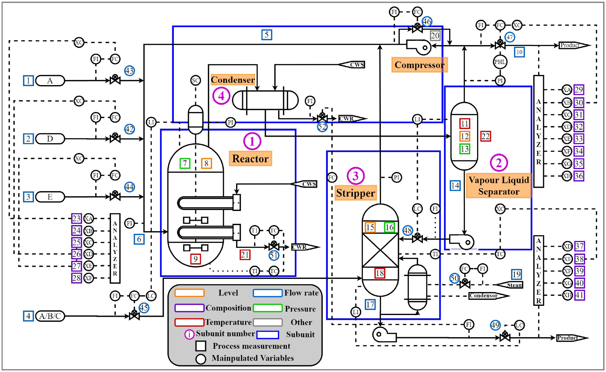
TE process flow.
The sub-unit division is initially performed. Fifty-two different process monitoring variables are involved in the TE process. The number of variables is large, and their relationships are complex; subsequently, they need to be divided into different sub-units. Using the sub-unit division method of the GN algorithm, we construct the monitoring variable network
The monitoring data under the control state are used as the object for calculating the correlation coefficient between the monitoring variables. In this experiment, the Spearman correlation coefficient is selected as the basis. The calculation results are shown in Figure 12. Positive numbers represent positive correlations, whereas negative numbers represent negative correlations. The depth of the color represents the strength of the correlation. The 52 monitoring variables are numbered accordingly from 1 to 52. The correlation among the 52 variables is relatively complex and has no obvious regularity. Take the XMEAS (6) reactor feed rate as an example. This monitoring variable has a prominent correlation with XMEAS (12) and XMEAS (15), which represent the liquid level of the gas–liquid separator and the level of the stripper, but they are located in different reaction production units. Consequently, the nodes they represent are connected to determine the hidden correlations.
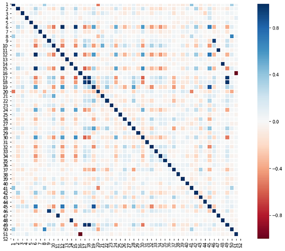
Calculation results of the correlation coefficients among monitoring variables.
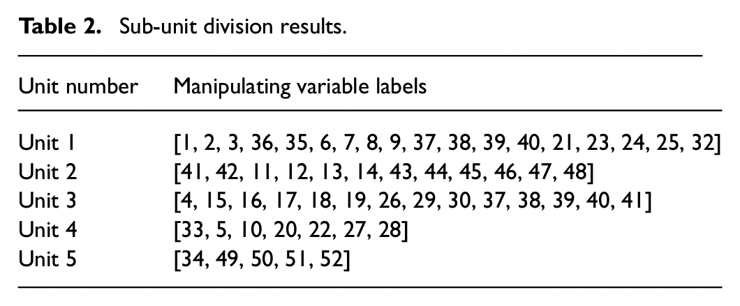
At this point, the monitoring variable network has been constructed. The nodes in the network represent different monitoring variables, and the edges represent the correlation between two connected nodes. The GN algorithm is used to iteratively calculate the modularity size and sub-unit division results of the undirected graph network. As shown in Figure 13, when the number of sub-units is 5, the modularity can reach the maximum value; thus, the optimal number of sub-units for the monitoring variable network is also selected as 5. The sub-unit division results are shown in Table 2, and the visualization results are shown in Figure 14. For convenience, XMEAS (1) to XMEAS (41) are numbered 1–41 in the chart, while XMV (1) to XMV (11) are numbered 42–52.
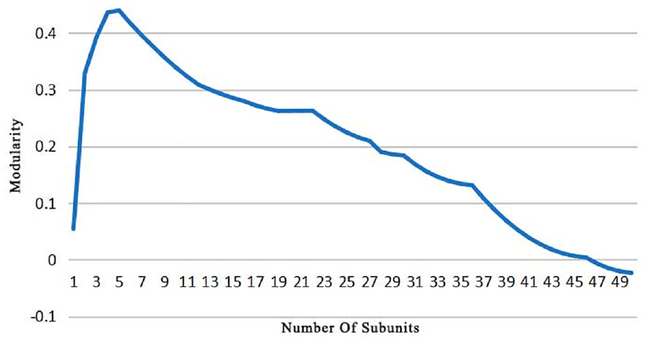
Modularity changes corresponding to different numbers of the sub-units.
Sub-unit division results.
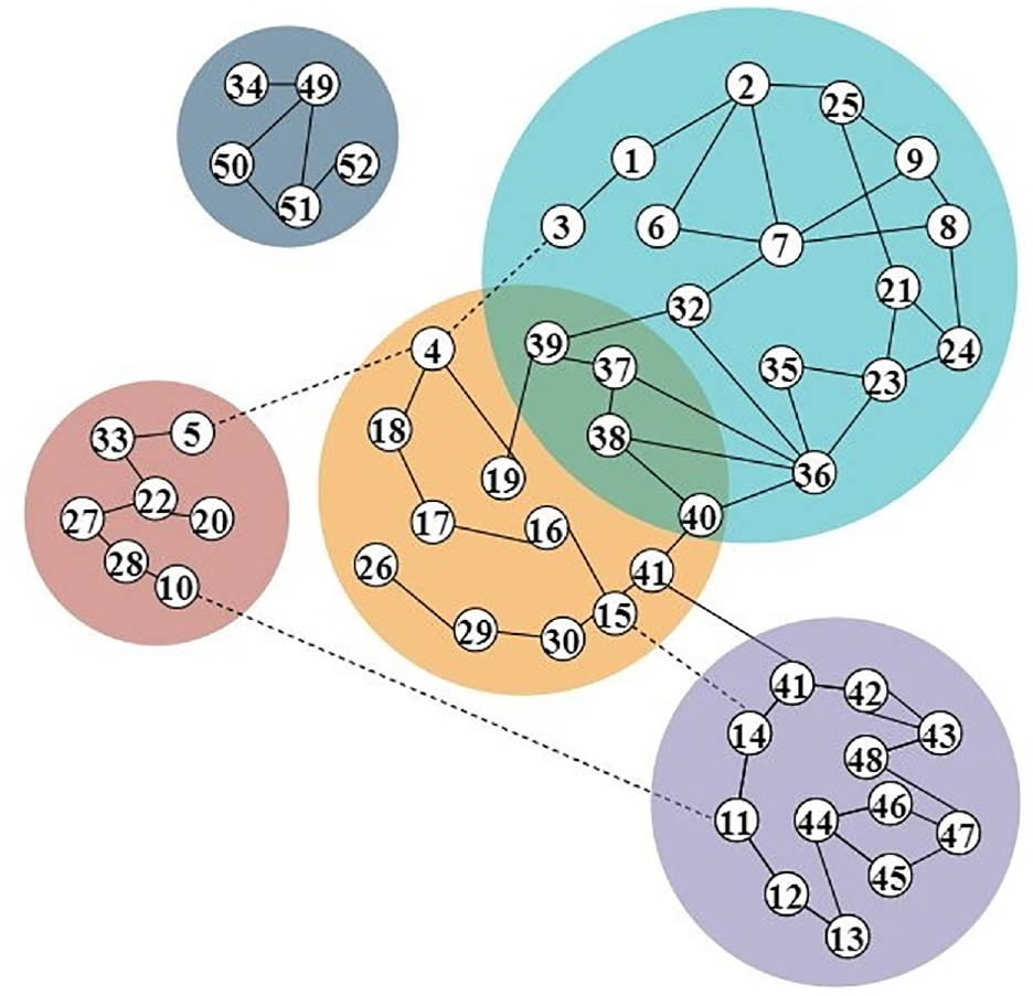
Visualization of the sub-unit division results.
At this point, the monitoring task of the TE process has been decomposed into five different sub-unit process monitoring tasks, which are denoted as
This study focuses on the application effect of the process monitoring model in the overall manufacturing monitoring. In the offline modeling process, the study adopts the offline simulation data set for model training and takes the normal data set of the TE process with dimension 480 × 52 and the data set with fault latitude 960 × 52 as the input data set. In the process of online modeling, since the component measurement variables in process industry are not available for online real-time measurement (such as XMEAS (23) component A, XMEAS (24) component B, etc.), this study selects the control variables that can be obtained online in the manufacturing system of process industry. For example, XMV (1) D feed amount, XMV (2) E feed amount (11), and process measurement variables such as XMEAS (7) reactor pressure and XMEAS (9) reactor temperature (22) as monitoring variables, a total of 33. Some typical faults of the TE process have been specifically analyzed to evaluate the application effect of the process monitoring model based on distributed scenarios.
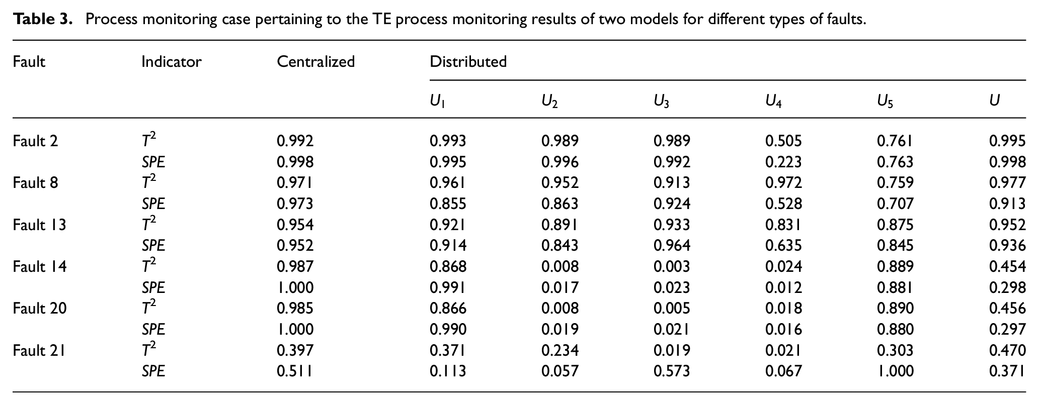
Fault 2 is a step-type fault. Under the condition that the feed flow ratio of reactants A and C in feed stream 4 is the same, the content of component B changes abruptly. Fault 2 will cause the feedstock to flow to the stripper, causing a step change in production unit A during operation. The monitoring results of the two models are shown in Table 3. Take the
Process monitoring case pertaining to the TE process monitoring results of two models for different types of faults.
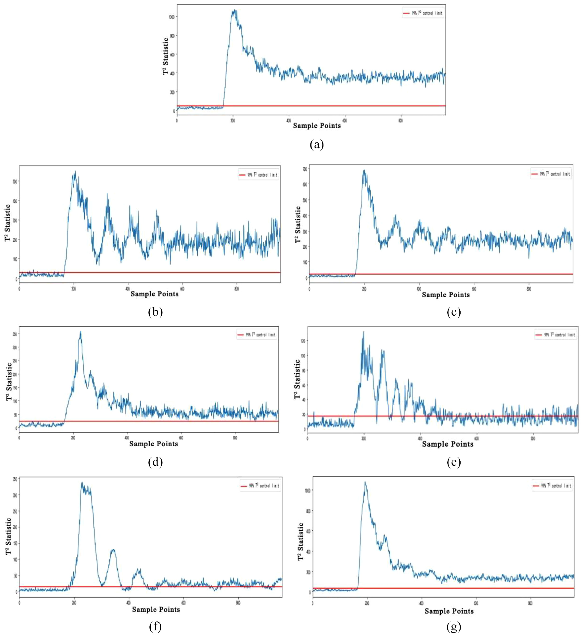
T 2 statistic monitoring curves of different models for fault 2. (a) Centralized model. (b) U1. (c) U2. (d) U3. (e) U4. (f) U5. (g) U.
Fault 8 is a random variable-type fault. The compositional ratios of reactants A, B, and C in feed stream 4 change randomly, further resulting in random fault changes in the operating conditions of the stripper production unit. The monitoring results of the two models are also shown in Table 3. Take again the
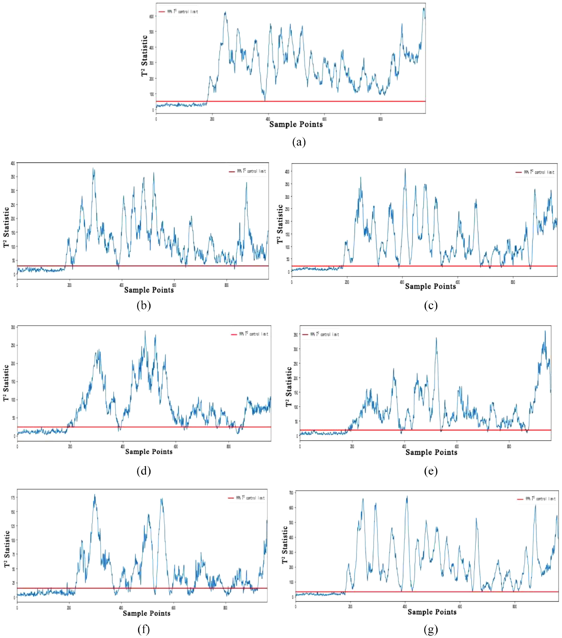
T 2 statistic monitoring curves of different models for fault 8. (a) Centralized model. (b) U1. (c) U2. (d) U3. (e) U4. (f) U5. (g) U.
Table 3 also shows the monitoring results of other fault types. The distributed process monitoring model proposed in this study can maintain the performance of the centralized monitoring model while maintaining the performance of the divided sub-units. The process monitoring model has unique advantages in terms of local description, fault diagnosis, and low computational complexity, among others.
The obtainment of the abovementioned results can be summarized as follows. First, this study builds the undirected graph network of the monitoring variables by considering their physical meanings and the computational correlations among them, and the GN algorithm is used to divide the monitoring variable network to obtain the different sub-units. Furthermore, by considering both empirical knowledge and mathematical laws, the sub-unit division results are guaranteed to be more reliable, and the problems of lack of interpretability and difficulty in practical application caused by the single method are simultaneously avoided. Second, on the basis of the comparison with the centralized process monitoring model, the correlations among sub-units often lead to higher FDRs and lower fault delay under the condition of partial local faults. Nonetheless, the distributed process monitoring model can provide a specific local description. Third, by observing the process monitoring results of the different sub-units, we can more clearly explain their respective impact on the current manufacturing process, especially since different sub-units have varying sensitivities to the same fault. Through distributed process monitoring, we can provide a basis for subsequent tasks, such as fault diagnosis and positioning, according to the response of the sub-units to the faults, which is more advantageous than simply relying on the centralized process monitoring model. More importantly, the division of the sub-units is a simple task, suggesting reduced computational complexity of the sub-unit process monitoring model, and it also facilitates rapid model construction and calculation. In the actual manufacturing process of the process industry, compared with transmitting massive monitoring data to the same location, the use of a distributed monitoring model can better improve the speed of data transmission and processing while reducing the cost of process monitoring. In the current situation of the process industry which has become increasingly complex, the process monitoring model based on distributed scenarios is more suitable for multi-unit, distributed, and other complex process industry scenarios, suggesting highly relevant application and practical value.
Conclusion and outlooks
In this study, a process monitoring method based on distributed scenarios is proposed in view of addressing the nonlinear, time series, noise, and other characteristics of process industry data. A monitoring variable network is constructed by considering the monitoring variables and their mathematical correlations. Then, the network is divided into sub-units by using the GN algorithm. Finally, a model for performing process monitoring tasks is built independently for each sub-unit. The model sub-unit division scheme can effectively solve the problems of high correlation and complex monitoring variable dimensions, and it can be feasibly implemented in practical applications. Case studies based on the TE process are also conducted. The monitoring effect of the proposed model is investigated by comparing it with a centralized process monitoring model. The results show that the process monitoring model based on the distributed scenario can obtain FDR and FAR that are similar to those of the centralized scheme, but significant improvements in these two measures can be guaranteed for some partial faults. The process monitoring model based on distributed scenarios also has unique advantages. For instance, the proposed scheme can provide a more specific local description of faults and provide a basis for subsequent tasks, such as fault diagnosis and location sensing. At the same time, it can reduce the complexity of model construction and data monitoring. Furthermore, the costs and delays of processing and transmission have practical implications. The proposed method can be applied to more complex process industry scenarios, such as multi-unit and distributed scenarios, among others. Furthermore, it can solve problems involving many monitoring points, large amounts of data, strong coupling, and delays across different units in actual scenarios. Our method is more in line with the development needs of the process industry.
In future work, typical fault characteristics will be considered to improve the sensitivity of the model to small faults, allowing it to become more adaptable to different fault types. For complex production scenarios, future work also needs to consider multi-fault scenarios based on time or production units. These multi-faults cannot be simply superimposed or canceled in the monitoring variables given their mutual influences. These effects need to be determined through further research.
Footnotes
Acknowledgements
The authors thank all the participants in the experiment and the professors for their advice. The authors would like to thank the anonymous reviewers for their valuable suggestions and constructive comments.
Declaration of conflicting interests
The author(s) declared no potential conflicts of interest with respect to the research, authorship, and/or publication of this article.
Funding
The author(s) disclosed receipt of the following financial support for the research, authorship, and/or publication of this article: The work reported herein was supported by Shaanxi Province Natural Science Foundation Research Project (2023-JC-YB-615).
