A new fault component selection strategy based on statistical detection for slewing bearing weak signal de-noising

Abstract

Slewing bearing is a critical transmission component in large-size construction machinery due to its low-speed and heavy-load conditions. Fault prognostics and health management of slewing bearing are crucial for ensuring their high availability and profitable operation. However, the presence of background noise in construction machinery signals restricts the applicability of existing signal processing approaches in prognostics and health management. To address this challenge, a novel signal de-noising method is proposed based on adaptive decomposition, along with a new strategy for recognizing fault components using statistic detection through kernel principal component analysis (KPCA). First, robust local mean decomposition is utilized to adaptively decompose the fault and normal vibration signal over the entire service life. Then, product functions (PFs) decomposed by fault and normal vibration signal are used for KPCA anomaly detection. Finally, the fault PFs are reconstructed to obtain the de-noised signal. The effectiveness of the proposed method is validated through the use of both simulated and experimental vibration signals obtained from a slewing-bearing life-cycle test. The results illustrate that the proposed method has superior de-noising capability and decomposition efficiency, making it an effective signal preprocessing technique for prognostics and health management.

Keywords

Slewing bearing signal de-noising fault component recognition robust local mean decomposition kernel principal component analysis

Introduction

Slewing bearings are critical transmission components in various industrial equipment such as tunnel boring machines and wind turbines. Due to the lack of necessary monitoring device, small undetected faults can potentially lead to catastrophic failures, including major accidents, which have a serious impact on the safe operation of industry. Therefore, effective prognostics and health management approaches are essential for extending the service life of slewing bearings and improving the operation efficiency of industrial equipment. Prognostics and health management of rotating machinery can be mainly divided into four steps: (a) data acquisition; (b) feature extraction; (c) health indicator construction; and (d) remaining useful life prediction (Lee et al., 2014). Among these four steps, the most challenging step is feature extraction as vibration signals collected from slewing bearings are often contaminated with significant amounts of working noise. Therefore, effective signal de-noising for subsequent steps is challenging but crucial.

Similar to small-size high-speed bearing, rotating components such as inner ring, outer ring, cages, and balls are inevitable parts of slewing bearing (Amasorrain et al., 2003). The vibration signals obtained from slewing bearings are mixed signals from multiple blind sources, and the fault defect-related signal is often submerged by background noise due to the low energy of fault information and the low revolving speed of slewing bearing, which is typically lower than 10r/min. Therefore, separating fault-related component from background noise is a critical first step before processing vibration signals from slewing bearings (Pan et al., 2022a). Generally, signal processing methods need to know a priori information about the fault frequency bands related to damage for the rings, balls, and other components (Jia et al., 2017). Wavelet and its derivative algorithm is one of the most commonly used methods in bearing vibration signal processing (Imane et al., 2021; Li et al., 2019; Pan et al., 2022b). However, how to choose wavelet basis function limits the application of wavelet de-noising (Graps, 1995). Empirical mode decomposition (EMD) is an effective technique for self-adaptive signal decomposition, capable of decomposing a signal into different intrinsic mode functions (IMFs) with distinct frequency bands (Huang et al., 1998). However, the mode mixing problem is a major drawback of EMD (Tang et al., 2012). As an improvement of EMD, ensemble empirical mode decomposition (EEMD) adds Gaussian white noise into the process of EMD and eliminates the signal intermittence (Wu and Huang, 2011). Although EEMD eliminates the issue of mode mixing in EMD, it introduces Gaussian white noise to the original signal multiple times, resulting in a significant reconstruction error in signal decomposition (Zheng et al., 2014). Moreover, the repeated execution of EMD increases the computational burden. To overcome the drawback, Smith (2005) proposed a new self-adaptive signal decomposition method called local mean decomposition (LMD), which effectively reduces the number of iterations and improve the decomposition speed. Besides, robust LMD (RLMD) can optimize the algorithm structure and strengthen the decomposition performance compared with traditional LMD (Liu et al., 2017). To facilitate the processing of highly nonlinear and non-stationary signals such as slewing bearing vibration signals, we adopt RLMD for signal-noise separation, which holds even greater promise than other techniques.

After adaptive signal decomposition, fault component selection can be carried out to separate the fault-related component from the background noise and de-noise the signal. The selection strategy for the decomposed component can be broadly categorized into three types: (a) Correlation-based selection: This strategy involves calculating the correlation between the fault signal and each of its decomposed components. The component with the highest correlation coefficient is then selected as the fault-related component (Kumar et al., 2019; Ma et al., 2018; Yao et al., 2021). (b) Characteristics-based selection: This strategy involves analyzing the characteristics of decomposed components, such as kurtosis (Li et al., 2018; Zhao et al., 2021), power (Han et al., 2018), permutation entropy (Li et al., 2018), and so on. The component with the highest characteristic is then selected as the fault-related component. (c) Combination-based selection: This strategy combines correlation-based and characteristics-based selection strategies to quantify the fault defect-related degree of the decomposed components. For instance, a combination of correlation coefficient and kurtosis criteria is utilized to measure the degree of fault defect-related information contained in decomposed components (Cheng et al., 2019; Fu et al., 2018; Wang et al., 2019). However, these selection strategies are vulnerable to background noise that is unrelated to the fault or normal operation of the system. Considering the low-speed heavy-load operation characteristics of slewing bearing, whether the above strategies are applicable to slewing bearings deserves further research (Caesarendra and Tjahjowidodo, 2017; Pan et al., 2021). With the advantage of multiscale nature, Bakshi (1998) put forward the multiscale principal component analysis (PCA) method. Multiscale PCA utilizes wavelet coefficients at each scale, which are subjected to PCA to extract components that exhibit distinct signatures for their standard conditions, which change in response to the occurrence of faults. However, the main limitation of wavelet analysis is the need to select an appropriate wavelet basis function (Graps, 1995). To solve this shortcoming, Feng et al. (2015) combined EEMD with PCA, which is utilized to decompose vibration signals and select the fault components across the entire life-cycle signals. Even though PCA is widely used for fault diagnosis, it suffers from a major limitation of being a linear method and may pass over some useful nonlinear features (Žvokelj et al., 2010). To overcome this deficiency, Žvokelj et al. (2011) proposed a de-noising and diagnosis approach for large-size bearings using an EEMD-kernel PCA (KPCA) method. The methodology in general resembles the recently developed EEMD-PCA scheme (Žvokelj et al., 2010) but differs from it in using KPCA instead of linear PCA, allowing it to handle linear as well as nonlinear correlations among process variables. However, EEMD inevitably suffers from large reconstruction errors. Therefore, based on the advantages of RLMD and KPCA, a weak signal de-noising method is proposed using RLMD-KPCA for slewing bearing. Hence, KPCA is employed to select the fault product function (PF) component. Therefore, the proposed signal de-noising method named RLMD-KPCA exploits the merits of RLMD to handle blind source mixed signals and the benefits of KPCA to recognize abnormal information.

To address the aforementioned issues, a novel signal de-noising methodology for large-size low-speed slewing bearings is proposed using RLMD-KPCA. RLMD is a robust signal decomposition method that can effectively separate the vibration signals of a slewing bearing into different PFs. Then, KPCA is applied to fault component recognition of slewing bearing. The methodology is validated using experimental data collected from a slewing-bearing life-cycle test. The results show that the proposed method achieves high accuracy in signal de-noising, making it more suitable for slewing bearing preprocessing analysis.

The remainder of this paper is organized as follows: Section “Methodology” outlines the systematic methodology of signal de-noising. The signal adaptive decomposition and statistical detection methods are proposed for the enhancement of signal de-noising. Section “Proposed de-noising model based on RLMD-KPCA” shows the process of the proposed method based on RLMD-KPCA. In section “Numerical verification and experimental analysis,” the proposed method is validated on simulated as well as life-cycle test dataset. The conclusions and recommendations for future research are presented in section “Conclusions and future works.”

Methodology

Signal adaptive decomposition using robust RLMD

EEMD adds white noise to the original signal and repeats the decomposition process multiple times to reduce mode mixing. However, this process introduces additional noise and leads to large reconstruction errors. In addition, the repeated execution of EMD increases the computational cost, making it impractical for some applications. As an improvement, LMD can effectively reduce the number of iterations and shorten the computation time. LMD can decompose the non-stationary modulation signal into several PFs, and each PF is directly calculated by an envelope signal and a pure frequency modulation (FM) signal. The process of LMD can be summarized as follows:

(i) Find out all the local extremum n_i of raw signal x(t), and calculate the local mean m_i and envelope estimation a_i of adjacent extremum as follows

m_{i} = \frac{n_{i} + n_{i + 1}}{2}

(1)

a_{i} = \frac{| n_{i} - n_{i + 1} |}{2}

(2)

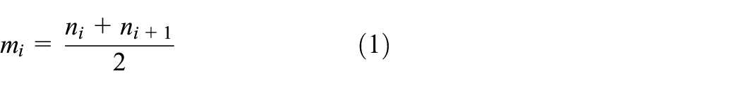
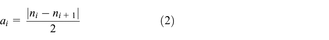
(ii) Utilize straight lines to connect all local mean m_i and envelope estimation a_i, and obtain the corresponding function m₁₁(t) and a₁₁(t) using the moving average method.

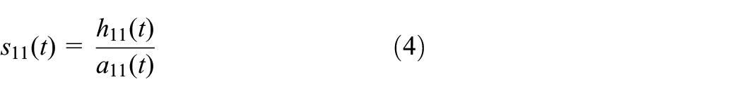
(iii) Get h₁₁(t) by separating the local mean function m₁₁(t) from x(t), and divide h₁₁(t) by a₁₁(t) to get the demodulated signal s₁₁(t)

h_{11} (t) = x (t) - m_{11} (t)

(3)

s_{11} (t) = \frac{h_{11} (t)}{a_{11} (t)}

(4)

(iv) Envelope estimation function a₁₂(t) can be obtained through repeating the above process for s₁₁(t). When s_1n(t) becomes a pure FM signal, the repeat implementation stops.

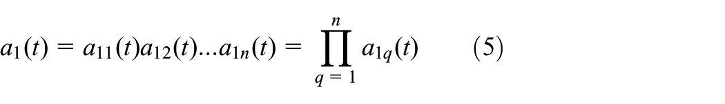
(v) Obtain the envelope signal a₁(t) by taking the product of all local envelope estimation functions

a_{1} (t) = a_{11} (t) a_{12} (t) . . . a_{1 n} (t) = Π_{q = 1}^{n} a_{1 q} (t)

(5)

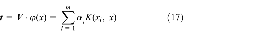
where the first PF₁ is obtained by taking the product of a₁(t) and FM signal

{PF}_{1} (t) = a_{1} (t) s_{1 n} (t)

(6)

(vi) Get the new signal u₁(t) as follows

u_{1} (t) = x (t) - {PF}_{1} (t)

(7)

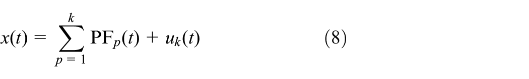
(vii) Repeat the circulation implementation of Steps (i)–(vi). The calculation of LMD ends when u_k(t) is a monotonic function or contains no oscillations. Then, output the decomposed PFs and residual signal u_k(t)

x (t) = \sum_{p = 1}^{k} {PF}_{p} (t) + u_{k} (t)

(8)

As an improvement over LMD, RLMD can effectively improve three aspects, namely, boundary condition, envelope estimation, and sifting stopping criterion, to reduce the mode mixing problem and increase the accuracy of signal decomposition. The updated process of RLMD can be summarized as follows (Liu et al., 2017): (a) Boundary conditions (Step (i) of LMD): Mirror extension algorithm (Rilling et al., 2003) is used to determine the symmetrical points at the left and right ends of the signal. After that, m_i and a_i can be calculated. (b) Envelope estimation (Step (ii) of LMD): Based on the statistics theory, a statistical method is utilized to define a reasonable fixed subset size for accurate envelope estimation automatically. Afterward, the moving average algorithm, regarded as the smoothing algorithm, is employed for envelope estimation for m₁₁(t) and a₁₁(t). (c) Sifting stopping criterion (Step (iv) of LMD): The objective function within the repeat implementation, used to describe the zero-baseline envelope signal, is presented as

f = RMS (z (t)) + EK (z (t))

(9)

where $z (t) = a (t) - 1$ , that is, the zero-baseline envelope signal

RMS (z (t)) = \sqrt{\frac{1}{N_{s}} \sum_{t = 1}^{N_{s}} z {(t)}^{2}}

(10)

EK = \frac{\frac{1}{N_{s}} \sum_{t = 1}^{N_{s}} {[z (t) - \bar{z}]}^{4}}{{(\frac{1}{N_{s}} \sum_{t = 1}^{N_{s}} {[z (t) - \bar{z}]}^{2})}^{2}} - 3

(11)

The sifting stopping criterion of the objective function is defined as below: a_ij(t) represents the smoothed local magnitude computed from the jth iteration in the sifting process of the ith PF. The objective function value f_ij in each iteration can be determined by referring to its definition in equation (9). The proposed sifting stopping criterion is based on the evaluation of f_ij, f_ij₊₁, and f_ij₊₂, which are obtained from three consecutive iterations. If f_ij₊₁> f_ij and f_ij₊₂>f_ij₊₁, the sifting process terminates and returns the corresponding results from the (j–1)th iteration. Otherwise, the sifting process continues until the maximum number of iterations allowed in each sifting process is reached.

Statistical detection using KPCA

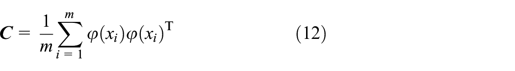
The essence of PCA is to map a multi-dimensional data matrix to the principal component subspace and residual subspace and utilize a small amount of principal component information to represent all variables. Hence, the principal components are not correlated with each other. However, PCA suffers from linear property, abandoning the information of higher-order statistics. As a nonlinear extension of PCA, Schölkopf et al. (1998) proposed KPCA by adding a kernel function to PCA. The data X is mapped into high-dimensional space F by kernel function φ(·), and perform PCA in high-dimensional space. It can transform the data from being linearly inseparable in low-dimensional space to linearly separable in high-dimensional space.

The covariance matrix C in the space F and its vector analysis can be calculated by

C = \frac{1}{m} \sum_{i = 1}^{m} φ (x_{i}) φ {(x_{i})}^{T}

(12)

λ V = CV

(13)

where λ is the eigenvalue and V is the eigenvector. The inner product of each high-dimensional space sample φ(x_i) and equation (13) is as follows

λ [φ (x_{k}) \cdot V] = [φ (x_{k}) \cdot CV]

(14)

where the eigenvector V of covariance matrix C can be expressed by φ(x_i) linearly

V = \sum_{j = 1}^{m} α_{j} φ (x_{j})

(15)

where α_j is the correlation coefficient. Substituting equation (15) into equation (14) gives the following result

λ \sum_{j = 1}^{m} α_{j} [φ (x_{k}) \cdot φ (x_{j})] = \frac{1}{m} \sum_{j = 1}^{m} α_{j} [φ (x_{k}) \cdot \sum_{i = 1}^{m} φ (x_{i})] [φ (x_{i}) \cdot φ (x_{j})]

(16)

Defining an $m \times m$ -dimensional kernel matrix K , that is, K_ij = (φ(x_i)·φ(x_j)) and K is a symmetric matrix, then equation (16) can be expressed as $m λ α = K α$ . So, the eigenvector V of eigenvalue covariance C can be obtained from the eigenvector $α$ of matrix K , that is, the principal component direction of the variable sample matrix X in the high-dimensional feature space F . The projection of mapping data on the eigenvector V of space F is presented by

t = V \cdot φ (x) = \sum_{i = 1}^{m} α_{i} K (x_{i}, x)

(17)

In addition to feature dimensionality reduction, KPCA has been widely used to recognize abnormal equipment conditions. The main principle behind this technique is to determine whether a signal is normal or abnormal by comparing its projection onto the principal component subspace and residual subspace with a given threshold. There are two commonly used statistical detection methods Hotelling T² statistics and squared prediction error (SPE). This study takes KPCA-SPE statistics as an indicator to recognize abnormal condition as KPCA-SPE statistics is more sensitive than Hotelling T² statistics in detecting abnormal condition

SPE = ‖ φ (x), φ_{k} (x) ‖^{2} = \sum_{i = 1}^{n} t_{i}^{2} - \sum_{i = 1}^{k} t_{i}^{2}

(18)

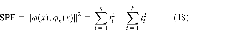
where t_i is the projection in the ith feature direction, n is the number of feature dimension, and k is the number of principle components. The threshold of SPE is given by

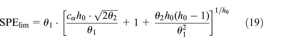
{SPE}_{lim} = θ_{1} \cdot {[\frac{c_{α} h_{0} \cdot \sqrt{2 θ_{2}}}{θ_{1}} + 1 + \frac{θ_{2} h_{0} (h_{0} - 1)}{θ_{1}^{2}}]}^{1 / h_{0}}

(19)

where c_α is the Gauss distribution of confidence level (1–α)%. h₀ = 1–2θ₁θ₃/3θ₂² and θ_d =∑ ⁿ _j = k+1λ_j^d (d = 1, 2, 3). λ_j is the jth eigenvalue of the covariance matrix of X.

The implementation procedure for recognizing abnormalities is listed step by step as follows, incorporating the SPE statistic:

(i) Establish the baseline model of SPE using normal data, and calculate the SPE threshold, as known as SPE_lim.

(ii) Map the online monitoring data onto the baseline model to obtain SPE. Then, compare it with the threshold SPE_lim to judge whether the online condition is abnormal or not. If SPE > SPE_lim, it indicates an abnormal online condition, otherwise, the opposite holds normal.

Proposed de-noising model based on RLMD-KPCA

Following signal decomposition using the RLMD, PFs can be obtained and arranged in descending order of frequency, where PFs with higher frequency contain noise and interference components, while those with lower and medium frequency contain fault components. However, the low energy of effective PFs resulting from low-speed working conditions presents a challenge for the selection. High-frequency PFs exhibit little variation throughout the entire life cycle due to the uniformity of random white noise. In contrast, the medium-low frequency PFs, which contain effective fault information, should show significant changes in the appearance and progression of faults. As a result, RLMD-KPCA combines the efficient signal adaptive decomposition of RLMD with the strong anomaly detection capability of KPCA to extract components which exhibit specific signatures for their standard condition that changes with the development of fault. The implementation procedure for the de-noising model can be summarized as follows:

(i) Signal acquisition: collect vibration signals from life-cycle slewing bearing, that is, normal operation condition X_norm and fault operation condition X_fault.

(ii) Establishment of normal KPCA model: Implement RLMD on X_norm, obtain H PFs, and define the PF_h as the hth PF of X_norm. (h = (1, 2, ···, H)). Split each PF into multi-dimensional matrix G, and conduct KPCA for G getting the SPE_lim statistics according to equation (19).

(iii) Fault condition detection: Implement RLMD on X_fault and obtain H PFs, define the PF_h’ as the hth PF’ of X_fault. (h = (1, 2, ···, H)). Split each PF’ into multi-dimensional matrix G’, and map G’ into G getting the SPE statistics according to equation (18).

(iv) Abnormal PF component selection: Define SPE statistics as the indicator of the change comparing each PF’ of X_fault with X_norm. Obviously, the more SPE exceeds SPE_lim on a certain scale, the more fault information exists on this scale, which can represent the fault component of this signal.

(v) Signal reconstruction: Select the PFs of X_fault which have more fault information, and obtain the reconstructed signal X^R. For a clear presentation of RLMD-KPCA, the de-noising process is depicted in Figure 1.

Figure 1.

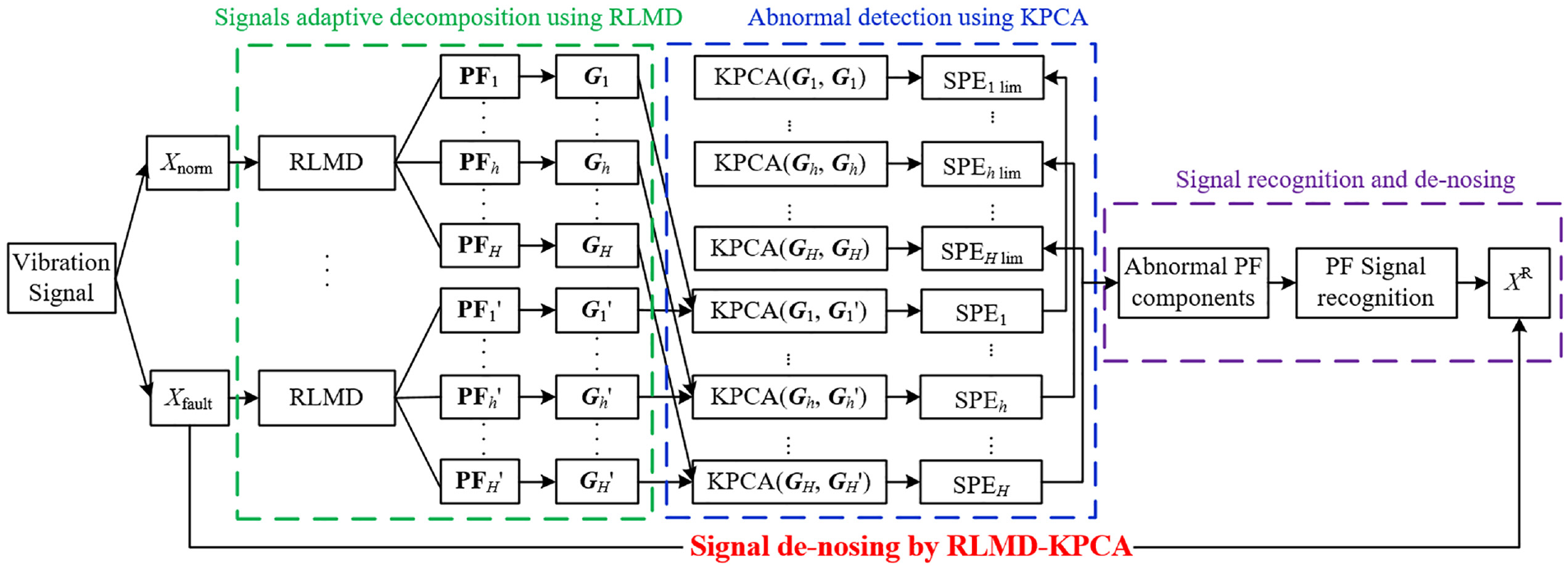
The procedure of the proposed de-noising method.

Numerical verification and experimental analysis

Numerical verification

To validate the effectiveness of proposed RLMD-KPCA, a simulation test is implemented for the comparison. Several studies have utilized a series of periodic exponential decaying high-frequency oscillations to simulate the impact signal resulting from local faults in bearings (Brie, 2000). Given the structural similarity with a normal bearing, the impact oscillation signal described above is analyzed to perform signal de-noising, denoted as follows

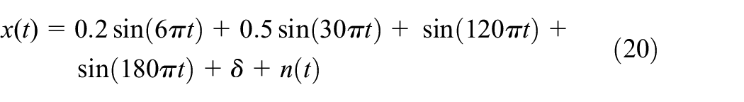
\begin{matrix} x (t) = 0.2 \sin (6 π t) + 0.5 \sin (30 π t) + \sin (120 π t) + \\ \sin (180 π t) + δ + n (t) \end{matrix}

(20)

where n(t) is the background noise. δ represents the impact oscillation signal generated by bearing local fault, which is defined by

δ = 10 \cdot \sin (200 t) \cdot \exp (- 12 t)

(21)

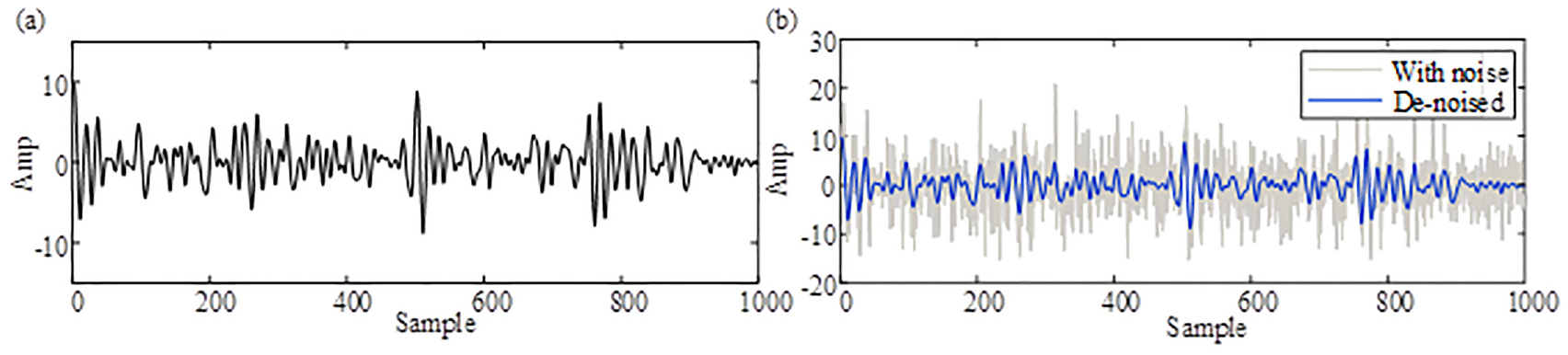
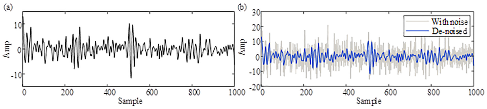
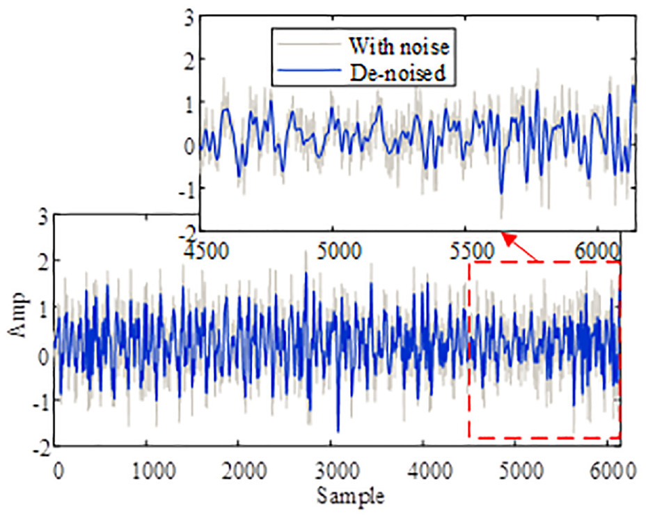
Vibration data is generated by 4 times impact oscillation with a sampling rate of 1 kHz for 1000 sampling points. Figure 2 depicts the normal and fault signals with and without noise. It is evident from Figure 2(b) and (d) that both the normal and fault signals are almost completely obscured by noise.

Figure 2.

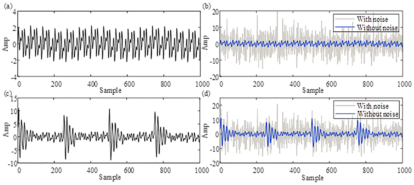
Simulated signals: (a) normal signal without noise, (b) normal signal with noise, (c) fault signal without noise, and (d) fault signal with noise.

Abnormal recognition using KPCA-SPE

To evaluate the abnormal recognition ability of KPCA-SPE, the simulated fault vibration signals are employed for the test. Normal operation signals of bearing are utilized to establish the baseline model, while fault signals are used for abnormal recognition. To demonstrate the effectiveness of KPCA-SPE, the other three models, namely, PCA-SPE, PCA-T², and KPCA-T², are calculated to carry out the comparison.

After the establishment of the baseline model, the results obtained by different methods are presented in Figure 3. The first 250 data points in Figure 3 represent the statistics calculated using a normal signal, and the last 250 data points correspond to the statistics computed using a fault signal. The red dashed-dotted line defines the T²/SPE statistics threshold. It can be observed that there is no noticeable difference at the normal period, while all statistics have distinct mutation during the fault condition. Among four abnormal recognition models, SPE can reflect the abnormal vibration signal more clearly than T². The main reason is that when there is a small anomaly in the signal, its projection in the principal component space does not change significantly. Conversely, the projection in the residual space itself is very small, and even slight fluctuations caused by a small anomaly can be clearly reflected by SPE. Moreover, in both SPE and T², KPCA can detect abnormal vibration signals more accurately than PCA when bearing failure occurs. This is because the kernel function in KPCA can capture high-order nonlinear statistical information that is often ignored by PCA. Although PCA-SPE has more samples exceeding the SPE threshold in fault conditions than KPCA-SPE, it also has more samples exceeding the SPE threshold in normal conditions, which may lead to misrecognition. Consequently, the KPCA-SPE model shows a more precise abnormal recognition result compared with the other three models.

Figure 3.

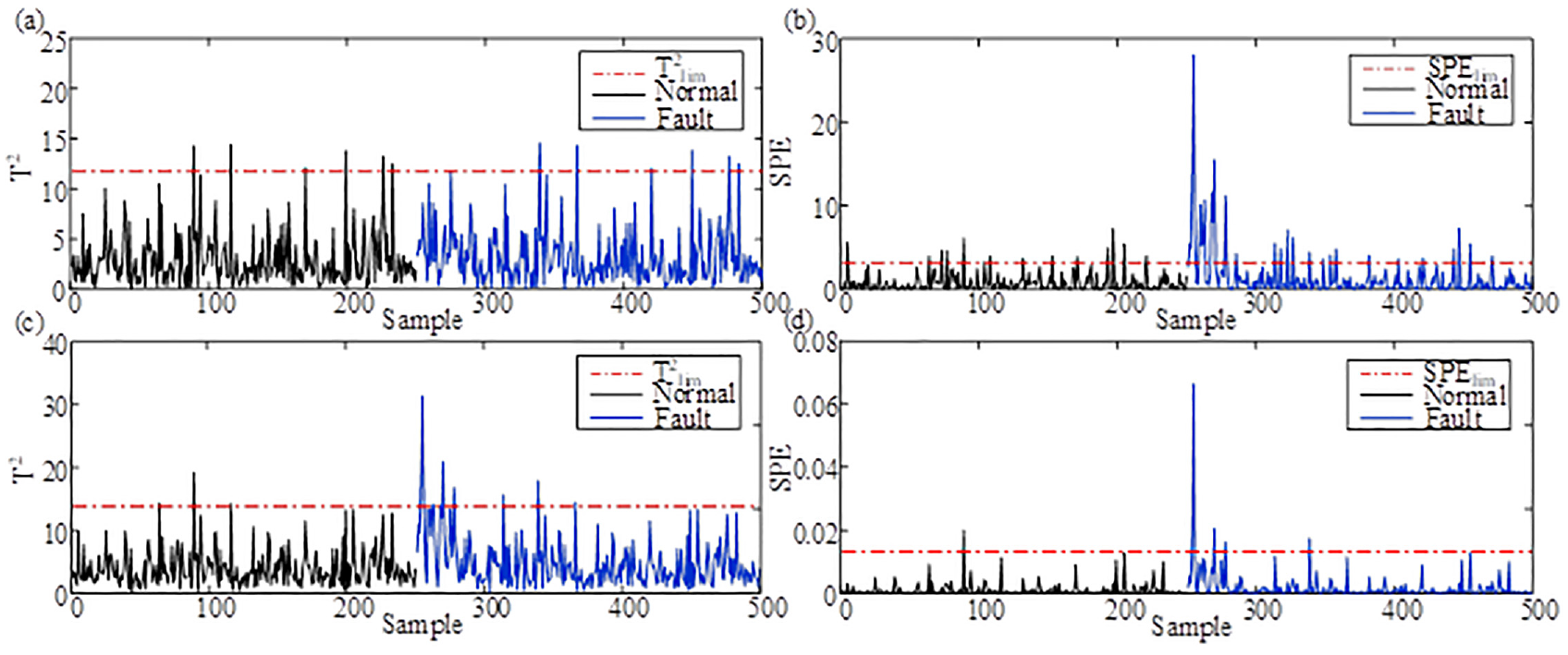
Abnormality detection comparison: (a) PCA-T², (b) PCA-SPE, (c) KPCA-T², and (d) KPCA-SPE.

Signal de-noising based on RLMD-KPCA

To demonstrate the effectiveness of RLMD-KPCA in signal de-noising, RLMD is employed to decompose normal signals and establish a baseline model using KPCA. Then the same KPCA model is used to recognize abnormal decomposed functions in fault signals. For simplicity, only a fault signal is utilized to evaluate the decomposition performance of RLMD. The results of RLMD methods on fault signal are shown in Figure 4, which reveals a series of PFs arranged in order of decreasing frequency. The high-frequency noise is mainly concentrated in the PF₁ component, while the four impact components are included in the PF₂ component. After signal decomposition, fault component recognition can be performed.

Figure 4.

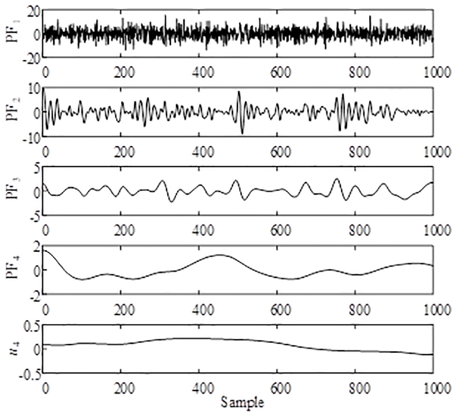
Signal decomposition of RLMD.

After implementing the abnormal recognition, Figure 5 illustrates the KPCA-SPE for the fault PFs. From Figure 5, we can find that SPE of PF₂ and u₄ exceeds the threshold value obviously, indicating the presence of fault-related components in these PFs. By means of the decomposition and reconstruction through the RLMD-KPCA method, Figure 6 shows the de-noised fault signal. The results indicate that RLMD-KPCA can remove the majority of the noise, thereby revealing clearer fault features that were previously obscured. In particular, impact components are mined more obviously through RLMD-KPCA from the details.

Figure 5.

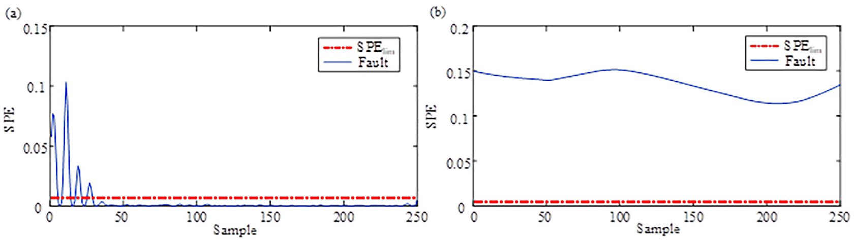
RLMD-KPCA abnormal PF detection: (a) PF₂ and (b) u₄.

Figure 6.

Signal de-noising of RLMD-KPCA: (a) de-noised signal without noise and (b) de-noised signal with noise.

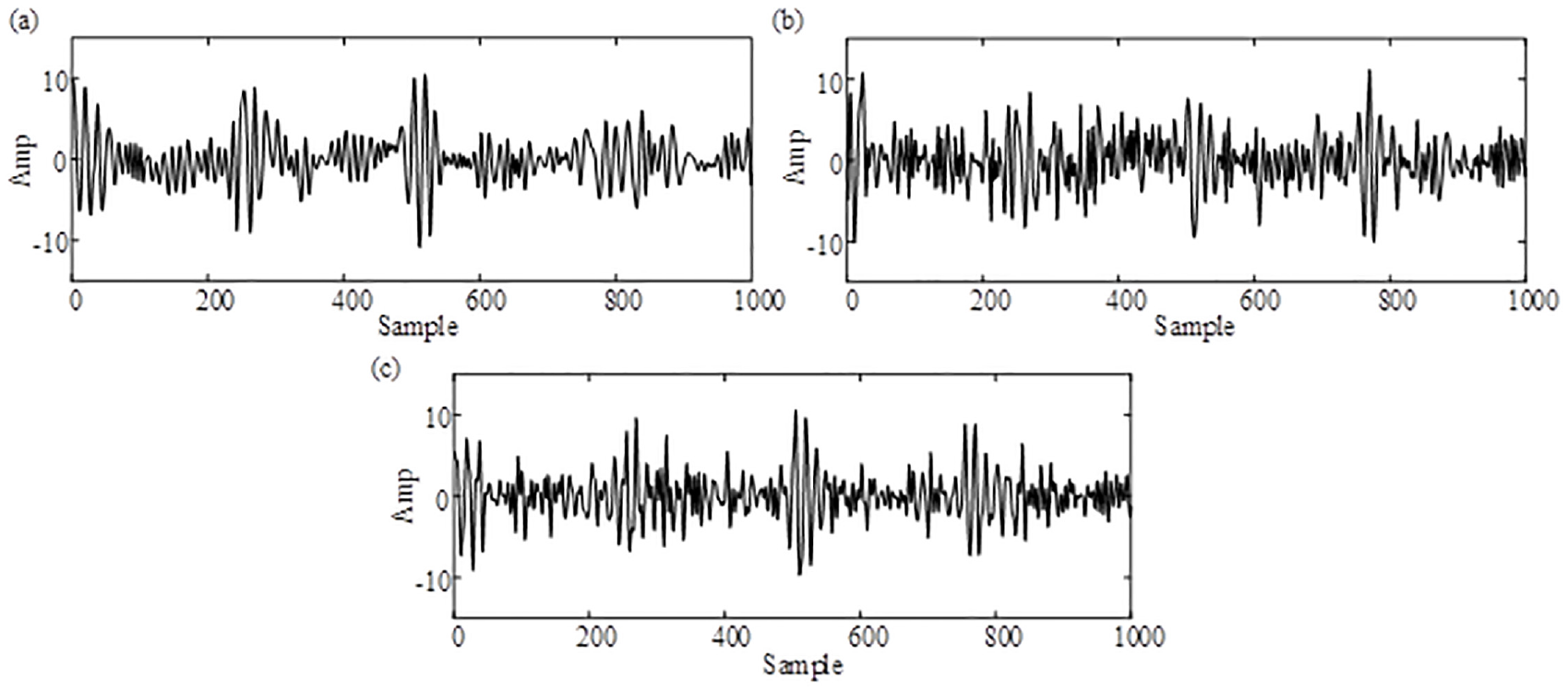
To verify the effectiveness of the proposed signal decomposition, EMD-KPCA, EEMD-KPCA, LMD-KPCA, and variational mode decomposition (VMD)-KPCA are tested on the simulated signal. For the ease of understanding, only EEMD is used to reveal the decomposition performance. After the decomposition of the fault signal, the results obtained by EEMD are shown in Figure 7. A series of IMFs with frequencies from high to low can be obtained through EEMD. However, the functions decomposed by the EEMD method are more than RLMD, and the high-frequency noise is concentrated in the component PF₁. Moreover, most of the functions decomposed by EEMD contain multiple noise components, and the number of functions is large, which increases the computational complexity of the algorithm. Therefore, RLMD demonstrates a high level of decomposition efficiency, as evidenced by the comparison of decomposition results. Furthermore, after implementing abnormal recognition, Figure 8 depicts the KPCA-SPE for fault PFs. It can be observed that the SPE of IMF₃, IMF₄, IMF₆, IMF₈, and u₈ exceeds the threshold value obviously, indicating the presence of fault components in the associated PFs. Figure 9 demonstrates the de-noised fault signal through decomposition and reconstruction using the EEMD-KPCA method. The results indicate that EEMD-KPCA is capable of removing a significant amount of noise. However, the impact components show some level of noise interference compared with the RLMD-KPCA method. Consequently, it is evident that RLMD-KPCA provides better signal de-noising performance than EEMD-KPCA.

Figure 7.

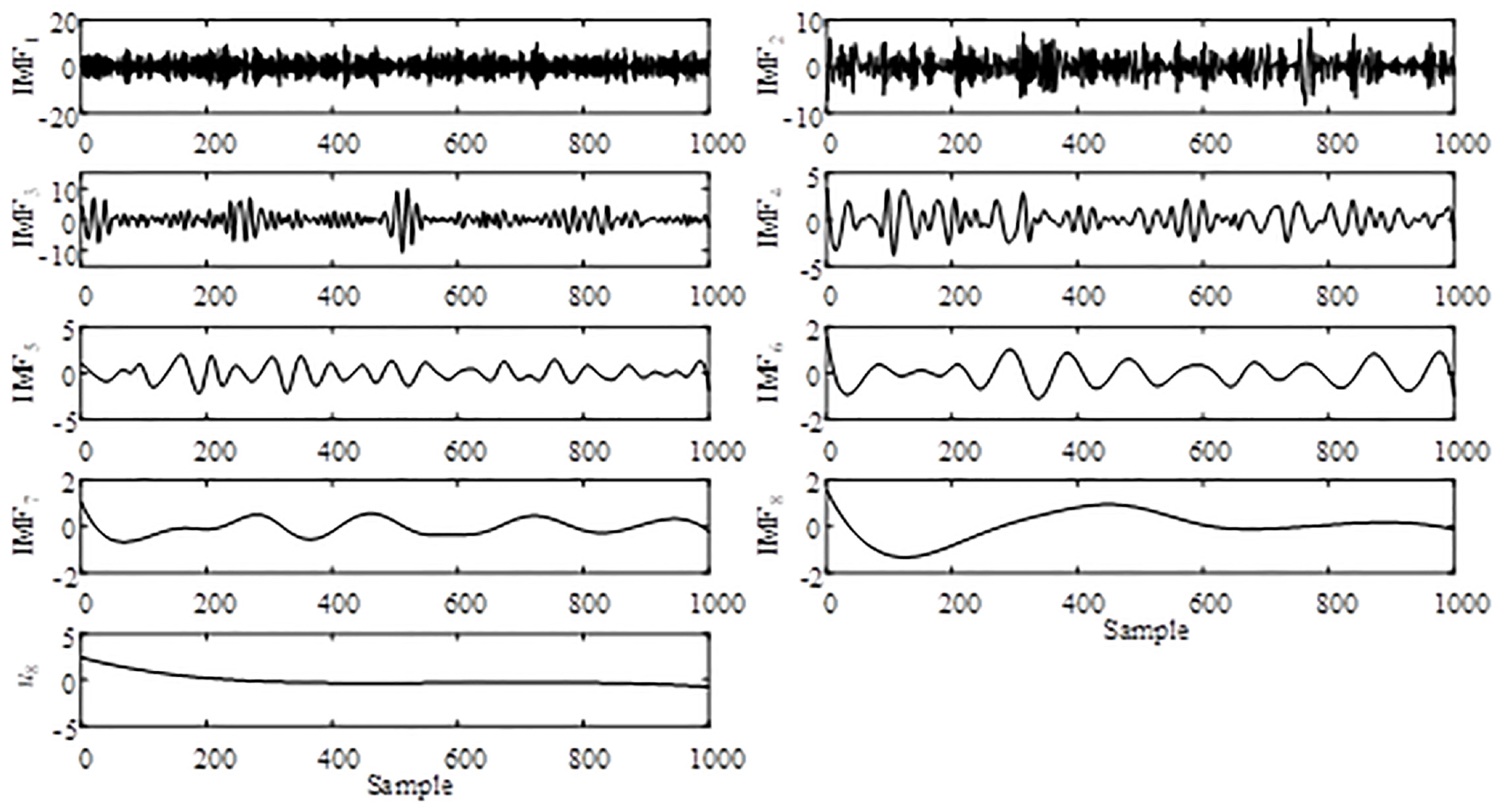
Signal decomposition of EEMD.

Figure 8.

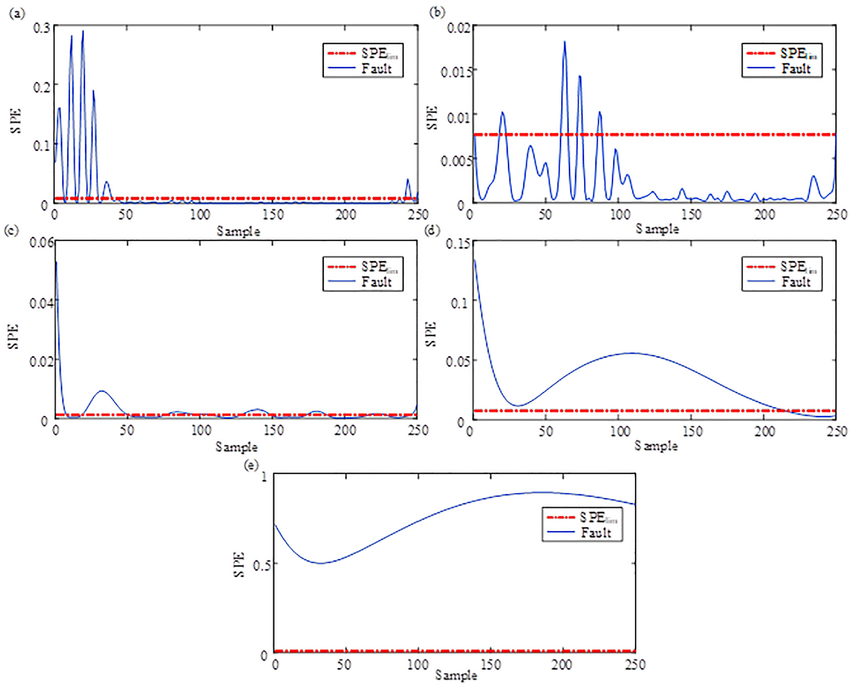
EEMD-KPCA abnormal IMF detection: (a) IMF₃, (b) IMF₄, (c) IMF₆, (d) IMF₈, and (e) u₈.

Figure 9.

Signal de-noising of EEMD-KPCA: (a) de-noised signal without noise and (b) de-noised signal with noise.

In addition, we carried out comparisons with EMD-KPCA, LMD-KPCA, and VMD-KPCA methods. The de-noising steps are the same as EEMD-KPCA and RLMD-KPCA, but the only difference is that they use different signal decomposition methods. Figure 10 depicts the de-noised results of EMD-KPCA, LMD-KPCA, and VMD-KPCA. Intuitive observation of Figure 10 reveals that all three de-noised signals suffer from noise interference compared with EEMD-KPCA and RLMD-KPCA. The main reason to explain this phenomenon is the mode mixing problem in EMD, LMD, and VMD, which negatively affects the signal decomposition process.

Figure 10.

De-noised comparison: (a) de-noised signal by EMD-KPCA, (b) de-noised signal by LMD-KPCA, and (c) de-noised signal by VMD-KPCA.

To further investigate the performance of kernel function mapping in the abnormal recognition model of KPCA, PCA is selected as the fault selection model. The recognition results are presented in Figure 11, which is consistent with the results obtained using KPCA (Figure 5), with PF₂ and u₄ recognized as fault components. However, as observed in Figure 3, PF₄ is misrecognized as a fault component in comparison with KPCA. After the reconstruction with PF₂, PF₄, and u₄, Figure 12 shows the de-noised comparison between RLMD-PCA and RLMD-KPCA. Owing to the addition of the PF₄ component, the amplitude of RLMD-PCA is higher than that of RLMD-KPCA. Nonetheless, there is no apparent difference between the two de-noised signals. However, we will carry out a detailed comparison as presented in Table 2.

Figure 11.

RLMD-PCA abnormal PF detection: (a) PF₂, (b) PF₄, and (c) u₄.

Figure 12.

De-noised comparison: (a) de-noised signal by RLMD-PCA and (b) de-noised signal by RLMD-KPCA.

The comparison of fault selection strategies using different decomposition methods reveals that RLMD-KPCA can effectively improve decomposition accuracy and save computation time. However, the analysis mainly focuses on the fault selection strategy based on multiscale analysis. Another issue related to fault selection is how different traditional selection strategies affect fault selection accuracy. For the purposes of comparison, we selected three additional strategies to evaluate the effectiveness of the proposed KPCA fault selection strategy: (a) correlation coefficient criterion (Ma et al., 2018), (b) kurtosis criterion (Zhao et al., 2021), and (c) the combination of above two. To conduct a fair comparison, RLMD is utilized as the same decomposition method. Therefore, three different methods were applied to the signal de-noising of slewing bearing using the same vibration data.

Table 1 lists the detailed evaluating parameters of decomposed components. It is found that PF₁∼PF₂ of RLMD-correlation coefficient criterion are determined as fault-related PFs, which are greater than 0.25. On the contrary, PF₂ of RLMD-kurtosis criterion is determined as fault-related PFs, which is greater than 3. Combining these two criteria, PF₂ of RLMD-correlation coefficient criterion + kurtosis criterion is determined as fault-related PFs. Figure 13 shows the comparison of de-noised fault signals through these three methods. It can be observed that kurtosis criterion-related methods (Figure 13(b) and (c)) have similar signal de-noising effects to RLMD-KPCA. However, the RLMD-correlation coefficient criterion shows the worst de-noising effect owing to the misrecognition of noise component PF₁. Intuitively, there is no significant difference between RLMD-kurtosis criterion and RLMD-correlation coefficient criterion + kurtosis criterion when compared with RLMD-KPCA, and the superiority of RLMD-KPCA will be verified below. Furthermore, all three methods are sensitive to abnormal recognition of medium-frequency components but less sensitive to low-frequency components. Conversely, RLMD-KPCA has the ability to recognize both medium-frequency and low-frequency fault components, highlighting the superiority of weak low-frequency signal de-noising.

Table 1.

Parameters of decomposed components.

Parameter	PF₁	PF₂	PF₃	PF₄	u ₄
Correlation coefficient	0.8650	0.5429	0.1864	0.0820	0.0215
Kurtosis index	2.9814	4.6069	2.8142	2.5444	1.8309

PF: product function. Bold font of Correlation coefficient means value is greater than 0.25. Bold font of Kurtosis index means value is greater than 3.

Figure 13.

De-noised comparison: (a) de-noised signal by RLMD-correlation coefficient criterion, (b) de-noised signal of RLMD-kurtosis criterion, (c) de-noised signal by RLMD-correlation coefficient criterion + kurtosis criterion, and (d) de-noised signal of RLMD-KPCA.

To quantitatively evaluate the performance of each method in signal de-noising, the mean squared error (MSE) and the signal-noise ratio (SNR) are calculated to carry out the comparison. The mathematical expressions of MSE and SNR are as follows

MSE = \frac{1}{m} \sum_{i = 1}^{m} {(x_{i} - {\hat{x}}_{i})}^{2}

(22)

SNR = 10 \log_{10} (\frac{\sum {x_{i}}^{2}}{\sum {(x_{i} - {\hat{x}}_{i})}^{2}})

(23)

where $x_{i}$ is the signal without noise, ${\hat{x}}_{i}$ represents the de-noised signal, and m denotes the number of samples.

In addition, the computational cost of each method is compared in terms of signal decomposition time. Table 2 presents the MSE, SNR, and decomposition time t of the de-noised signal obtained from EMD-KPCA, EEMD-KPCA, LMD-KPCA, VMD-KPCA, RLMD-PCA, and RLMD-KPCA. The evaluation indicators of three traditional de-noising methods are listed in Table 3. EEMD-KPCA performs better than EMD-KPCA in terms of de-noising effect due to the elimination of mode mixing. However, its decomposition efficiency is inferior to that of EMD-KPCA. Furthermore, the decomposition speed of LMD-related methods is much faster than EMD-related methods owing to the decrease in iteration number. However, the de-noising effect of LMD-KPCA is worse than that of EMD-related methods in terms of MSE and SNR. Evaluating indicators of VMD-KPCA are worse than those of RLMD-KPCA. Hence, RLMD-KPCA has the merit of more accurate signal de-noising than RLMD-PCA, highlighting the superiority of kernel function mapping for abnormal recognition. Meanwhile, similar to Figure 13, RLMD-correlation coefficient criterion performs worse than other methods in signal de-noising. Although RLMD-kurtosis criterion and RLMD-correlation coefficient criterion + kurtosis criterion get better de-noised effect than EMD-KPCA, EEMD-KPCA, LMD-KPCA, RLMD-PCA, and RLMD-correlation coefficient criterion, their evaluating indicators are inferior to RLMD-KPCA. Among these nine methods, the MSE and decomposition time t of RLMD-KPCA are slightly lower, while the SNR is higher. This indicates that the proposed method can significantly enhance the decomposition efficiency, suppress noise, and bring the de-noised signal closer to the row fault vibration signal. Therefore, the RLMD-KPCA method shows better results with respect to the other eight methods.

Table 2.

Evaluating indicators of de-noised signals.

Parameter	MSE	SNR	t (seconds)
EMD-KPCA	5.2869	0.3842	0.026
EEMD-KPCA	4.8596	0.7502	4.983
LMD-KPCA	6.3804	−0.4323	0.005
VMD-KPCA	3.9370	1.6646	0.634
RLMD-PCA	3.9433	1.6576	0.106
RLMD-KPCA	3.7129	1.9190	0.106

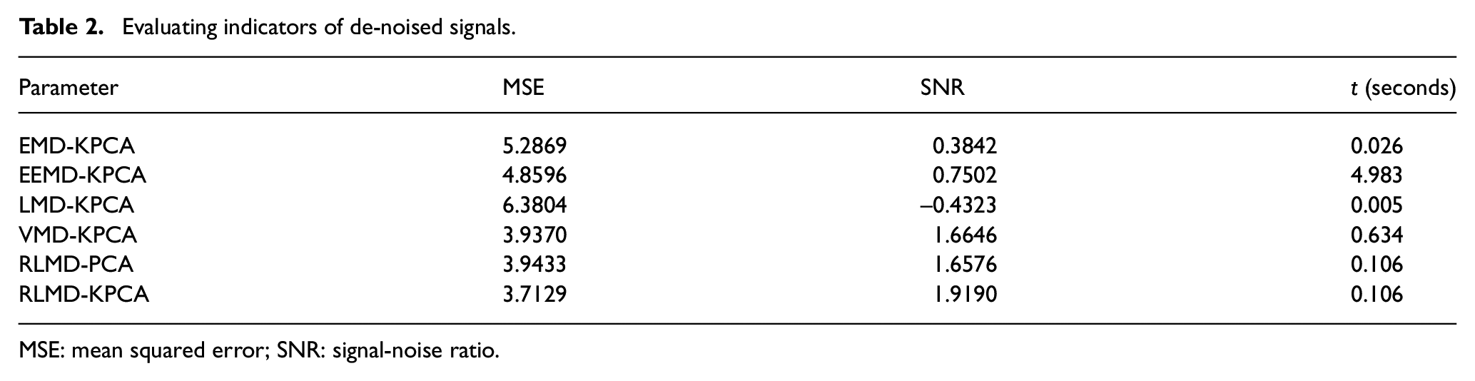
MSE: mean squared error; SNR: signal-noise ratio.

Table 3.

Evaluating indicators of de-noised signals based on traditional methods.

Parameter	MSE	SNR	t (seconds)
RLMD-correlation coefficient criterion	24.0530	−6.1955	0.106
RLMD-kurtosis criterion	3.7317	1.8971	0.106
RLMD-correlation coefficient criterion + kurtosis criterion	3.7317	1.8971	0.106
RLMD-KPCA	3.7129	1.9190	0.106

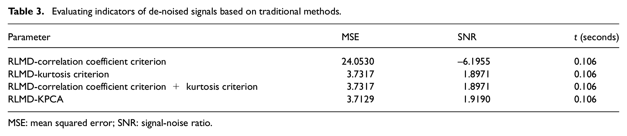
MSE: mean squared error; SNR: signal-noise ratio.

Experimental analysis

Slewing bearing test rig

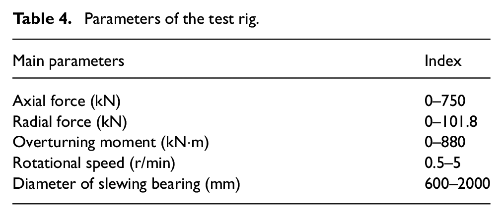
A large-size low-speed slewing bearing test rig is designed to simulate actual working conditions, as illustrated in Figure 14(a). The test rig is composed of the following main components: (a) Mechanical structure. The top and bottom flame are connected with the main and accompanied slewing bearing to transfer load, with installing brackets supporting the radial force. (b) Slewing bearing. Main slewing bearing links with accompanied test slewing bearing through the bolt, constituting back-to-back structure. (c) Hydraulic system. The linkage of hydraulic cylinder G1 and G2 generates the axial force and overturning moment, while hydraulic cylinder G3 provides radial force. The pinion is turned by hydraulic motor G4, driving slewing bearing to rotate through gear meshing. (d) Measuring-control system. SIMENS S7-200 connects with hydraulic cylinders and hydraulic motor to realize the loading control. Upper computer communicates with SIMENS S7-200 through object linking and embedding (OLE) for Process Control (OPC) protocol. Vibration, temperature (Figure 14(b)), and torque (Figure 14(c)) signals generated from slewing bearing are acquired by NI cDAQ module. The main parameters of the test rig are listed in Table 4.

Figure 14.

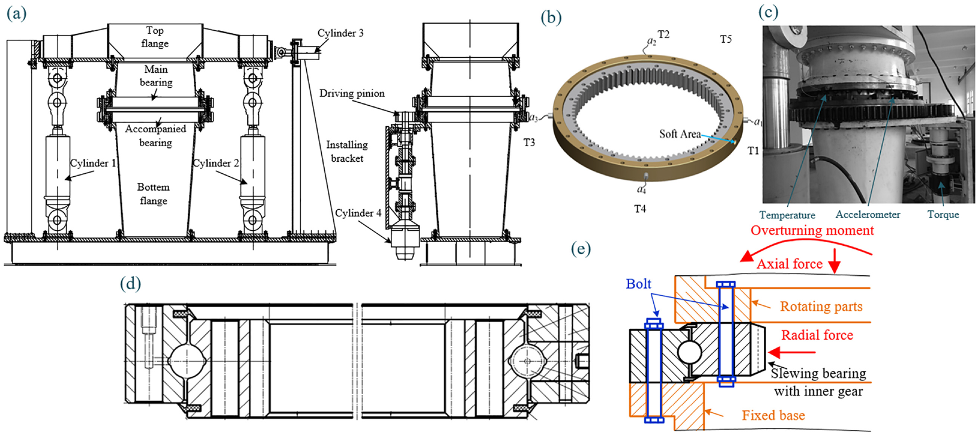
Experimental description: (a) test rig, (b) the distribution of the sensors over the fixed ring raceway. (c) HALT, (d) test bearing (single-row four-point contact ball slewing bearing), and (e) diagram of applied loads.

Table 4.

Parameters of the test rig.

Main parameters	Index
Axial force (kN)	0–750
Radial force (kN)	0–101.8
Overturning moment (kN·m)	0–880
Rotational speed (r/min)	0.5–5
Diameter of slewing bearing (mm)	600–2000

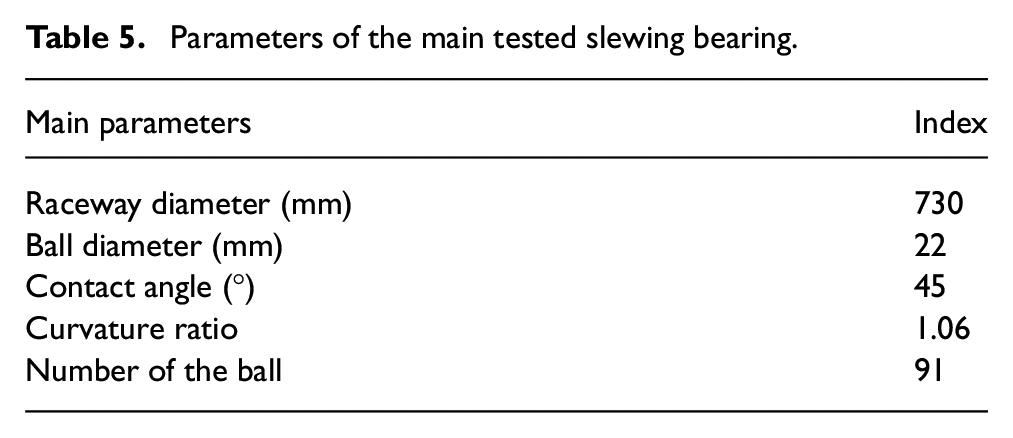
The test slewing bearing used in the accelerated life test is a single-row four-point contact ball structure with an inner gear (Figure 14(d)). It consists of an inner ring, outer ring, ball, and cage. Unlike small-size high-speed bearing, the inner and outer rings of slewing bearing (Figure 14(b)) have several bolt holes that are distributed to link the upper and lower structural components. The inner ring has gear teeth that drive parts to rotate, such as wind turbine blade and tunnel boring machine cutter head. Conversely, the outer ring is fixed with the base structure. Table 5 shows the detailed properties of the test slewing bearing. It is worth noting that shortening the test time without changing the fatigue capacity of bearing is a challenge to all manufacturers. To accelerate the test, the slewing bearing is subjected to a limited combination of extreme force (Figure 14(e)). Hence, the test speed is suggested as a rated working speed of 4 r/min.

Table 5.

Parameters of the main tested slewing bearing.

Main parameters	Index
Raceway diameter (mm)	730
Ball diameter (mm)	22
Contact angle (°)	45
Curvature ratio	1.06
Number of the ball	91

The load distribution along the circumference of slewing bearing is subjected to a combination of axial force, radial force, and overturning moment resulting in two heavy-load regions and two light-load regions. Therefore, four accelerometer sensors are mounted at every 90 degree measuring interval (Figure 14(b)). Besides, four RTD sensors are inserted into lubricating grease filling holes to measure the lubricating oil temperature of the raceway (Figure 14(b)), and an resistance temperature detector (RTD) sensor (T5) is utilized to measure atmospheric temperature and eliminate interference. A torque sensor located at the connection between the hydraulic motor and pinion (Figure 14(c)) indirectly monitors the friction torque and rotational speed of slewing bearing. Considering different signal characteristics, the sample rate of the vibration signal is set at 2048 Hz, and the rest is set at 10 Hz.

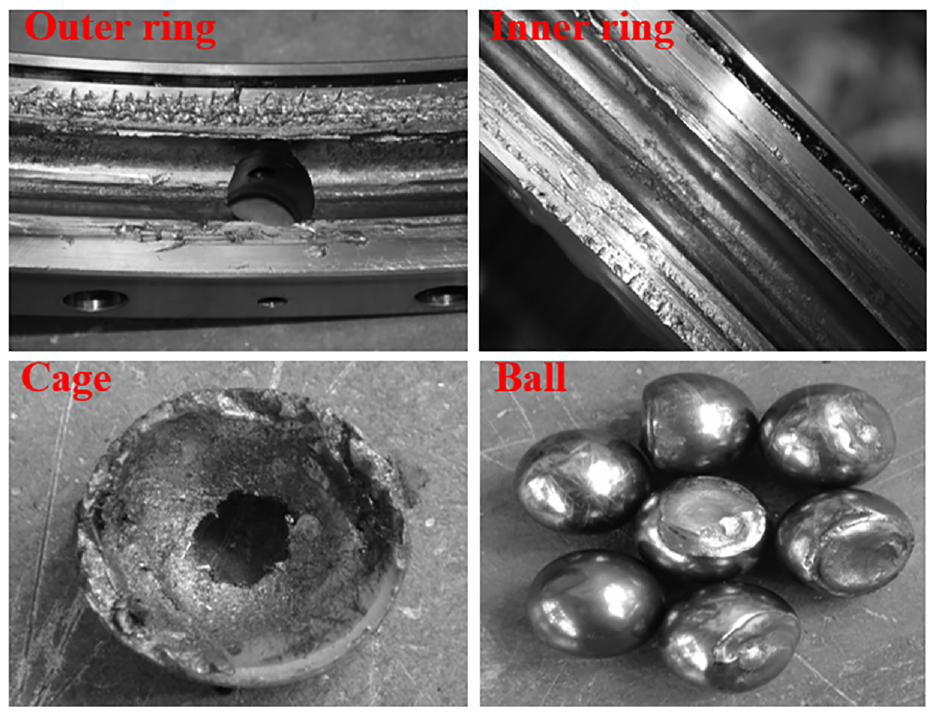
After the accelerated life test, the slewing bearing got stuck and a failure happened. It is well known that the status of the slewing bearing should be established according to the relationship with monitored signals. However, the dismantlement of the whole test rig to inspect the health status of the slewing bearing is unacceptable in light of manpower and cost. The health condition of the bearing raceway, ball, and cage at the end of the test is shown in Figure 15. The spalling, pitting, and stretch damage happened not only to the raceway but also to the ball and cage.

Figure 15.

Damage components of slewing bearing.

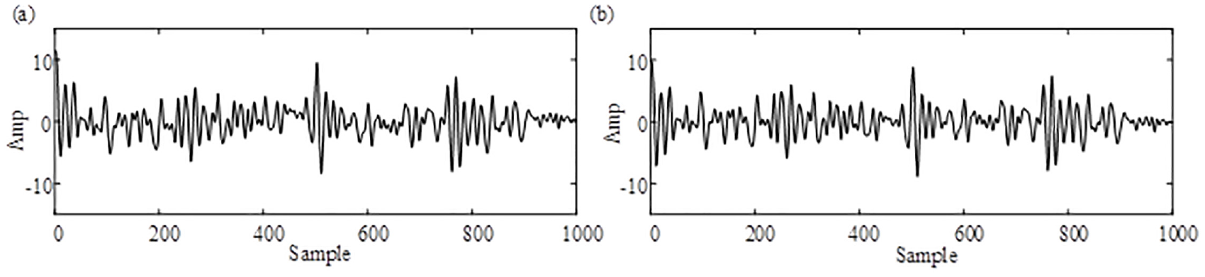
Figure 16 displays the vibration signals obtained from two different periods: normal and fault signals. From raw vibration signals, we can observe a noticeable increase in the amplitude of vibration signals as the fault deteriorates. The vibration component predominantly comprises high-frequency noise, while periodic fault impacts gradually emerge with the occurrence of faults. However, due to the presence of strong background noise in the original vibration signals, it becomes challenging to extract relevant fault information from the vibration signal.

Figure 16.

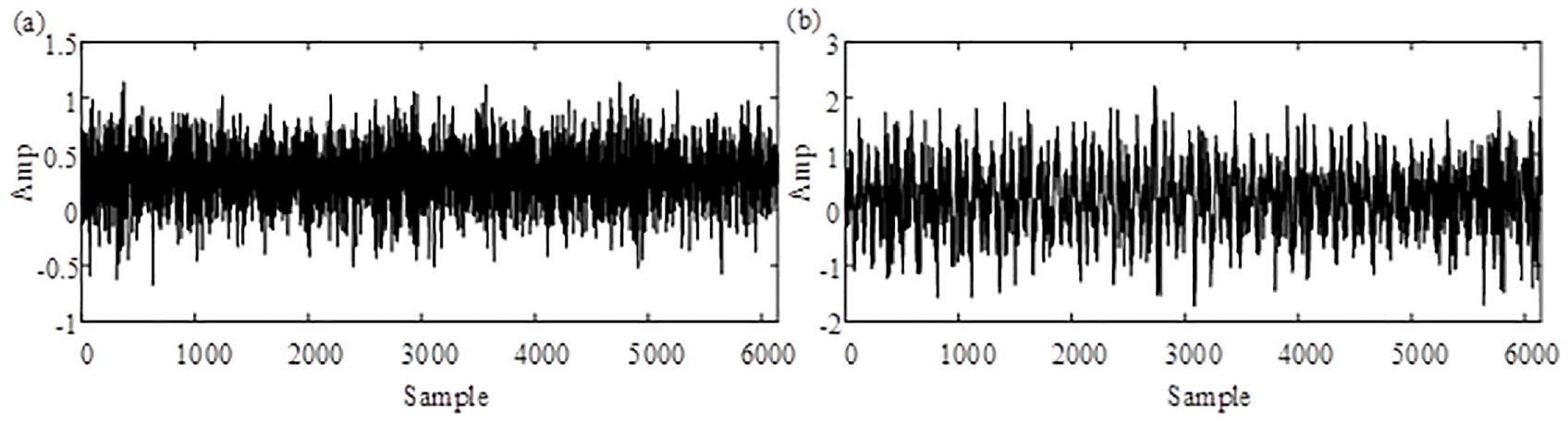
Raw vibration signals of slewing-bearing life test: (a) normal signal and (b) outer ring fault signal.

Data processing

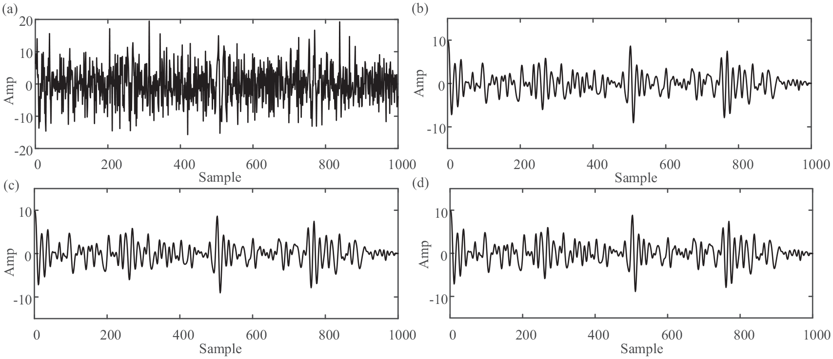
The proposed RLMD-KPCA is applied to signal de-noising according to the procedure shown in Figure 1. First, implement RLMD on normal and fault signals to obtain PFs. Second, split PF into the multi-dimensional matrix, with the normal matrix serving as the healthy KPCA model, and map the multi-dimensional matrix into the healthy KPCA model getting the SPE statistics. Third, select the PFs of each segment which exceed the SPE threshold. Finally, obtain the reconstructed signal. For the sake of simplicity, the outer ring fault vibration signal is taken as an example for signal decomposition, as shown in Figure 17. Following the decomposition of RLMD, a series of PFs with decreasing frequency can be obtained. High-frequency noise is concentrated in the component PF₁, while the periodic components are included in the component PF₂∼u₄. After signal decomposition, fault selection can be carried out.

Figure 17.

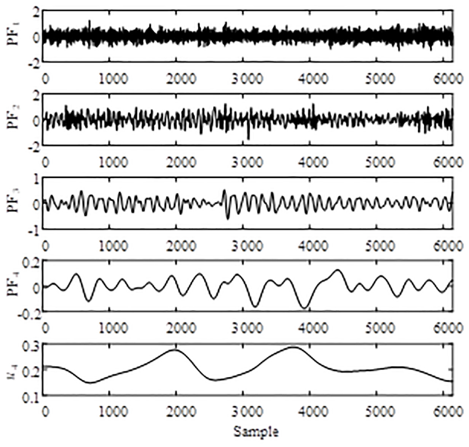
Outer ring fault signal decomposition of RLMD.

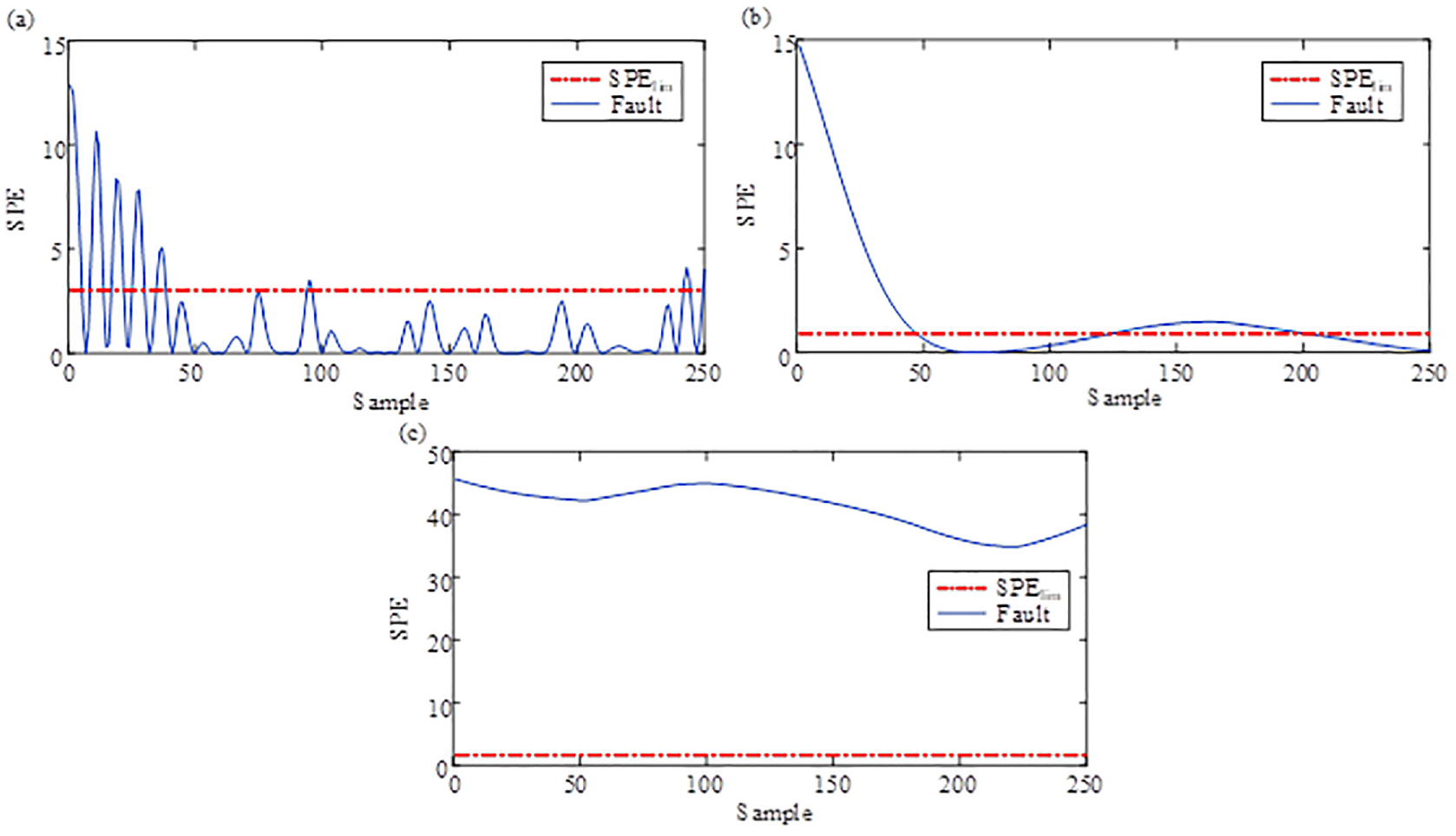
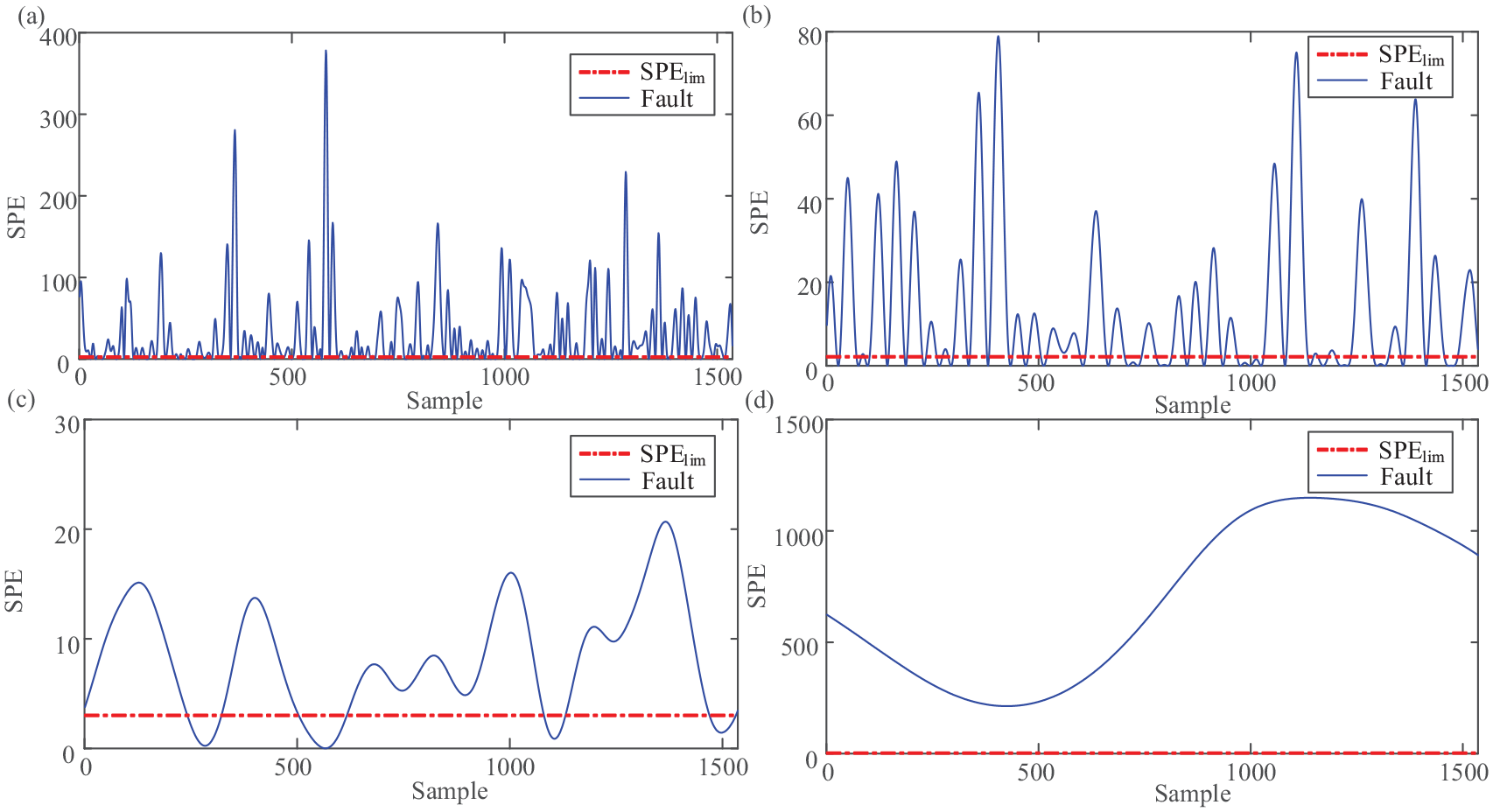
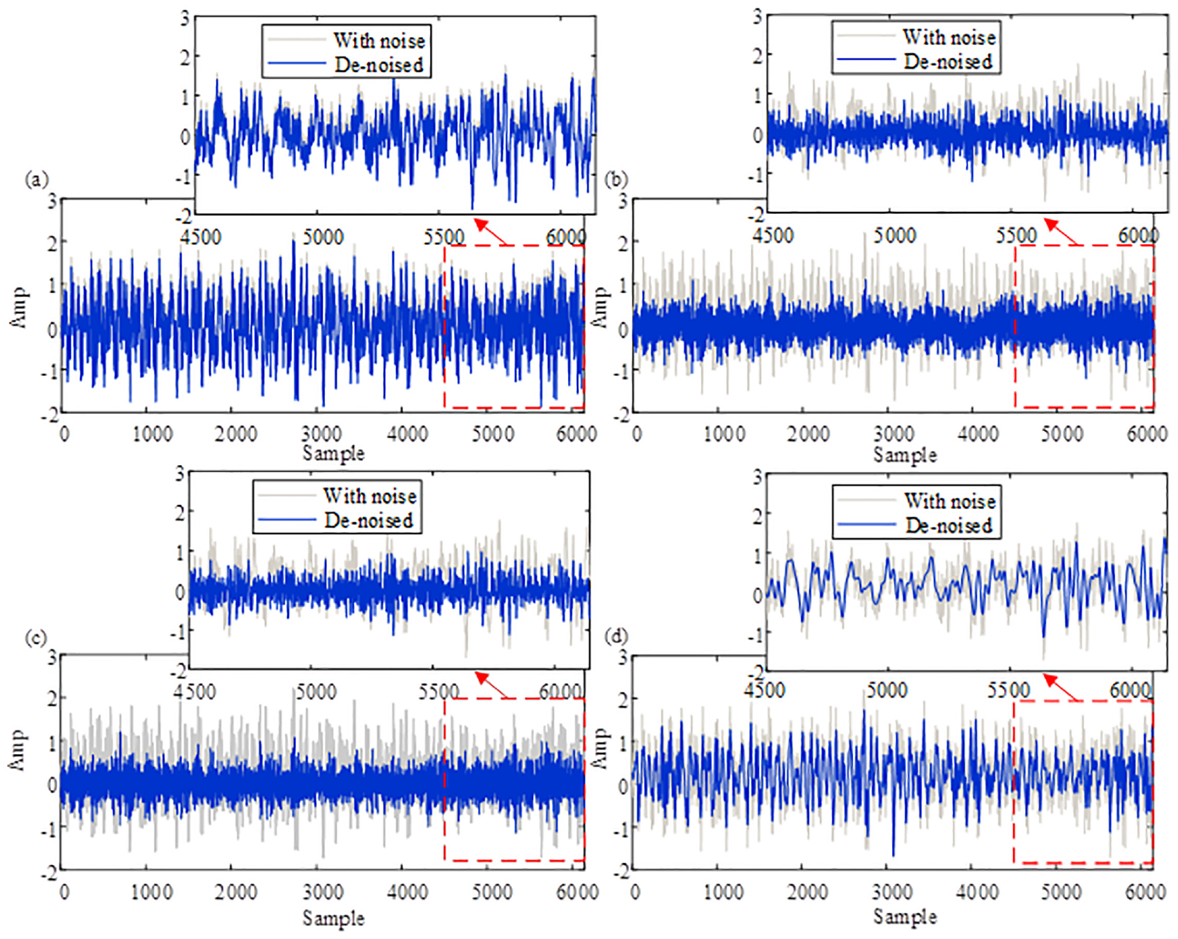
Following the implementation of abnormal recognition, Figure 18 illustrates the KPCA-SPE result for the fault PFs. As shown in Figure 18, the SPE of the PF₂, PF₃, PF₄, and u₄ exceeds the threshold value obviously, indicating that these related PFs contain fault components. These PFs are then selected to reconstruct the signal. Figure 19 displays the original and reconstructed signals using the RLMD-KPCA. To facilitate comparison, EMD-KPCA, EEMD-KPCA, LMD-KPCA, and VMD-KPCA are utilized to verify the advantage of the RLMD-KPCA, as shown in Figure 20. For a detailed comparison, the purple dotted rectangular region in Figures 19 and 20 is enlarged. From Figures 19 and 20, we can intuitively observe that VMD-KPCA shows the worst performance than other methods, and there exists noise interference in EMD-KPCA and LMD-KPCA de-noised signals compared with EEMD-KPCA and RLMD-KPCA. The main reason to explain this phenomenon is the mode mixing problem associated with EMD and LMD, which affects the signal decomposition effect. Hence, it is obvious that the proposed RLMD-KPCA method clearly highlights the fault periodic impulse information in comparison with EEMD-KPCA. Through the comparison of different decomposition methods, RLMD has a merit of high decomposition accuracy.

Figure 18.

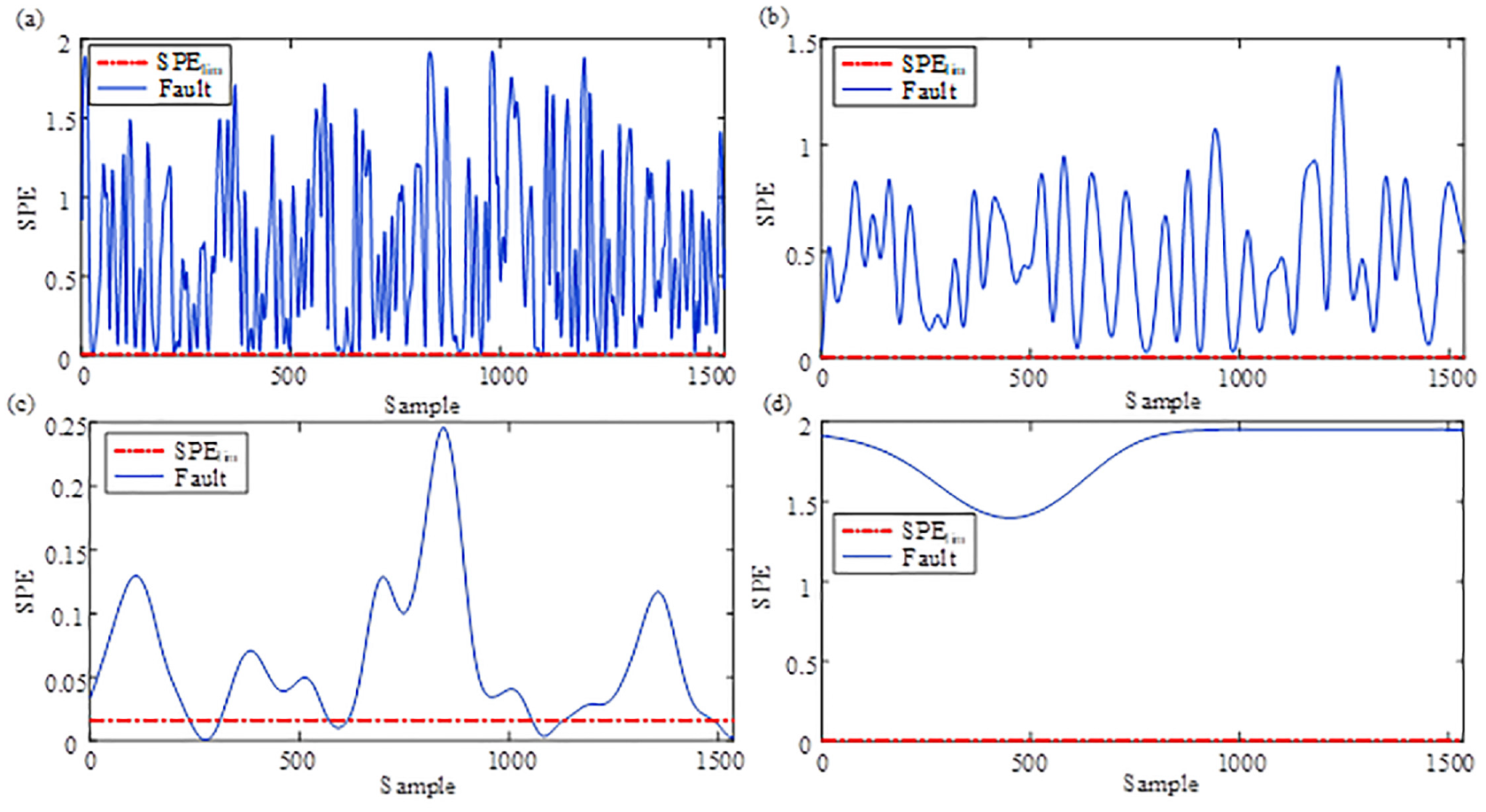
RLMD-KPCA abnormal PF detection: (a) PF₂, (b) PF₃, (c) PF₄, and (d) u₄.

Figure 19.

De-noised signal of RLMD-KPCA.

Figure 20.

De-noised comparison: (a) de-noised signal by EMD-KPCA, (b) de-noised signal of EEMD-KPCA, (c) de-noised signal by LMD-KPCA, and (d) de-noised signal of VMD-KPCA.

Moreover, we implement RLMD-PCA to confirm the effectiveness of kernel function mapping. The abnormal PF detection results are depicted in Figure 21, which shows that PF₂, PF₃, PF₄, and u₄ are recognized as fault components, similar to RLMD-KPCA. Consequently, the de-noised effect of RLMD-PCA is identical to that of RLMD-KPCA. Besides, it should be noted that the difference between normal and fault signals of slewing bearing is more noticeable than that of simulated bearing signal, indicating that abnormal recognition can be easily realized through multiscale analysis such as PCA and KPCA. However, such an obvious abnormal recognition is not apparent in the simulation signal (Figures 5 and 11) owing to the little difference between normal and fault signals. The reason to explain this phenomenon is that PCA has poor ability to capture weak signal differences, whereas KPCA is suitable for weak signal abnormal recognition with the aid of kernel function mapping.

Figure 21.

RLMD-PCA abnormal PF detection: (a) PF2; (b) PF3; (c) PF4; (d) u₄

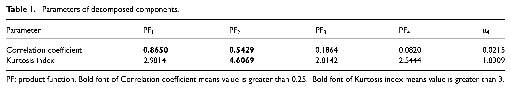
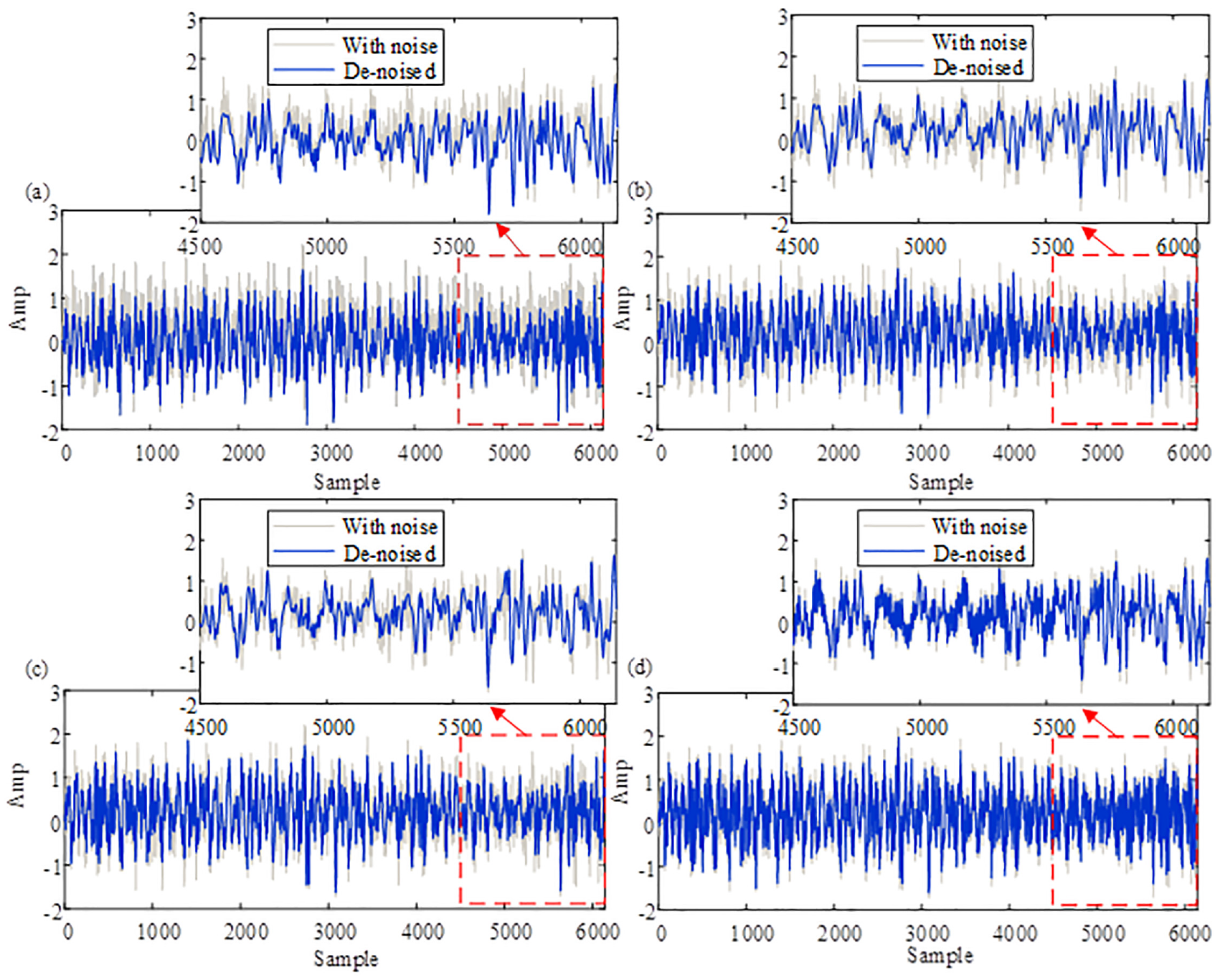
To further validate the effectiveness of RLMD-KPCA, the other three traditional signal de-noising methods are carried out for a comparison with the same fault signal. Table 6 lists the detailed evaluating parameters of decomposed components. It is found that PF₁, PF₂, and PF₃ of RLMD-correlation coefficient criterion are determined as fault-related PFs with a correlation coefficient greater than 0.25, while PF₁ and PF₄ of RLMD-kurtosis criterion are determined as fault-related PFs with a kurtosis index greater than 3. As a result, PF₁ of RLMD-correlation coefficient criterion + kurtosis criterion is determined as fault-related PF, which satisfies both criteria. The comparison of de-noised fault signals through the decomposition and reconstruction using these three methods is shown in Figure 22. It can be seen that all three traditional methods suffer from noise interference owing to the misrecognition of noise component PF₁. Furthermore, RLMD-kurtosis criterion and RLMD-correlation coefficient criterion + kurtosis criterion are basically corrupted with strong working noise. Therefore, the results highlight the superiority of proposed method in signal de-noising for such low signal-to-noise vibration signals.

Table 6.

Evaluating indicators of de-noised fault signals.

Parameter	PF₁	PF₂	PF₃	PF₄	u ₄
Correlation coefficient	0.5856	0.8261	0.5380	0.0426	0.0043
Kurtosis index	3.2689	2.9837	2.3929	3.5486	1.1303

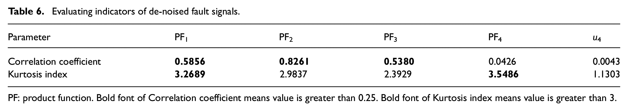
PF: product function. Bold font of Correlation coefficient means value is greater than 0.25. Bold font of Kurtosis index means value is greater than 3.

Figure 22.

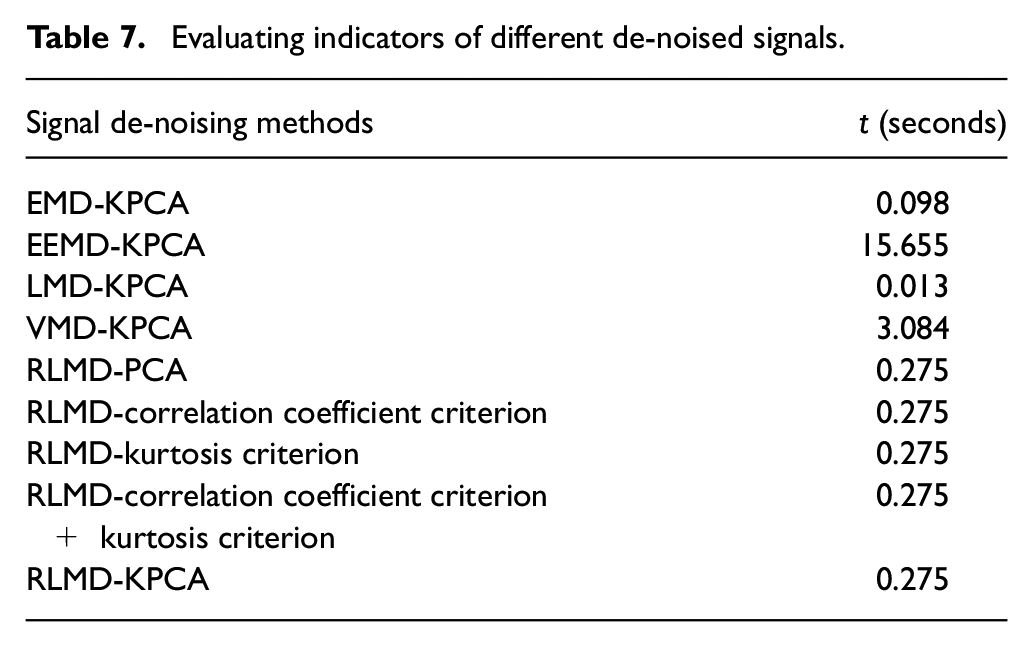
In addition, the signal decomposition time t is computed to compare the decomposition efficiency of nine methods. Considering that the fault signal without noise of slewing bearing is unavailable, MSE and SNR cannot be calculated. Table 7 lists the t of the de-noised signal based on nine methods. According to Table 7, the decomposition speed of RLMD-related methods is much faster than EEMD-related methods owing to the decrease of the iteration number. Hence, in combination with Figures 19 –22, RLMD-KPCA can effectively improve the decomposition efficiency, suppress noise, and make the de-noised signal closer to the row fault vibration signal.

Table 7.

Evaluating indicators of different de-noised signals.

Signal de-noising methods	t (seconds)
EMD-KPCA	0.098
EEMD-KPCA	15.655
LMD-KPCA	0.013
VMD-KPCA	3.084
RLMD-PCA	0.275
RLMD-correlation coefficient criterion	0.275
RLMD-kurtosis criterion	0.275
RLMD-correlation coefficient criterion + kurtosis criterion	0.275
RLMD-KPCA	0.275

To sum up, the signal-noise separation directly affects the accuracy of signal de-noising. Based on this, RLMD can improve time-frequency resolution as much as possible, which can ensure high decomposition accuracy. Under the high decomposition accuracy, statistic detection of KPCA can identify and extract those components whose signatures change significantly with the occurrence of faults. Therefore, the combination of RLMD and KPCA methods demonstrates superior performance, making it particularly well-suited for slewing bearing signal de-noising.

Conclusion and future work

This article presents a novel signal de-noising method for slewing bearing based on RLMD-KPCA. Meanwhile, statistic detection based on KPCA is employed to reconstruct fault components. The superiority of the proposed method is validated by analyzing vibration signals from a slewing-bearing life-cycle test as well as a simulated bearing fault. The signal de-noising is more visible in RLMD-KPCA, while the other combination methods (EMD-KPCA, EEMD-KPCA LMD-KPCA, VMD-KPCA, and RLMD-PCA) are inferior to it in noise reduction by means of MSE, SNR, and t. Hence, the KPCA-SPE model shows an accurate abnormal recognition result compared with the other three models (PCA-SPE, PCA-T², and KPCA-T²), and the addition of kernel function by KPCA provides an accurate fault selection model for signal de-noising than PCA. Besides, three different traditional selection strategies are selected to validate the effectiveness of the proposed KPCA fault selection strategy (correlation coefficient criterion, kurtosis criterion, and the combination of the above two strategies). The KPCA-based method can provide an accurate fault selection strategy for signal de-noising. As a result, signal de-noising based on RLMD-KPCA indicates high accuracy which makes this method more suitable for slewing bearing de-noising analysis.

The novelty of signal de-noising in this paper lies in the combination of adaptive decomposition and statistical detection. Future experiments should explore advanced adaptive decomposition methods, such as a noise-assisted approach for RLMD, and ways to improve the ability of statistical detection by employing an appropriate probability model for KPCA. In addition, experiments will mainly focus on other low-speed heavy-load large-size rotating machinery to verify the generality of this method or find the problems in generalizing it.

Footnotes

Declaration of conflicting interests

The author(s) declared no potential conflicts of interest with respect to the research, authorship, and/or publication of this article.

Funding

The author(s) disclosed receipt of the following financial support for the research, authorship, and/or publication of this article: This work was financed by the Project funded by the National Natural Science Foundation of China (grant no. 52205106), the Natural Science Foundation of Jiangsu Province (grant no. BK20210547), the Science Research of Colleges Universities in Jiangsu Province (grant no. 21KJB460036), the China Postdoctoral Science Foundation (grant no. 2021M691558), and the Jiangsu Postdoctoral Research Grants Program (grant no. 2021K297B).

ORCID iD

Yubin Pan

Data availability statement

Data sharing is not applicable to this article as no datasets were generated or analyzed during the current study.

References

Amasorrain

Sagartzazu

Damián

(2003) Load distribution in a four contact-point slewing bearing. Mechanism and Machine Theory 38(6): 479–496.

Bakshi

(1998) Multiscale PCA with application to multiscale statistical process monitoring. AIChE Journal 44(7): 1596–1610.

Brie

(2000) Modelling of the spalled rolling element bearing vibration signal: An overview and some new results. Mechanical Systems & Signal Processing 14(3): 353–369.

Caesarendra

Tjahjowidodo

(2017) A review of feature extraction methods in vibration-based condition monitoring and its application for degradation trend estimation of low-speed slew bearing. Machines 5(4): 21.

Cheng

Wang

Chen

, et al. (2019) An improved complementary ensemble empirical mode decomposition with adaptive noise and its application to rolling element bearing fault diagnosis. ISA Transactions 91: 218–234.

Feng

Huang

Hong

, et al. (2015) Residual useful life prediction of large-size low-speed slewing bearings-a data driven method. Journal of Vibroengineering 17(8): 4164–4179.

Jing

, et al. (2018) Fault feature selection and diagnosis of rolling bearings based on EEMD and optimized Elman_AdaBoost algorithm. IEEE Sensors Journal 18(12): 5024–5034.

Graps

(1995) An introduction to wavelets. IEEE Computational Science and Engineering 2(2): 50–61.

Han

Cho

Kwon

, et al. (2018) Fault diagnosis using improved complete ensemble empirical mode decomposition with adaptive noise and power-based intrinsic mode function selection algorithm. Electronics 7(2): 16.

10.

Huang

Shen

Long

, et al. (1998) The empirical mode decomposition and the Hilbert spectrum for nonlinear and non-stationary time series analysis. Proceedings of the Royal Society A: Mathematical, Physical and Engineering Sciences 454(1971): 903–995.

11.

Imane

Rahmoune

Zair

, et al. (2021) Bearing fault detection under time-varying speed based on empirical wavelet transform, cultural clan-based optimization algorithm, and random forest classifier. Journal of Vibration and Control 29: 286–297.

12.

Jia

Zhao

, et al. (2017) Sparse filtering with the generalized lp/lq norm and its applications to the condition monitoring of rotating machinery. Mechanical Systems & Signal Processing 102: 198–213.

13.

Kumar

Kumaraswamidhas

Laha

(2019) Selecting effective intrinsic mode functions of empirical mode decomposition and variational mode decomposition using dynamic time warping algorithm for rolling element bearing fault diagnosis. Transactions of the Institute of Measurement and Control 41(7): 1923–1932.

14.

Lee

Zhao

, et al. (2014) Prognostics and health management design for rotary machinery systems-Reviews, methodology and applications. Mechanical Systems & Signal Processing 42(1–2): 314–334.

15.

Chen

Huang

, et al. (2019) Life state recognition of slewing bearing with heavy load and low speed based on point density function with fuzzy C means. Transactions of the Institute of Measurement and Control 41(5): 1256–1265.

16.

Chen

, et al. (2018) A new underwater acoustic signal denoising technique based on CEEMDAN, mutual information, permutation entropy, and wavelet threshold denoising. Entropy 20(8): 563.

17.

Liu

Jin

Zuo

, et al. (2017) Time-frequency representation based on robust local mean decomposition for multicomponent AM-FM signal analysis. Mechanical Systems & Signal Processing 95: 468–487.

18.

Wang

(2018) Incipient fault feature extraction of rolling bearings based on the MVMD and Teager energy operator. ISA Transactions 80: 297–311.

19.

Pan

Chen

, et al. (2022a) Improved complete ensemble robust local mean decomposition with adaptive noise for slewing bearings performance degradation assessment. IEEE Access 10: 78677–78690.

20.

Pan

Wang

Chen

, et al. (2021) Nonstationary signal de-noising method of slow-speed large-size slewing bearing using robust local mean decomposition. International Conference on Intelligent Equipment and Special Robots (ICIESR 2021) 12127: 638–642.

21.

Pan

Wang

Chen

, et al. (2022b) Fault recognition of large-size low-speed slewing bearing based on improved deep belief network. Journal of Vibration and Control 29: 2829–2841.

22.

Rilling

Flandrin

Goncalves

(2003) On empirical mode decomposition and its algorithms. IEEE-EURASIP Workshop on Nonlinear Signal and Image Processing3(3): 8–11.

23.

Schölkopf

Smola

Müller

(1998) Nonlinear component analysis as a kernel eigenvalue problem. Neural Computation 10(5): 1299–1319.

24.

Smith

(2005) The local mean decomposition and its application to EEG perception data. Journal of the Royal Society Interface 2(5): 443–454.

25.

Tang

Dong

Tao

(2012) Method for eliminating mode mixing of empirical mode decomposition based on the revised blind source separation. Signal Processing 92(1): 248–258.

26.

Wang

Chen

Wang

, et al. (2019) Degradation evaluation of slewing bearing using HMM and improved GRU. Measurement 146: 385–395.

27.

Huang

(2011) Ensemble empirical mode decomposition: A noise-assisted data analysis method. Advances in Adaptive Data Analysis 1(1): 1–41.

28.

Yao

Zhou

Wang

, et al. (2021) An adaptive seismic signal denoising method based on variational mode decomposition. Measurement 177: 109277.

29.

Zhao

Hong

Wang

, et al. (2021) Research on fault vibration signal features of GIS disconnector based on EEMD and kurtosis criterion. IEEJ Transactions on Electrical and Electronic Engineering 16(5): 677–686.

30.

Zheng

Cheng

Yang

(2014) Partly ensemble empirical mode decomposition: An improved noise-assisted method for eliminating mode mixing. Signal Processing 96: 362–374.

31.

Žvokelj

Zupan

Prebil

(2010) Multivariate and multiscale monitoring of large-size low-speed bearings using ensemble empirical mode decomposition method combined with principal component analysis. Mechanical Systems & Signal Processing 24(4): 1049–1067.

32.

Žvokelj

Zupan

Prebil

(2011) Non-linear multivariate and multiscale monitoring and signal denoising strategy using kernel principal component analysis combined with ensemble empirical mode decomposition method. Mechanical Systems & Signal Processing 25(7): 2631–2653.