
Abstract
Extracting dynamic, uncertain, and multimode features of process data is important and challenging for fault diagnosis. However, the traditional fault diagnosis methods mainly focus on a single feature extraction, and there are few fault diagnosis methods that can extract multimode features. In this paper, a new fault detection and classification method based on augmented switching linear dynamic latent variable (ASLDLV) model are proposed, which can solve the problem of multimode feature extraction, and mine dynamic, uncertain and multimode features simultaneously in process modeling for fault detection and classification. First, a linear dynamic latent variable (LDLV) model is introduced to extract the dynamic and uncertain of process samples. Furthermore, an augmented dynamic switching transition matrix is embedded in LDLV model to describe multiple modes characteristics. In this way, an augmented dynamic switching transition matrix can be used to mine deeper dynamic correlation between multiple modes so that the ASLDLV model is achieved. The proposed ASLDLV model not only can consider the dynamics, uncertain and multimode characteristics of data at the same time, but also it is better to represent dynamic relationship of multiple models so that a more accurate switching model is determined. Finally, the ASLDLV model is applied to Tennessee Eastman process for fault detection and classification, compared with some exiting methods. The simulation results illustrate the effectiveness and superiority of ASLDLV model.
Keywords
Introduction
It is necessary for actual industrial processes to develop the effective fault detection and diagnosis to ensure the safety and reliability (Ge et al., 2013; Kano and Nakagawa, 2008). Now, fault diagnosis technology has been widely used in complex industrial processes (Koujok et al., 2021; Yin et al., 2012; Zhao and Huang, 2018). The methods for fault diagnosis can generally be divided into three categories: model-based methods, knowledge-based methods, and data-driven methods. Data-driven fault diagnosis can fully mine the process data information for modeling, flexible, and easy to implement, which is one of the important research fields (Fan et al., 2019; Hu and Jiang, 2019; Yu and Zhao, 2019, 2020).
Various data-driven modeling methods, such as principal components analysis (PCA), independent component analysis (ICA), and Fisher discriminant analysis have been developed for fault diagnosis in industrial processes (Ge et al., 2016; Jiang et al., 2020; Liu et al., 2013; Wu et al., 2021; Yu and Zhao, 2018). Although these traditional methods have been successfully used for fault detection and diagnosis, they lack the ability to describe the dynamic characteristics underlying the process data and are only competent for static modeling. This limitation can affect the performance of fault diagnosis. Therefore, a series of data-based dynamic models are developed to mine the correlation between time samples for fault detection and diagnosis. Ku et al. (1995) first proposed dynamic PCA by performing singular value decomposition on the augmented matrix (Ku et al., 1995). Kano et al. (1998) applied dynamic PLS to practical industry for soft sensor (Kano et al., 1998). Lee et al. (2004) extended ICA to dynamic ICA (Lee et al., 2004). These algorithms consider the dynamic characteristics by adding previous samples information to the current sample. This can lead to the difficulty on the determination of the order of dynamic model.
Zhao et al. (2018) utilized slow feature analysis (SFA) and cointegration analysis to monitor nonstationary dynamic chemical processes (Zhang and Zhao, 2018). Zhong et al. (2020) established a monitoring model based on dynamic SFA (Zhong et al., 2020). Considering the dynamic characteristics can be greatly influenced by the stochastic noise, naturally, a series of dynamic probabilistic SFA models is extended to extract the stochastic feature at the same time (Xu et al., 2022). Although these methods can extract the slow varying features that represent the inherent process characteristics, the SFA can well work just under the healthy condition with high signal-to-noise (Puli et al., 2021). This may not always be suitable for the actual process.
Some dynamic probabilistic latent variable models such as the dynamic latent variable (DLV) model have been successfully applied to process monitoring (Ge and Chen, 2019; Li et al., 2014; Wen et al., 2012; Zhou et al., 2017). These dynamic probabilistic models can not only handle the dynamic stochastic feature but also take the cross correlation into account. This type of model can extract richer process feature. In addition, these dynamic probabilistic models can be straightforwardly extended to the mixture form to deal with multiple mode feature simultaneously. Chen and Ge (2015) utilized the switching LDS for fault classification (Chen and Ge, 2015). To capture higher-order dynamic information, Zhou et al. (2018) proposed a switching autoregressive DLV model for multimode process monitoring (Zhou et al., 2018). Compared with the exiting multimode models, the switching models can consider the dynamic relationship of a complex multimode process by switching among a set of DLV models (Ge and Song, 2008, 2010; Yao and Ge, 2018; Yu and Qin, 2008; Zhu et al., 2014). It is noticed that, in such a multimode model, the switching accuracy greatly effects the model accuracy. Therefore, a critical problem is how to provide a switching model parameter to accurately describe the dynamic correlation among different single models. However, the exiting switching linear dynamic system (SLDS) method only extract the dynamic correlation between the last mode and the current mode, which cannot extract the dynamic information of multiple models accurately. Hence, it is desirable to develop a new dynamic multimode method to dig deeper into the dynamic information of multiple models.
For this purpose, in this paper, an augmented switching linear dynamic latent variable (ASLDLV) model is proposed for fault detection and classification. First, different single LDLV models are established. After multimode LDLV models are built, a new augmented dynamic switching transition matrix is constructed to describe the dynamic correlation of LDLV models. The new augmented dynamic transition not only depends on the state information from the last mode but also considers the latent variables information. In this way, higher-order dynamic information among LDLV models can be extracted so that the switching accuracy can be improved. Furthermore, expectation-maximization (EM) algorithm and Gaussian Sum Filtering are used for parameter estimation. In particular, a simple algorithm is used to determine the augmented dynamic switching transition matrix by calculating the mean of the distribution of the mixture weight. In addition, a new index is used for fault detection and fault classification. Compared with the traditional fault diagnosis algorithm, the ASLDLV model proposed in this paper effectively integrates multimode data features, and at the same time, the dynamics and uncertainty of the data can also be extracted. In addition, the introduction of the augmented dynamic switching matrix can also mine the dynamic characteristics between modes. These innovations improve the accuracy of fault detection and classification.
The remainder of this paper is constructed as follows: In section “Linear dynamic latent variable model,” the basic LDLV model algorithm is introduced. Then, the detailed derivation of ASLDLV model is given in section “Fault detection and classification using ASLDLV.” In section “Tennessee Eastman process simulation,” an industrial case is introduced to demonstrate the performance of the proposed method for fault detection and fault classification. Finally, some conclusions are summarized in section “Conclusion.”
Linear dynamic latent variable model
Linear dynamic latent variable (LDLV) model describes a system with a linear dynamic relationship between observed variables and latent variables. It also means that each observation is as linear function of the latent vector. The graphical representation of the LDLV model is depicted in Figure 1.
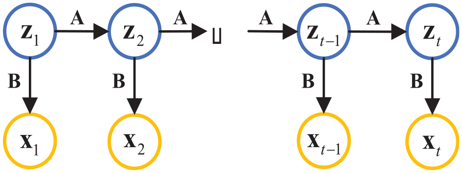
Linear dynamic latent variable.
The formal definition of the LDLV model is given below:
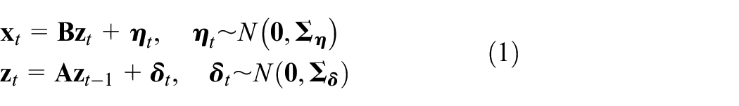
where
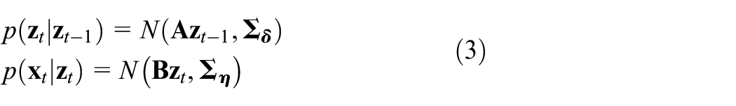
The joint probability of LDLV model can be formulated as follows:
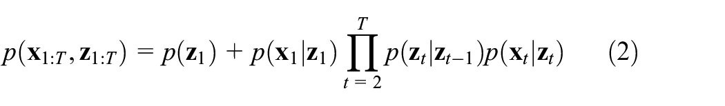
where the probability distribution of the latent variable at the initial time is a Gaussian distribution, and the prior density
The EM algorithm is used to estimate the parameters
Fault detection and classification using ASLDLV
ASLDLV model
The ASLDLV model is an extension of the LDLV model by introducing a series of switching variables to the LDLV model framework. The ASLDLV model can be seen as a combination of a hidden Markov model with a linear dynamic system, which not only describes the dynamics among samples but also describes the dynamics of multiple models. Compared with the SLDS model, the ASLDLV model uses an augmented dynamic switching transition matrix as the transition matrix. The introduction of the augmented dynamic switching transition matrix considers not only the switching variables at the previous moment but also the latent variables at the last sample. It means that the ASLDLV model can contain the high-order dynamic characteristics of multiple sub-models. The structure of ASLDLV model is illustrated in Figure 2.
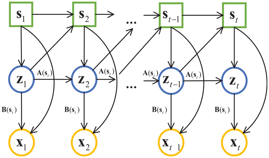
Augmented switching linear dynamic latent variable model.
The ASLDLV model can be described as follows:
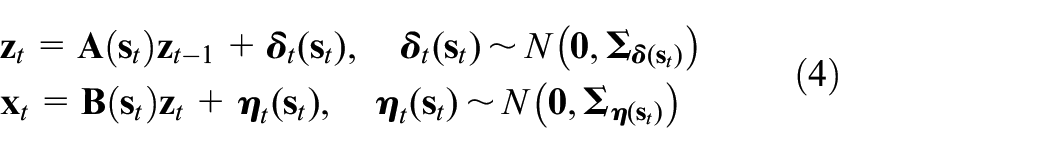
where
For ASLDLV model, the switching variable

The initial switch variable distribution

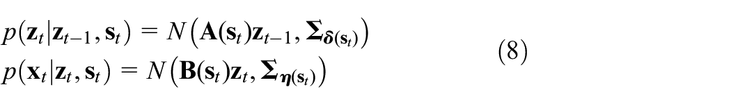
The ASLDLV model defines a joint distribution
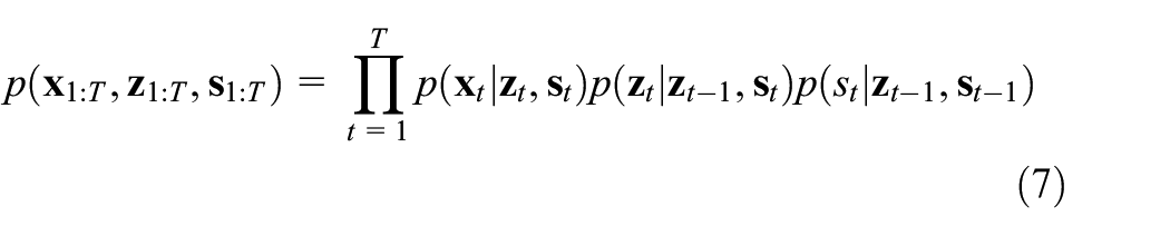
where
In summary, the ASLDLV model is determined by the parameter set:
Training ASLDLV parameter
First, the EM algorithm can be used to estimate the parameters of all the single LDLV models, and the detailed derivation is reflected in the Appendix A. Then, the Gaussian forward filtering method is used to estimate the augmented dynamic switching transition matrix
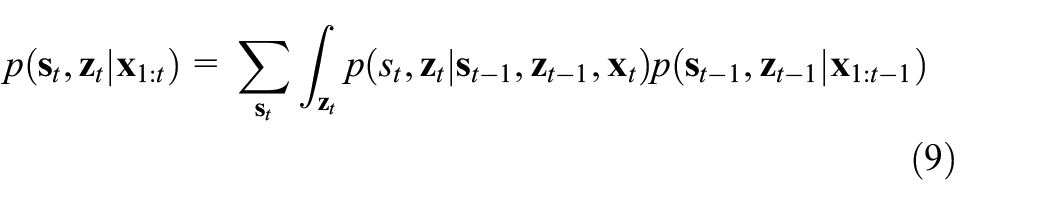
But the exact filtered inference in the ASLDLV model is intractable. At the first time, is an indexed set of Gaussians. At the second time, due to the summation over the states,
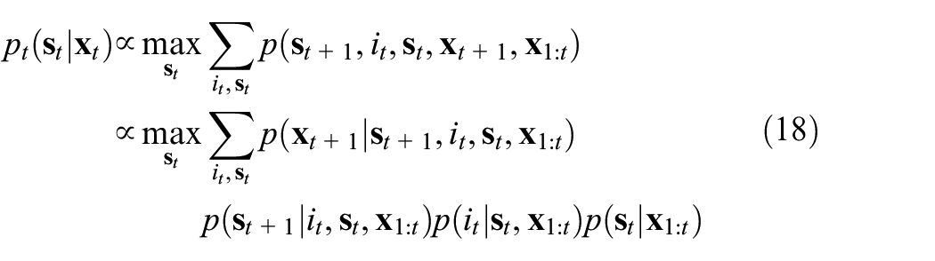
Here, the approximate recursion of Equation (9) can be shown as follows:

where
where
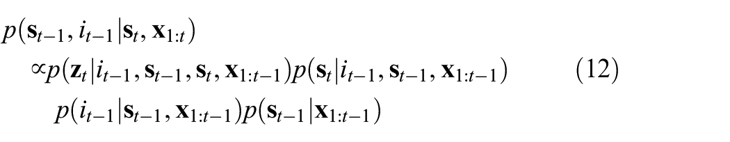
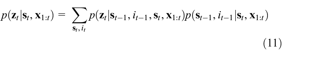
The first factor in Equation (12),

where the augmented dynamic switching transition matrix
Fault detection and classification based on ASLDLV
After the ASLDLV model is built, an important parameter, posterior probability, can be calculated based on ASLDLV model. The posterior probability reflects the attribution of samples to different modes. Therefore, it can effectively isolate the fault samples from the normal samples and distinguish different fault modes. In this paper, the posterior probability is flexibly applied for fault detection and fault classification. For a test sample

Comparing the statistics

where
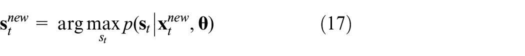
Furthermore, fault classification based on ASLDLV model can be conducted by finding out the maximum of all the posterior probabilities of the current test sample relative
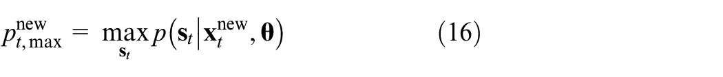
where
Therefore, the current sample belongs to the mode with the maximum posterior probability.
In Equations (14) and (16), the posterior probability of the current time is essentially a mixture of Gaussian distributions. Therefore, it can be approximated with a limited
The detailed procedures of fault detection and classification based on ASLDLV model can be summarized as follows:
Collected training data set including the normal data set
Build the ASLDLV model using the normal training data set
For a test sample
For fault classification, build the ASLDLV model using the normal data set
Train the ASLDLV model for fault classification based on the algorithm in section “Training ASLDLV parameter” to obtain
(6) For a test sample
The schematic diagram of fault detection and fault classification based on ASLDLV model is shown in Figure 3.
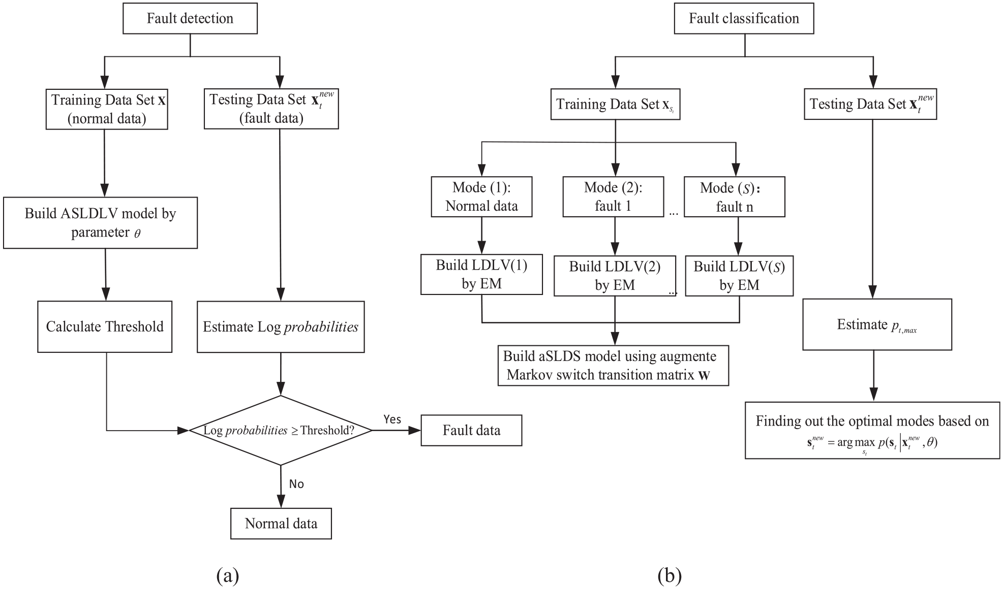
The flow chart of fault detection and classification based on ASLDLV.
Tennessee Eastman process simulation
In order to verify the performance of the established model, the simulation will perform fault detection and classification under the influence of a high-intensity dynamic process and random factors. Therefore, this paper chooses the Tennessee Eastman (TE) process for simulation research. TE process is a benchmark simulation based on a real industrial process. It has been widely used as a bed of continuous process for fault detection and classification. The process consists of five major units: a reactor, a product condenser, a separator, a recycle compressor and a product stripper. The flow chart of TE process is shown in Figure 4.
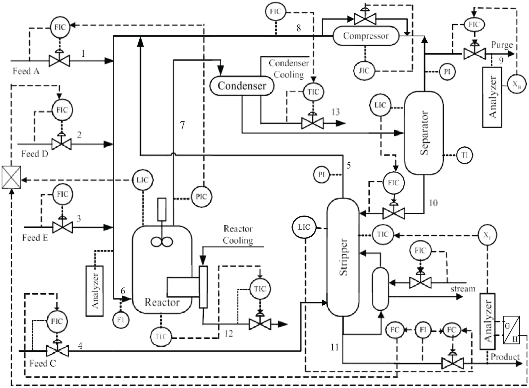
The flow chart of TE industrial process.
In this section, the proposed ASLDLV model is applied to TE process to achieve fault detection and fault classification. We focus on how to deal with dynamic, uncertain, and multimode problems to demonstrate the performance of fault detection and classification. There are 41 measurement variables and 12 operating variables for TE process. In this paper, 16 variables are selected for fault detection and classification, which are A feed, D feed, E feed, A and C feed, recycle flow, reactor feed rate, reactor temperature, purge rate, product separator temperature, product separator pressure, product separator underflow, stripper pressure, stripper temperature, stripper steam flow, and reactor cooling water outlet temperature. The normal data and seven different fault modes are used for case studies, which are A/C feed ratio, B component unchanged, B component, A/C feed ratio unchanged, A Feed loss, inlet temperature of condenser cooling water, response dynamics, reactor cooling water valve, and unknown.
For fault detection, a normal data set including 500 samples are used as training data set. A total of 960 samples for each fault mode is collected as test data. For each fault testing set, the faults are introduced after the 160th sample. The control limit can be determined when the significance levels are 0.01. The results of fault detection using the logarithm of posterior probabilities, denoted as the log probabilities, based on the ASLDLV method for seven fault modes are given in Figure 5.
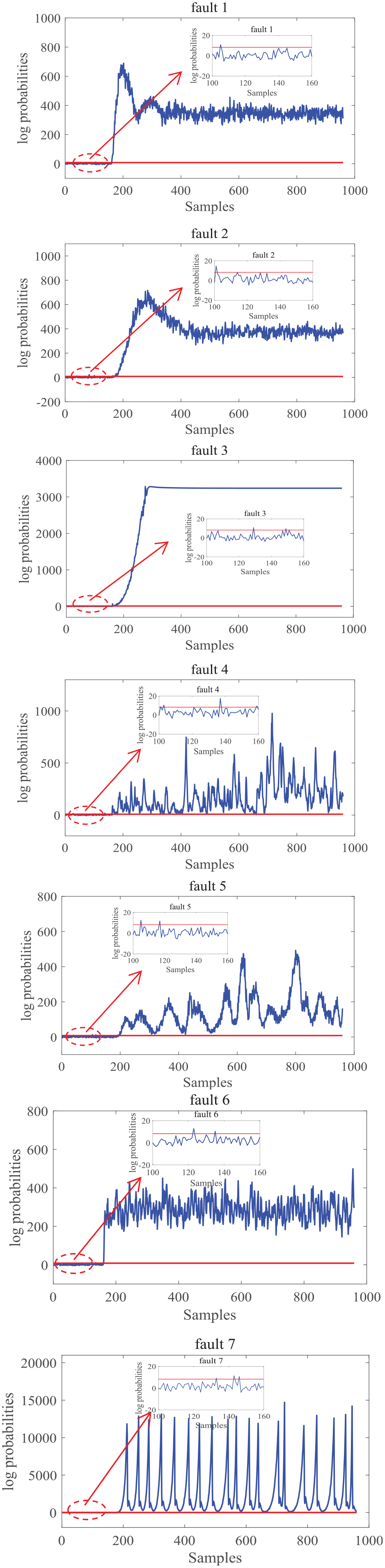
The results of fault detection based on the ASLDLV.
In Figure 5, it can be seen that the log probabilities corresponding to the seven fault modes all exceed the control limit about the 160th sample point, with a low false alarm rate and missing alarm rate. The detailed performance of fault detection is listed in Table 1.
The performance of fault detection based on ASLDLV.
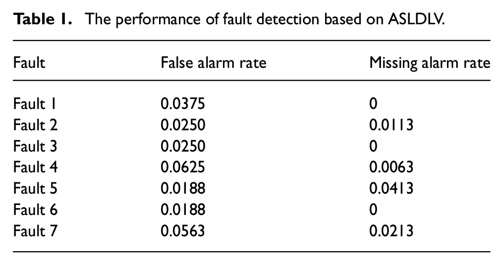
From Table 1, it is not difficult to find that the log probabilities have no delay for fault 1, 3, and 6. Also, fault 2, 4, 5, and 6 have a slight delay with 9, 5, 33, and 17 samples, respectively, when the fault first occurs. In addition, the false alarm rate of all fault is less than 0.0625. It can be seen that the ASLDLV algorithm takes into account the multifeature interaction of the data. Even if it is exposed to an industrial environment with strong dynamics and uncertain factors such as noise, the model can still identify the occurrence of faults well.
Besides dynamic and uncertain underlying data, ASLDLV model can extract dynamic characteristics among multiple models. To demonstrate such a superior ability of ASLDLV model, the single fault classification and the multiple fault classification using ASLDLV method are performed, respectively. As mentioned in above, seven fault data are collected. In this paper, each fault training set includes 480 samples, with the first 20 samples of each fault being normal and the remaining samples being faulty. For single fault classification, the normal data and each fault training data are used as the training set to build ASLDLV model. Then, both 960 normal samples and each fault data sets including 960 samples are applied to test the performance of fault classification. The specific results of fault classification for seven different faults are shown in Figure 6.
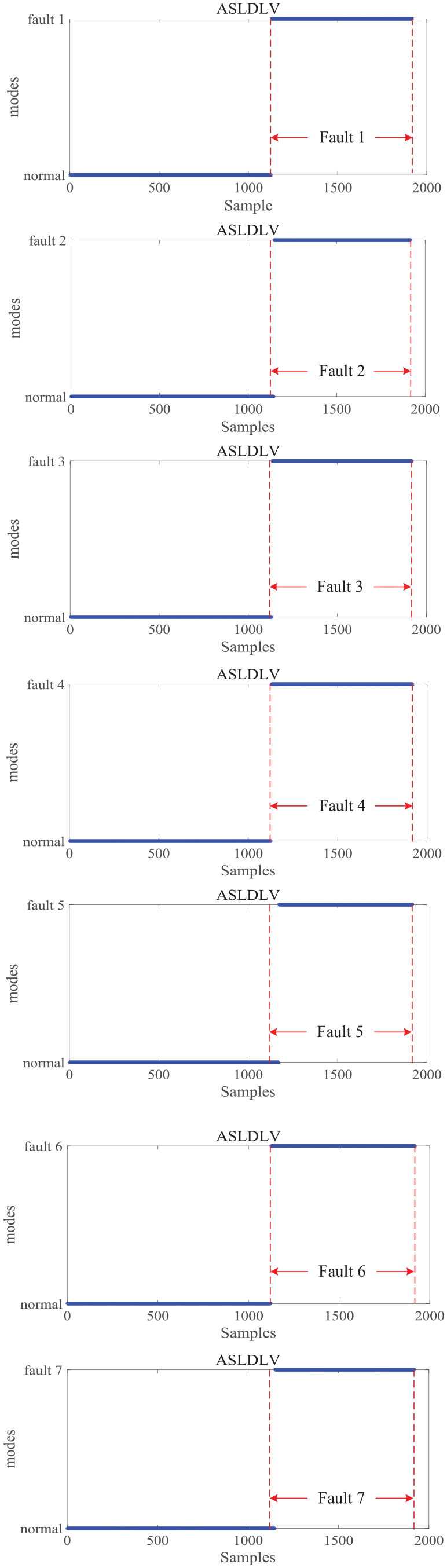
Fault error rate based on ASLDLV.
In Figure 6, the range of red dotted line is the correct classification range, and the blue line segment is the actual classification result. It can be clearly seen that the normal mode and fault mode can be clearly classified for seven faults. Also, there are only a small number of misclassified samples appear during the transition from normal to fault. It shows that accurate attributes of samples can be obtained by finding out the maximum posterior probability value. In order to demonstrate the classification performance of ASLDLV model, the misclassification rate is calculated and compared with the SLDS, LDS, and SVM methods. The specific comparison results are shown in Table 2.
Fault classification error rate based on ASLDLV.
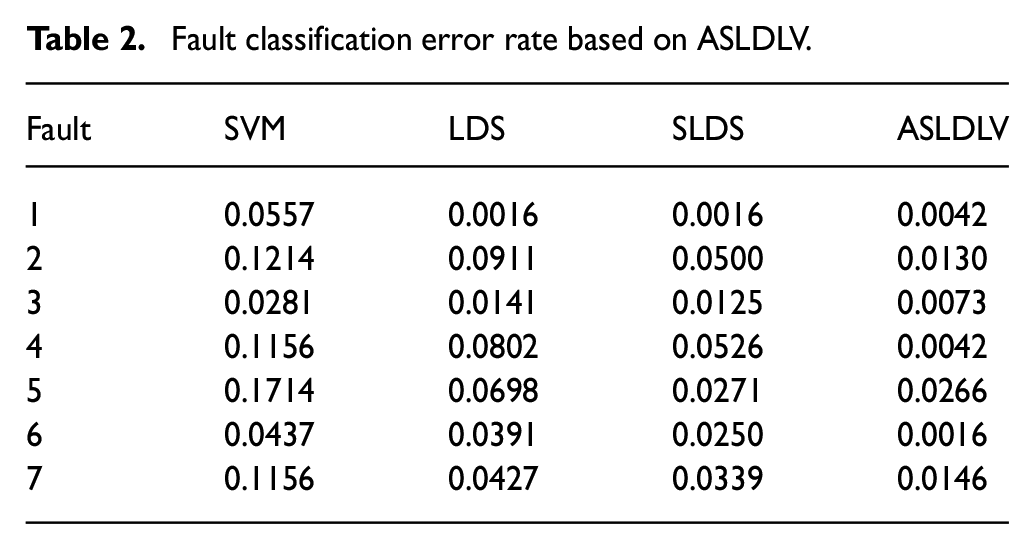
From Table 2, it can be observed that the ASLDLV model has the lowest error rate of classification for fault 2 to 6, except for fault 1. Also, the classification error rate of the ASLDLV model for fault 2 to 6 significantly lower than the other methods. This improvement can be attributed to the introduction of the augmented transition matrix, which enables the ASLDLV model to not only capture multiple features among the process data but also mine high-order information between multiple models. Therefore, the results of fault classification using ASLDLV model are more accurate.
To more deeply evaluate the ability of the ASLDLV model in handling the dynamic correlation of multiple models, the multiple fault classification is further carried out. In this section, both the normal data and seven faults are used as the training set to build a new ASLDLV model. Then, a test set including 960 normal samples and seven fault samples (7 × 960 = 7680) is used for test the performance of fault classification. It should be noted that the test set of 8 data modes is arranged in order of normal samples, fault 1 to fault 7 and each fault is introduced after 160th sample time. The results of fault classification based on ASLDLV method are shown in Figure 7. At the same time, the results of fault classification based on several comparing methods such as SVM model, LDS model and SLDS model are also given in Figure 7.
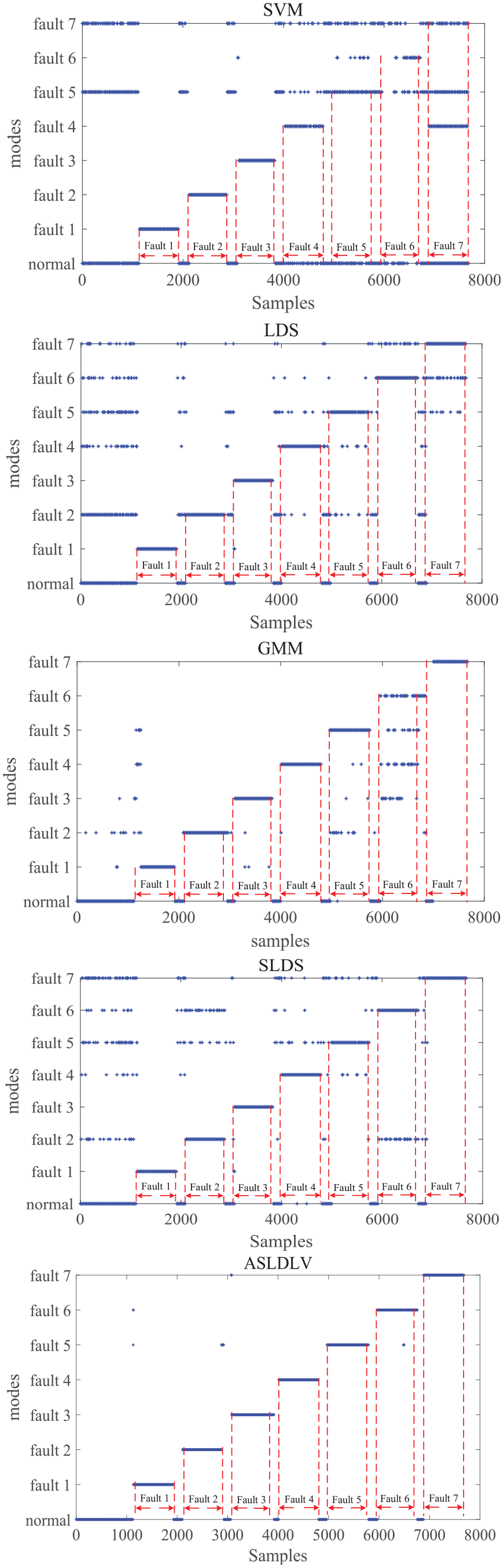
Fault diagnosis diagrams.
In Figure 7, the abscissa represents the sampling point and the ordinate represents the data modes including normal mode and fault mode from one to seven. Also, the location of the blue dot represents the mode that the corresponding sample belongs to. For test samples, the samples are arranged in the continuous order from mode 1 to mode 8. Each mode contains 960 samples, and the fault is introduced at the 161th sample point. From Figure 7, it can be seen that the classification results of SVM model have false classification for each mode, especially for fault 5 mode, fault 6 mode, and fault 7 mode. Compared to the SVM model, the LDS model has shown an improved classification effect of the above fault modes, because the LDS model can extract the dynamic and uncertainty characteristics of the process data, while the SVM model is a static model. Therefore, the LDS model can classify most of the samples into the corresponding eight modes accurately. Although the LDS model can deal with the dynamic characteristics of the data, in the fault classification of multiple modes, the LDS model cannot extract the multimode characteristics, which leads to the weakening of the characteristics between modes. Since the first 160 samples of each mode are normal data, the posterior probability of switching mode from fault data to normal data will fluctuate greatly, so the normal data are misjudged as fault data by LDS model. Thus, the classification effect is unsatisfactory when dealing with multiple modes. The Gaussian Mixture Module (GMM) model establishes multiple Gaussian distributions by analyzing the feature data under different modes, and effectively processes the multimode feature information. It can be seen from Figure 7 that the GMM model is superior to the LDS model in the division of normal data. The SLDS model improves the problem of multimode feature extraction on the basis of the LDS model. Compared with the three methods mentioned above, the SLDS model in addition to improving the overall classification effect, and also improves the classification accuracy of normal data, fault 6 and fault 7. Therefore, in the case of multiple faults, the mining of multimode feature is very important. However, the transition matrix used in the SLDS model during the mode switching process only considers the random probability model, which cannot mine deeper feature information. The ASLDLV model proposed in this paper utilizes an augmented dynamic switching transition matrix as the transition matrix between modes switching, which can mine high-order feature information and improve the accuracy of fault classification greatly. The ASLDLV model demonstrates higher accuracy in classifying the eight modes, with only a minimal number of misclassified samples. Specifically, for fault 4, the ASLDLV model misclassifies 15 samples as normal mode, while the SLDS model misclassifies 23 samples as normal mode, fault 5 mode, fault 6 mode, and fault 7 mode. Regarding fault 7, the ASLDLV model misclassifies 5 samples as normal mode, while the SLDS model misclassifies 11 samples as normal mode and fault 5 mode. These results clearly indicate that the ASLDLV model exhibits superior fault classification performance, particularly in scenarios involving multiple fault modes. Furthermore, the specific false alarm rate and misclassification rate are summarized in Table 3.
False alarm rate and misclassification rate based on four methods.
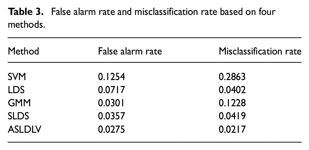
From Table 3, it can be seen that the misclassification rate of ASLDLV is 0.0217, and the False alarm rate is 0.0275. Both of two indicators are the lowest among the compared methods. This may depend on that the ASLDLV method is able to simultaneously consider dynamic, uncertain, and multimode characteristics relative to the SVM model and LDS model. From Table 3, it can be seen that the GMM model has a good classification result for normal data, which is because the GMM model can effectively process multimode feature information. At the same time, due to the lack extraction of other features of process data, the GMM model has a poor classification effect when classifying the fault data. The SLDS method has a good classification performance, it is because the dynamic features of different LDS models are further considered. Similarly, it is obvious ASLDLV model performs better classification performance. It is not difficult to infer that the extraction of higher-order dynamic information, based on ASLDLV model, plays an important role, which the performance of fault classification is greatly improved. Therefore, these results can effectively prove that the ASLDLV model using the augmented dynamic transformation matrix as the modal switching transformation matrix can achieve effective results in the practical application of fault classification in the actual industrial process with dynamic, uncertainty, and multimodality.
Conclusion
In this paper, a new augmented SLDS model which can simultaneously extract the dynamic, uncertain, and multimode is proposed for fault detection and classification in complex industrial processes. In the simulation of the Eastman process in Tennessee, the model proposed in this paper is exposed to highly dynamic, complex uncertainties and multiple fault types. The results show that ASLDLV model has better performance in fault detection and fault classification. For fault detection, ASLDLV algorithm uses the logarithm of posterior probability as new statistics to successfully achieve fault detection. Also, the results of fault detection show the great monitoring performance. Furthermore, comparing the ASLDLV model with the SVM model, LDS model and SLDS model, the results of fault classification can further demonstrate superior ability of classification, especially for multiple fault classification. This not only attributes to the extraction of multiple process feature. It is more important that dynamic information of higher order among multiple models can be mined by constructing the augmented dynamic switching transition matrix, so that the most suitable mode of samples can be more accurately found.
However, the method proposed in this paper is also conservative in some aspects. For example, the algorithm proposed in this paper has the best fault diagnosis effect for the six selected fault types, and the classification effect of other fault types may be poor. In future research, more types of faults will be considered for effective detection and classification. In addition, the transition between modes will be considered. In actual industry, the switch of process modes including fault modes is not sudden, while there is a transition between modes. However, process characteristics in the transition is complex, which can lead to poor performance of fault classification. Therefore, how to identify the transition sample and give a soft classification result will be further studied in the future.
Footnotes
Appendix A
Declaration of conflicting interests
The author(s) declared no potential conflicts of interest with respect to the research, authorship, and/or publication of this article.
Funding
The author(s) disclosed receipt of the following financial support for the research, authorship, and/or publication of this article: This work was supported in part by the National Natural Science Foundation of China (NSFC) under Grant 62273242 and the Natural Science Foundation of Liaoning Province (2023-MS-242).
Data availability statement
Data sharing not applicable to this article as no datasets were generated or analyzed during the current study.