
Abstract
With the advancement of modern industrial technology, square composite tubes have seen increasing application across various critical engineering fields. Traditional square steel and aluminum tubes are being progressively replaced by high-strength, corrosion-resistant composite alternatives. Robotic filament winding has become the dominant manufacturing approach due to its multi-degree-of-freedom (DOF) flexibility and high-precision control, which significantly enhance production efficiency and product quality. However, conventional obstacle-avoidance strategies based on path–velocity decomposition often fail to simultaneously satisfy dynamic feasibility and strict collision constraints, leading to suboptimal performance. To address this issue, this study proposes a unified optimal control framework for obstacle-avoiding trajectory planning in filament winding robots. The formulation integrates robot dynamics, joint constraints, collision-avoidance requirements, and time-optimal objectives within a pseudospectral transcription scheme. The resulting nonlinear programming problem is solved efficiently using automatic differentiation and numerical optimization techniques. Simulation studies conducted on a 6-DOF industrial robot demonstrate that the proposed approach generates dynamically feasible and smooth trajectories under constrained winding environments. Comparative evaluations against both a traditional industrial planning strategy (Rapidly-Exploring Random Trees (RRT)–Artificial Potential Fields (APF)–polynomial) and an optimization-based method, Covariant Hamiltonian Optimization for Motion Planning (CHOMP), indicate improvements in trajectory duration and jerk energy while maintaining strict dynamic and collision constraints.
Keywords
Introduction
With the rapid advancement of modern industrial technology, square composite pipes (square tubes) have been increasingly employed as structural components in various critical sectors, including aerospace (Dinită et al., 2023), automotive (Zhang et al., 2020), and new energy systems (Wang et al., 2025; Zu et al., 2018). Traditionally, square tubes were primarily fabricated from square steel or aluminum alloys. However, steel tubes are heavy and exhibit poor corrosion resistance, while aluminum alloy tubes, although lightweight and corrosion-resistant, are prone to oxidation and suffer from poor performance at low temperatures (Alabtah et al., 2021b). As a result, these traditional materials are gradually being replaced by high-strength, corrosion-resistant, and mildew-proof composite square tubes (Alabtah et al., 2021a; Zhang et al., 2024). Currently, the main forming methods for square tubes include hot rolling, cold rolling, welding, and filament winding (Han et al., 2020). Hot-rolled tubes tend to suffer from poor surface quality and low-dimensional accuracy, while cold rolling is limited in formability, and welded tubes often exhibit inconsistent quality and internal defects. In contrast, filament winding has emerged as the mainstream technique, particularly for composite square tubes, due to its flexibility, high material utilization, and capability to produce lightweight, high-strength components (Yadav et al., 2025).
Research on robotic motion planning with obstacle avoidance has mainly progressed along several directions. Geometry-based search methods, such as improved A* algorithms combined with artificial potential fields (Tang et al., 2024), are capable of generating collision-free paths in joint space (Chen et al., 2023); however, these approaches often neglect robot dynamics, making the resulting trajectories difficult to execute accurately or inefficient in practice. Polynomial interpolation-based trajectory planning methods (Hu et al., 2023) can produce smooth trajectories, but their optimization capability and real-time performance are limited when dealing with complex obstacles and dynamic coupling. Optimization-based methods, which reformulate obstacle avoidance as a trajectory optimization problem (Li et al., 2023), offer a more systematic framework. Nonetheless, jointly addressing time-optimality, complex dynamics, and strict collision constraints remains a significant challenge. Particularly, traditional path–velocity decomposition approaches suffer from inconsistency in performance metrics between path planning and trajectory generation subproblems, typically resulting in suboptimal solutions that fail to satisfy the stringent requirements of high speed, smoothness, precise obstacle avoidance, and robot physical limitations (LaValle, 2011; Liu et al., 2023; Pham, 2014).
To address the above challenges, this study formulates the obstacle-avoiding trajectory planning problem in robotic filament winding as a unified time-optimal control problem. The main contributions of this work are summarized as follows:
A unified time-optimal control formulation for filament winding robots is developed. Unlike conventional path–velocity decomposition strategies, the proposed framework integrates robot dynamics and collision-avoidance constraints associated with pin structures mounted on the winding mandrel into a single optimization formulation, enabling dynamically feasible trajectory generation under constrained conditions.
An optimized numerical solution framework is constructed to enhance the computational efficiency and stability of the pseudospectral transcription. By introducing persistent data caching and reorganizing decision-variable structures, the computational burden associated with the Jacobian evaluation is reduced, and the convergence behavior of the nonlinear programming (NLP) solver is improved accordingly.
Optimal control algorithm
To clearly present the proposed control method, this section provides a systematic formulation of the optimal control problem and its numerical solution procedure. Optimal control aims to determine the control input that minimizes or maximizes a given performance index under specific system constraints (Bryson, 2018; Bordalba et al., 2022). Formally, it seeks an extremum of a performance functional defined in terms of the system states and control inputs, subject to the equations of motion and admissible bounds.
In this study, the optimal control method is systematically formulated and implemented for the trajectory optimization of a 6-DOF filament winding robot. The problem formulation includes a time-minimization cost function with a smoothness regularization term, dynamic equations derived from the Newton–Euler model, path constraints incorporating joint limits and collision avoidance, and boundary conditions defined by initial and target configurations.
The continuous-time problem is then transcribed into an NLP formulation using the pseudospectral method, where Chebyshev–Lobatto nodes are employed for efficient discretization. The NLP is solved via an interior-point method supported by automatic differentiation (AD), ensuring high computational efficiency and numerical precision. The complete procedure—from problem formulation to numerical solution and simulation validation—is summarized in Figure 1, and each component is elaborated in the following sections.
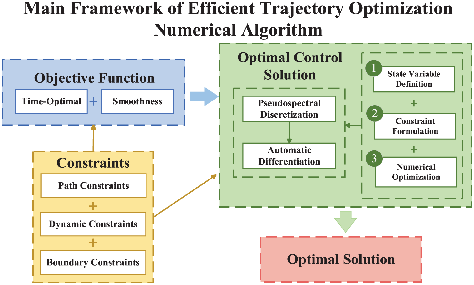
Framework of the efficient numerical method for time-optimal trajectory planning.
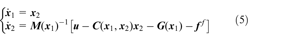
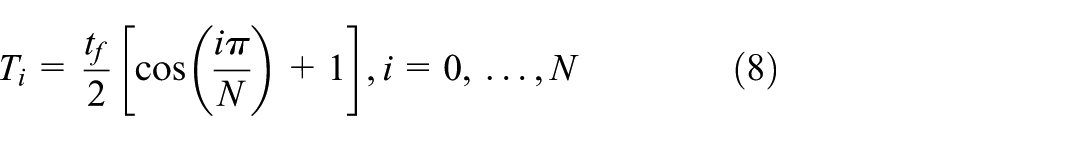
Since the subject of this study is a 6-DOF robot, the positions and velocities of its six joints are selected as the state variables, while the joint torques serve as the control variables. The dynamic state of the robot can therefore be defined as follows:
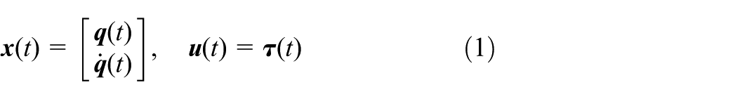
In the equations,
Cost function
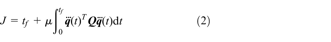
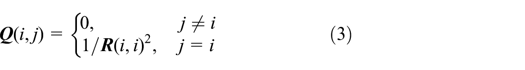
The cost function serves as the objective function used to identify the optimal solution. To enhance the operational efficiency of the manipulator, this study adopts a time-minimization strategy by selecting the total motion duration as the primary cost. The overall cost function is defined as the sum of the final time and a regularization term designed to promote naturalness and smoothness of the generated trajectory:
here,
where
The parameter μ is a non-negative weighting coefficient used to balance time-optimality and trajectory smoothness. In this study, μ is selected as a small positive constant (
Dynamic constraints
The dynamic equations of the robot can be derived from the Newton–Euler formulation as follows:

In this formulation, where
Let
Accordingly, the dynamic equations can be rewritten as:
Path constraints
The path constraints include limitations on joint position, velocity, acceleration, torque, and torque rate, as well as collision-avoidance conditions. These can be formulated as:
Joint position constraints:
Joint velocity constraints:
Joint acceleration constraints:
Torque constraints:
Torque rate constraints:
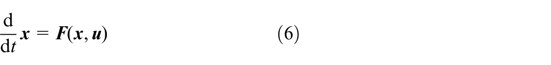
In addition to the physical limitations of each robot joint, the path constraints must also ensure collision avoidance. To simplify the formulation, both the robot and obstacles are approximated as sets of spheres, allowing for efficient manual estimation. Specifically, the manipulator is approximated using M spheres to represent its joints and links, while the obstacles—namely the pin-like structures on the mandrel during the filament winding process—are approximated using V spheres. Let

Sphere-based approximation of the robot and obstacles.
In addition, the workspace boundaries also need to be constrained. Let
Lower workspace bounds:
Upper workspace bounds:
Boundary conditions
For a 6-DOF manipulator, the boundary conditions for motion trajectory planning refer to the initial and final conditions, including:
Initial and final positions:
Initial and final velocities:
Initial and final accelerations:
Final time:
here,
Efficient numerical algorithm for trajectory optimization
The objective of trajectory optimization is to generate motion trajectories with optimal characteristics while satisfying all imposed constraints. Numerical methods for trajectory optimization have been extensively reviewed by Bordalba et al. (2022) and Chai et al. (2023). A standard approach involves transcribing the continuous time-optimal control problem into a discretized optimization problem, solving it using an optimization solver, and then reconstructing an approximate solution to the original continuous-time problem via polynomial interpolation.
Two key components that play a critical role in numerical trajectory optimization are transcription and optimization. By improving the performance of these two components, a more efficient implementation can be achieved. In this study, the continuous time-optimal control problem is transcribed using a pseudospectral method, and the resulting discretized problem is solved using an interior-point method equipped with AD.
Pseudospectral discretization for optimal control
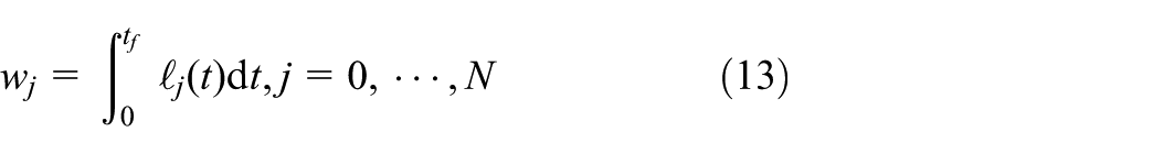
In the optimal control problem of robotic trajectory planning, the decision variables include
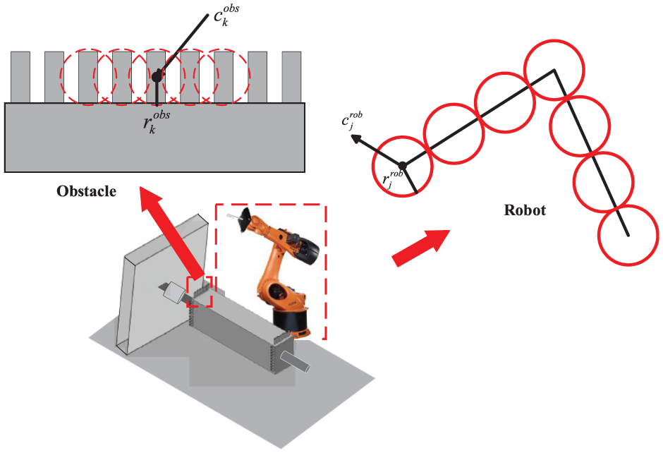
The first step is the selection of nodes. In the pseudospectral method, nodes are usually chosen as the roots of orthogonal polynomials. In this study, the Chebyshev orthogonal polynomials are adopted due to their computational simplicity and efficiency in node calculation. Specifically, the Chebyshev–Lobatto points are selected as the collocation nodes. For
Polynomial interpolation in the pseudospectral method can be implemented using barycentric interpolation. The barycentric form can be expressed as a linear combination of Lagrange polynomials. Accordingly, the state trajectory and control trajectory can be represented as:
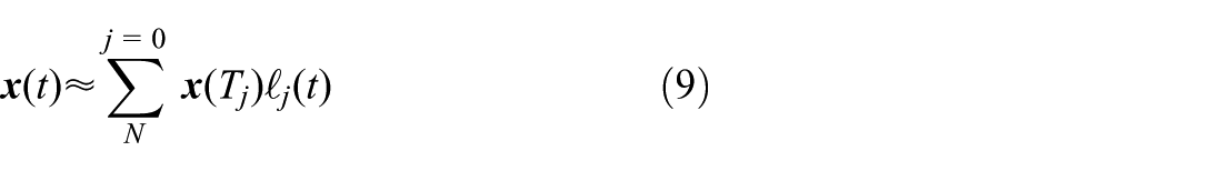
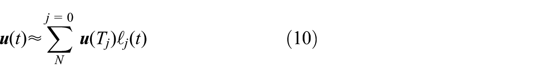
here,
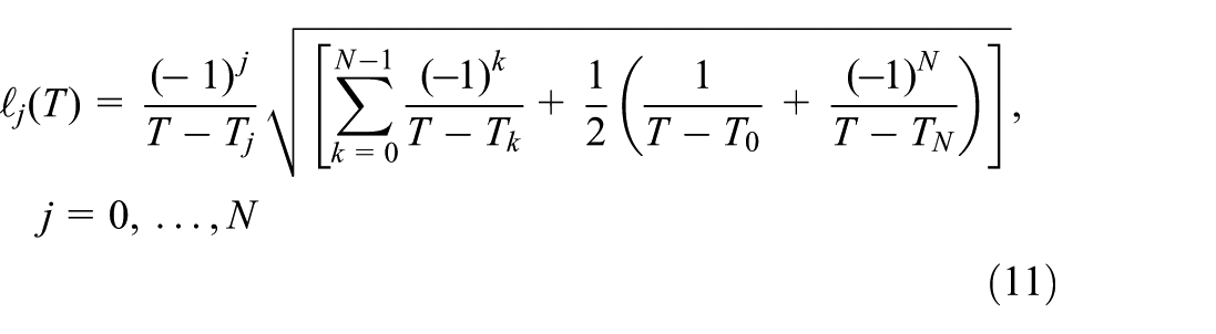
The function
where
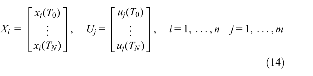
Let the state and control variables at collocation nodes be denoted as:
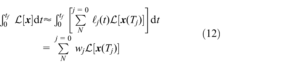
The dynamic constraints are formulated as:
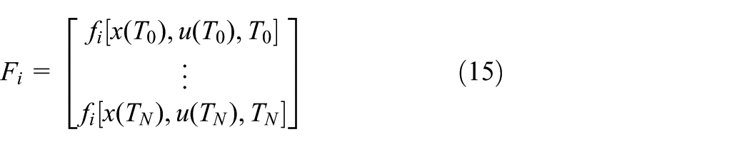
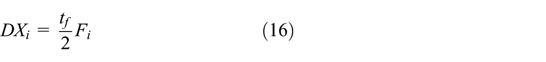
where D is the differentiation matrix that computes the scaled time derivative of the polynomial approximation of
AD
Almost all machine learning algorithms, during training or inference, can be formulated as optimization problems. When the objective function is differentiable, the problem reduces to finding a stationary point of the training function. In most cases, closed-form solutions of such stationary points are unavailable, and numerical optimization algorithms—such as gradient descent, Newton’s method, and quasi-Newton methods—must be employed. These algorithms all rely on the evaluation of first- or second-order derivatives, including the gradient and the Hessian matrix. Numerical differentiation is computationally expensive and prone to round-off and truncation errors. Symbolic differentiation may also introduce inaccuracies, especially when computing higher-order derivatives like the Hessian.
AD, also known as algorithmic differentiation, is a generalization of the backpropagation algorithm that computes exact derivatives of differentiable functions at specific points (Baydin et al., 2018). AD is particularly designed to compute the derivatives, gradients, and Hessians of complex functions—often structured as multi-layer compositions—with both high accuracy and computational efficiency. Unlike traditional finite difference methods, AD does not rely on step-size parameters, and it enables exact gradient computation without numerical approximation errors (Bolte and Pauwels, 2021). Due to its modular structure and ease of implementation, AD has been widely integrated into various software tools across programming languages. Examples include CppAD for C++ and CasADi for MATLAB. CasADi is adopted in this work due to its excellent usability for numerical optimization, particularly for optimal control problems in the MATLAB environment (Andersson et al., 2012, 2019).
An articulated body refers to a system of multiple rigid bodies connected by joints, allowing relative motion along certain DOFs. Since the computational cost of AD is proportional to that of function evaluation, the articulated-body algorithm (Featherstone, 2008) is employed in this study to efficiently estimate the robot dynamics.
Numerical optimization framework
To further improve the computational efficiency and solution stability of time-optimal trajectory optimization, the pseudospectral optimization framework was restructured and enhanced in this study, with additional adjustments tailored to the performance characteristics of CasADi and the IPOPT solver. The overall structure is illustrated in Figure 3.
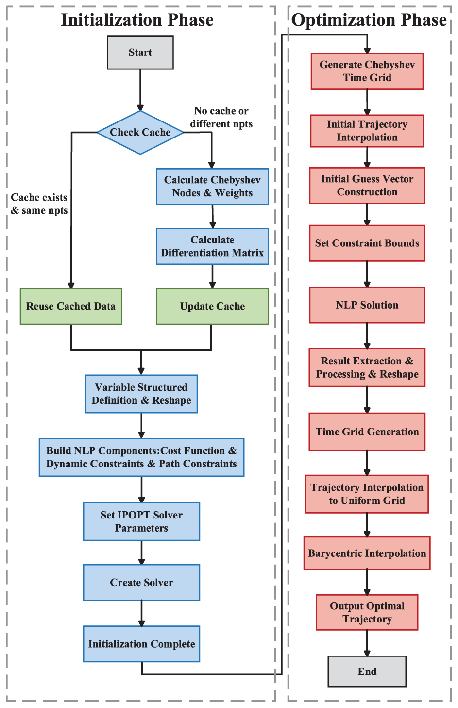
Structural flowchart of the time-optimal trajectory planning method.
In traditional pseudospectral methods, Chebyshev nodes, weights, and differentiation matrices are recalculated at each initialization stage, leading to substantial computational overhead. In this study, a persistent caching mechanism is introduced to reuse previously computed data when the number of nodes remains unchanged, thereby avoiding redundant calculations and significantly reducing initialization time.
The decision variable x is structurally decomposed into state variables X, control variables U, and final time using matrix reconstruction. This structured representation minimizes indexing errors, facilitates program readability and future extensions, and enhances compatibility with the CasADi framework for efficient AD.
For initial trajectory interpolation, a linear interpolation method combined with an extrapolation strategy (“linear” + “extrap”) is employed. This prevents the generation of NaN values when Chebyshev nodes exceed the specified time range, thereby improving the stability and feasibility of trajectory initialization.
In terms of solver configuration, several key IPOPT parameters are carefully tuned (Wächter and Biegler, 2006). The robust sparse linear solver MUltifrontal Massively Parallel sparse direct Solver (MUMPS) is employed, and the interior-point method is configured with an adaptive barrier strategy to improve convergence speed and numerical stability (Amestoy et al., 2001). Termination tolerances are balanced to ensure both fast convergence and solution feasibility. A limited-memory Hessian approximation is enabled to strike a balance between accuracy and computational cost while avoiding excessive memory usage.
Through these structural improvements, the overall implementation not only achieves higher computational efficiency but also enhances adaptability to complex dynamics modeling of multi-DOF robotic systems, making it well-suited for practical engineering applications.
Efficient trajectory optimization: Simulation study
Simulation setup
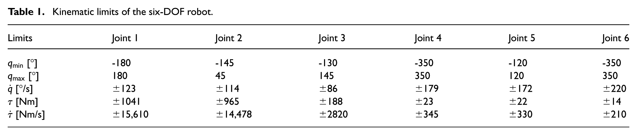
To validate the proposed method, simulations are conducted using a 6-DOF industrial robot. Specifically, the robot model adopted is the KUKA KR 160 R1570 NANO. The robot is required to complete a collision-free trajectory within a constrained workspace. The joint limits of the six-axis robot are listed in Table 1, and the robot’s links and surrounding obstacles are approximated as spheres, as shown in Figure 4(a).
Kinematic limits of the six-DOF robot.
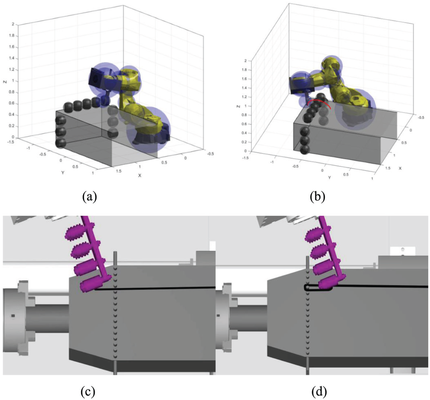
Visualization of robot modeling, obstacle-avoidance trajectory planning, and winding motion simulation. (a) Initial robot-obstacle configuration. (b) Optimized obstacle-avoiding trajectory. (c) Winding simulation before obstacle avoidance. (d) Winding simulation after obstacle avoidance.
It should be noted that the obstacles considered in this study correspond to pin structures mounted on the winding mandrel to guide and control the fiber path during the filament winding process. Their spatial distribution is determined by specific process requirements rather than by arbitrary density settings. Therefore, unlike general mobile robot navigation problems, the obstacle configuration reflects practical manufacturing constraints instead of artificially generated cluttered environments. Nevertheless, the proposed optimization framework can accommodate different obstacle layouts and constrained workspace configurations without structural modification.
The trajectory optimization algorithm is based on the previously introduced pseudospectral method, integrated with CasADi and the IPOPT solver, and implemented in the MATLAB environment. The optimization objective is to minimize the time required for the robot to complete a specified trajectory while ensuring trajectory smoothness and satisfying all system constraints.
The winding process is simulated as illustrated in Figure 4(b). The resulting simulations produced time-optimal trajectories that successfully guided the robot through constrained environments. The robot successfully avoids obstacles and accurately reaches the target position from the initial state, thereby demonstrating the feasibility of the proposed method.
The proposed method is implemented in simulation using KUKA Sim 4.3, which allows the visualization of obstacle-avoiding trajectories during the winding motion. As shown in Figure 4(c) and (d), the robot successfully performs the winding operation around a square mold.
Comparative analysis of the improved method
To verify the effectiveness of the proposed numerical optimization structure, we compare the initialization time, solver time, and trajectory duration before and after the improvements under different numbers of discretization nodes. The simulation results are shown in Figure 5(a) to (c).
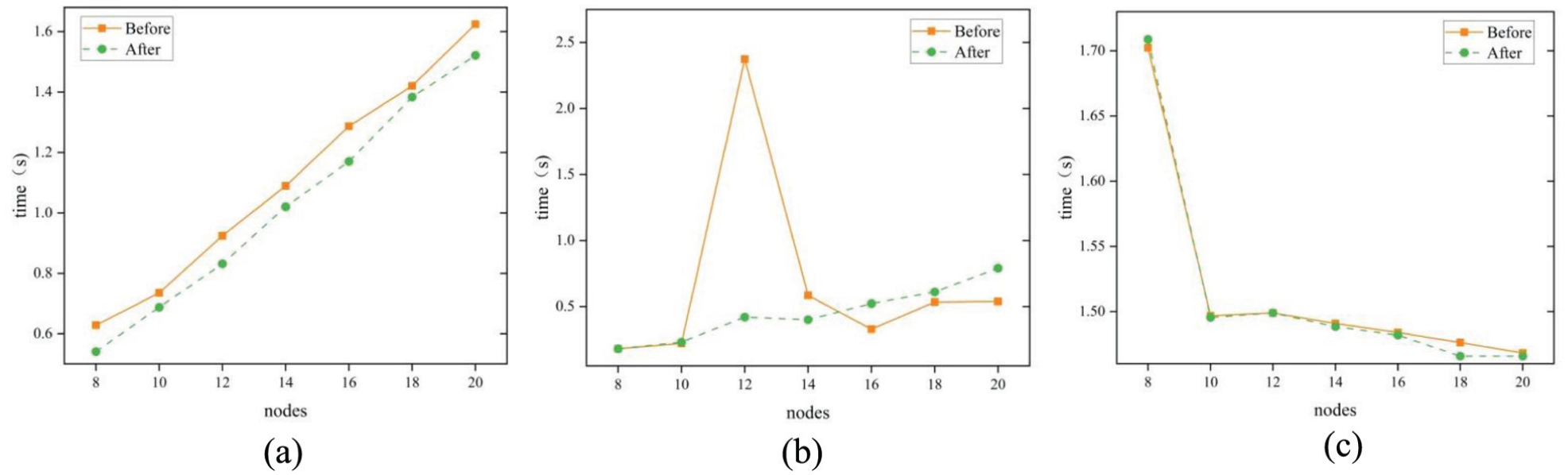
Effect of node number on (a) initialization time, (b) solver time, and (c) trajectory duration.
As illustrated in Figure 5(a), the initialization time increases with the number of nodes in both cases; however, the improved method consistently exhibits a lower initialization time than the original version. For instance, when the number of nodes reaches 20, the initialization time is reduced from 1.62 seconds to 1.52 seconds, achieving a 6.2% decrease. Moreover, the improved version maintains low latency across all tested node configurations, indicating good numerical scalability.
Figure 5(b) compares the solver times of both implementations. The original method exhibits a sudden spike in computation time at 12 nodes, indicating unstable convergence. This phenomenon is mainly caused by poor scaling and a dense Jacobian structure, which reduces the line-search step acceptance in IPOPT and leads to irregular convergence behavior. In contrast, the improved method eliminates such instability by employing structured variable grouping and gradient-based scaling, consistently maintaining the solver time within 0.78 seconds under the same initial conditions. These enhancements demonstrate that the combination of structured variable handling and tuned IPOPT parameters effectively improves convergence speed and overall solver stability.
Figure 5(c) presents the comparison of trajectory durations. It is evident that, for node counts greater than 12, the improved method yields shorter trajectory durations than the original implementation, further validating the enhanced performance of the optimized trajectory planning.
Taken together, the proposed improvements enhance the efficiency and stability of robotic trajectory optimization, effectively meeting the planning requirements for complex winding paths in multi-DOF robotic systems.
Dynamic performance analysis
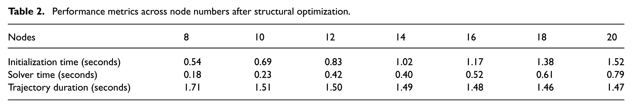
The simulation results indicate that both the computation time and the trajectory duration vary with the number of discretization nodes, as summarized in Table 2. When the number of nodes is set to 16, a favorable trade-off between motion time and computation time is achieved, and the resulting trajectory is relatively smooth.
Performance metrics across node numbers after structural optimization.
Based on the constraint ratio curves shown in Figure 6(a) and (b), the dynamic performance of the optimized trajectory is evaluated. The velocity constraint ratio and jerk constraint ratio are defined respectively as
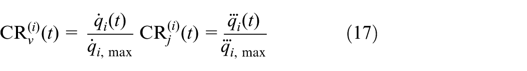
where
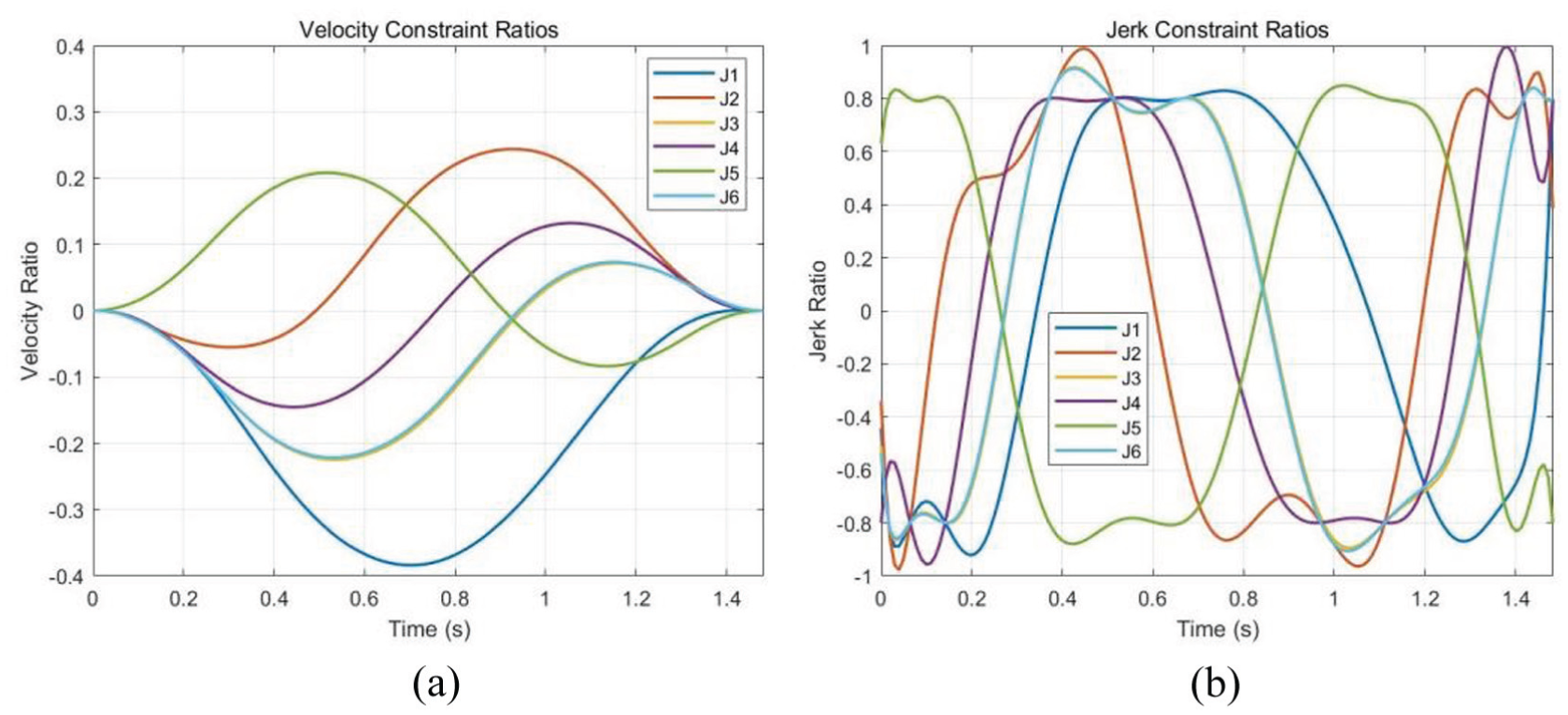
Constraint ratios of joint velocity and jerk for the robot. (a) Velocity constraint ratios. (b) Jerk constraint ratios.
A detailed analysis is conducted for the case with 16 discretization nodes to evaluate joint-level dynamic performance. As illustrated in Figure 6(a), the maximum velocity constraint ratios for all joints remain within ±0.25, significantly below the ±1 constraint boundary. This implies a minimum margin of 0.75 to the velocity limits for all joints. This indicates ample velocity margin, with smooth and continuous velocity profiles free from abrupt changes or oscillations. All joints reach their peak velocities synchronously near the midpoint of the trajectory, followed by a gradual decay, demonstrating excellent coordination and controllability of the motion.
As shown in Figure 6(b), the jerk constraint ratios approach but do not exceed the ±1 boundary in some time intervals. This suggests that the third-order dynamic response of the manipulator is actively utilized without violating physical constraints. The jerk profiles remain smooth across all joints, free from high-frequency oscillations or discontinuities, confirming the feasibility and robustness of the planned trajectory in the jerk domain.
Overall, the optimized results achieve high trajectory smoothness while keeping the computational time minimal, confirming both the efficiency and practicality of the proposed algorithm. In addition, the total trajectory duration is significantly reduced, highlighting the method’s high planning performance.
In addition, the optimization process exhibited stable numerical convergence. The IPOPT solver converged to an optimal solution after 69 iterations, with a final constraint violation of
Comparative analysis with industrial and optimization-based methods
To comprehensively evaluate the performance of the proposed framework, two representative baseline approaches are selected for comparison, namely a traditional industrial planning pipeline based on path–velocity decomposition (Rapidly-Exploring Random Trees (RRT)–Artificial Potential Fields (APF)–polynomial) and a widely adopted optimization-based trajectory planning method (CHOMP).
The first method reflects conventional industrial practice, where a collision-free geometric path is generated using RRT, smoothed by APF, and subsequently time-parameterized via polynomial interpolation. Although intuitive and computationally efficient, this approach decouples geometric planning from dynamic feasibility and therefore lacks a unified optimality formulation. CHOMP, in contrast, formulates trajectory planning as a functional optimization problem and improves smoothness through gradient-based updates. However, it primarily operates in configuration space and does not explicitly incorporate full rigid-body dynamics or time-optimal objectives.
All three methods are evaluated under identical robot models, initial and target configurations, and obstacle environments. The velocity and jerk profiles of all six joints are extracted and plotted for each trajectory, as shown in Figure 7.
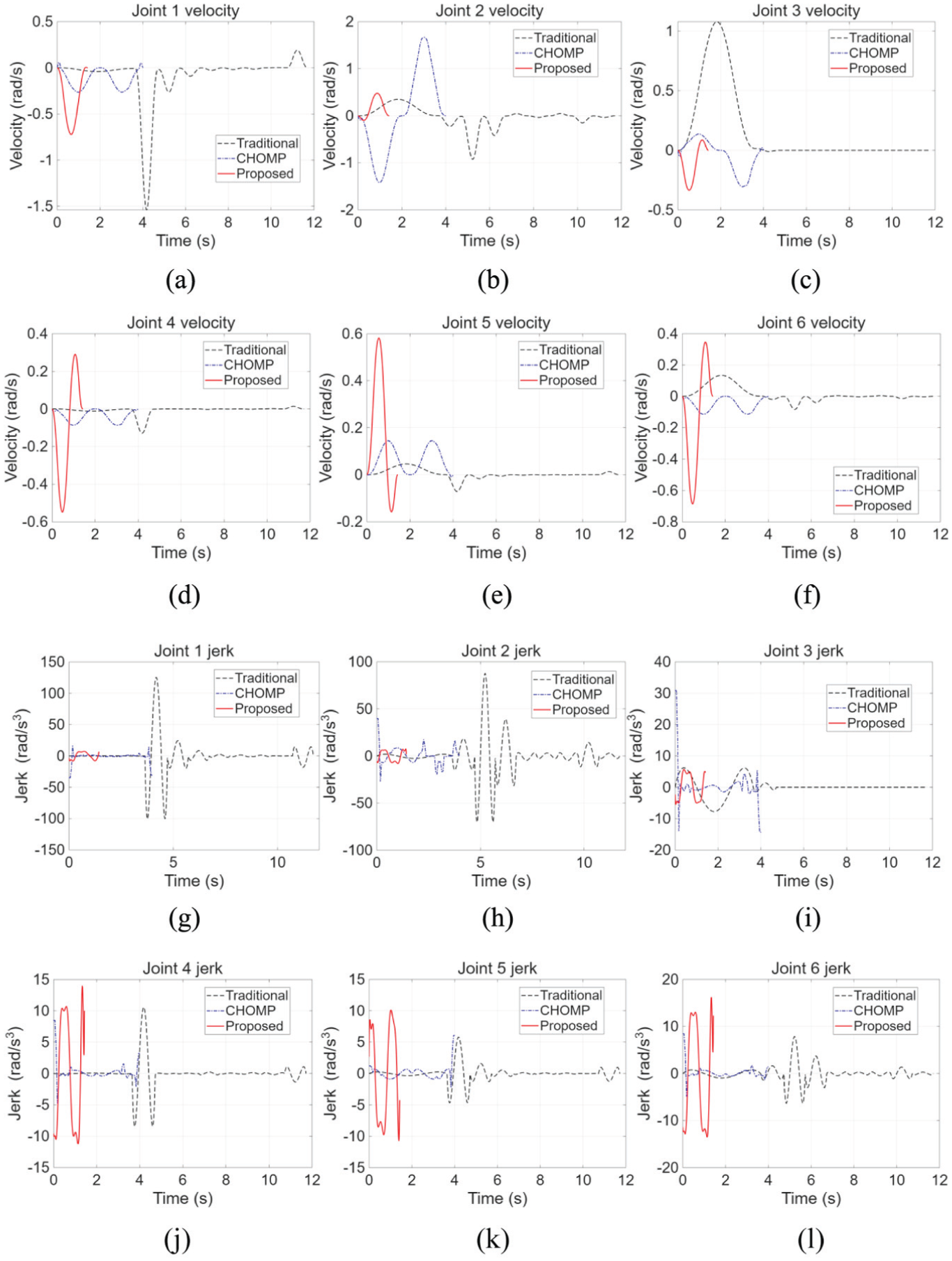
Comparison of joint velocity and jerk profiles among the traditional (RRT–APF–polynomial), CHOMP, and proposed methods. (a)–(f) Joint 1–6 velocity (rad/s). (g)–(l) Joint 1–6 jerk (rad/s3).
From the velocity curves in Figure 7(a) to (f), the traditional method exhibits significant speed fluctuations, particularly in Joints 1–3. As shown in Figure 7(a), Joint 1 displays a sharp velocity spike reaching approximately −1.5 rad/s near t = 4 seconds, followed by sustained oscillations throughout the remaining trajectory. In Figure 7(b), Joint 2 shows repeated fluctuations spanning from approximately −1.0 to 0.4 rad/s. Figure 7(c) reveals that Joint 3 reaches a peak velocity of approximately 1.1 rad/s near t = 2 seconds. In contrast, Joints 4–6 of the traditional method exhibit relatively small velocity amplitudes, as shown in Figure 7(d) to (f), with peak values below 0.15 rad/s, suggesting relatively limited participation of these joints in the overall motion under the path–velocity decomposition strategy. The overall trajectory extends over 11.72 seconds with poor inter-joint coordination.
The CHOMP method also exhibits noticeable oscillatory behavior. As shown in Figure 7(b), Joint 2 displays pronounced nonlinear fluctuations during the acceleration and deceleration phases, with the peak velocity reaching approximately 1.7 rad/s. The joint velocities require a relatively longer settling period, suggesting that the multi-joint coordination and implicit time allocation in CHOMP are not fully optimized under the given constraints.
In contrast, the velocity curves generated by the proposed method are smoother and more coordinated across all six joints. The motion task is completed within approximately 1.48 seconds, and Joints 4–6 exhibit larger velocity amplitudes than those in the traditional method, indicating more pronounced participation in the coordinated time-optimal motion. For Joints 1–3, the peak velocities are effectively constrained within the range of approximately −0.7 to 0.6 rad/s, corresponding to reductions of approximately 55% and 56% compared with the traditional method and CHOMP, respectively. It is noted that Joints 4–6 exhibit higher velocity amplitudes in the proposed method compared with the traditional approach; this is a direct consequence of the significantly shorter trajectory duration, which requires all joints to contribute more actively to complete the motion task in a time-optimal manner.
As shown in Figure 7(g) to (l), the traditional method results in several extreme jerk peaks concentrated in Joints 1 and 2. In Figure 7(g), Joint 1 reaches up to 126 rad/s3 near t = 4 seconds, while Figure 7(h) shows that Joint 2 displays abrupt, pulse-like discontinuities with magnitudes approaching 88 rad/s3. Joints 3–6 exhibit more moderate but still noticeable jerk spikes in the range of 6–11 rad/s3, as shown in Figure 7(i) to (l).
The jerk profiles of the CHOMP-based trajectory also exhibit pronounced high-frequency variations. As illustrated in Figure 7(h), Joint 2 displays sharp peaks at the beginning of the motion with magnitudes of approximately 40 rad/s3. In Figure 7(i), Joint 3 exhibits an initial jerk spike of approximately 31 rad/s3. The maximum jerk across all joints reaches approximately 40 rad/s3.
By comparison, the proposed method constrains all joint jerk values within approximately ±20 rad/s3, with continuous and smooth evolution throughout the motion. No abrupt discontinuities are observed across any of the six joints, indicating improved trajectory smoothness and dynamic consistency. The proposed method achieves an approximately 87% reduction in peak jerk compared with the traditional method and a 60% reduction compared with CHOMP.
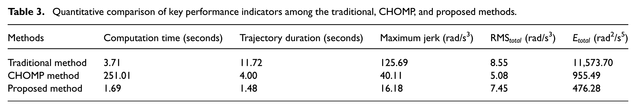
To further quantify the performance of the proposed method, Table 3 presents a detailed comparison of key performance indicators among the three approaches.
Quantitative comparison of key performance indicators among the traditional, CHOMP, and proposed methods.
Among the evaluated metrics, the overall root mean square (RMS) jerk, denoted as
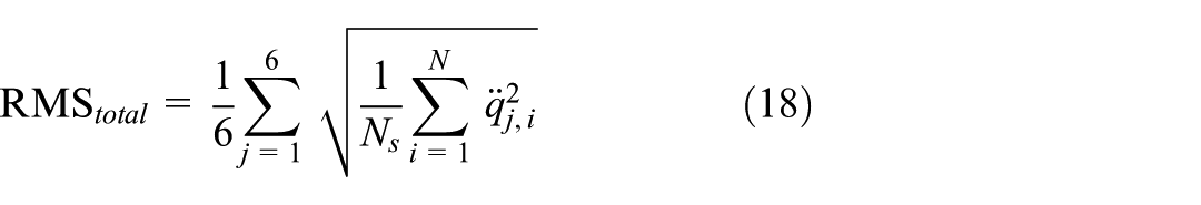
where
To incorporate the temporal resolution, the jerk energy is computed as:
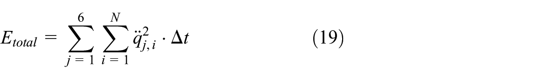
where
From the perspective of time efficiency, the proposed optimal control-based method shows clear improvements over both the traditional RRT–APF–polynomial baseline and the CHOMP method in terms of computation time and trajectory duration.
Compared with the traditional pipeline, the computation time is reduced from 3.71 seconds to 1.69 seconds (approximately 54.4%), while the overall trajectory duration decreases from 11.72 seconds to 1.48 seconds, corresponding to an 87.4% reduction in motion time.
In comparison with CHOMP, although the trajectory duration is shortened from 4.00 seconds to 1.48 seconds (a reduction of approximately 63.0%), a more pronounced difference is observed in computational cost. The CHOMP method requires 251.01 seconds to converge, whereas the proposed method completes optimization in 1.69 seconds, representing a substantial improvement in computational efficiency.
In terms of jerk-related smoothness metrics, the proposed method achieves lower maximum jerk and
For the CHOMP method, the maximum jerk reaches 40.11 rad/s3. The overall
Compared with the traditional method, the proposed approach reduces peak jerk by 87.1%, lowers
Overall, the proposed optimal control–based trajectory optimization framework achieves a favorable balance among computational efficiency, trajectory smoothness, and dynamic feasibility. The results indicate substantial reductions in motion time and jerk energy relative to the traditional method, while also offering markedly improved computational efficiency and time-optimal performance compared with CHOMP. These findings highlight the robustness and applicability of the proposed framework for complex robotic filament winding tasks.
Conclusions
This study presents a unified optimal control framework for obstacle-avoiding trajectory planning in robotic filament winding applications involving square composite tubes. The proposed formulation integrates robot dynamics, joint constraints, collision-avoidance requirements, and time-optimal objectives into a unified optimization framework based on pseudospectral transcription and AD, thereby enabling dynamically consistent trajectory generation under constrained winding environments.
Comparative simulation studies conducted on a 6-DOF industrial robot demonstrate the effectiveness of the proposed approach. Relative to the traditional RRT–APF–polynomial pipeline, the proposed method substantially reduces both computation time and trajectory duration while significantly suppressing jerk-related metrics, achieving up to 87% reduction in motion time and 96% reduction in jerk energy.
When compared with the optimization-based CHOMP method, the proposed framework exhibits markedly improved computational efficiency and shorter trajectory duration, while maintaining lower peak jerk and total jerk energy. Although CHOMP produces relatively smooth trajectories, its computational cost is considerably higher under the tested conditions. The results indicate that the proposed optimal control formulation achieves a balanced trade-off among time efficiency, smoothness, and dynamic feasibility.
Future work will focus on experimental validation through deployment on a physical robotic filament winding platform, including integration with an industrial manipulator and customized square-tube fixtures. Extensions toward real-time implementation and multi-robot coordination for advanced composite manufacturing scenarios will also be investigated.
Overall, the proposed framework provides a systematic and scalable solution for dynamically feasible and time-efficient trajectory planning in constrained filament winding environments.
Footnotes
Funding
The authors disclosed receipt of the following financial support for the research, authorship, and/or publication of this article: This work was supported by the Intelligent Filament Winding Platform for Advanced Composite Materials, Beijing University of Chemical Technology (grant number G202206230015).
Declaration of conflicting interests
The authors declared no potential conflicts of interest with respect to the research, authorship, and/or publication of this article.
Data availability statement
Data sharing is not applicable to this article, as no data sets were generated or analyzed during the current study.