Boundary feedback stabilization of a linearized compressible adiabatic flow through a porous media by backstepping method

Abstract

This paper investigates the boundary feedback stabilization of the one-dimensional linearized hyperbolic system (LHS), which models compressible adiabatic flow through porous media. The backstepping method was applied to control the LHS through Dirichlet boundary control. In this context, we proved that the solution of the LHS is exponentially stable under the effect of a designed Dirichlet feedback control law. Furthermore, the exponential decay rate depends solely on the parameters of the LHS. Finally, some numerical experiments were presented to illustrate the theoretical result.

Keywords

compressible adiabatic flow model feedback control stabilization exponential stability backstepping approach

Introduction

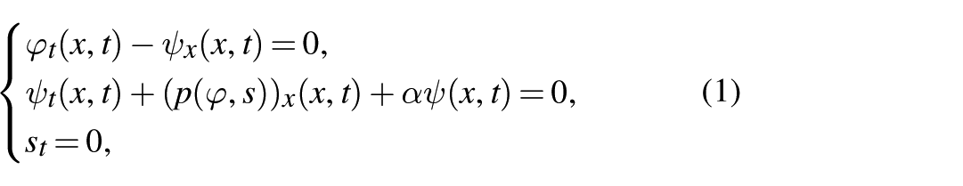
The adiabatic gas flow through a porous media is governed by the following damped hyperbolic system Maracati and Pan (2001) of first-order

\begin{matrix} {\begin{matrix} φ_{t} (x, t) - ψ_{x} (x, t) = 0, \\ ψ_{t} (x, t) + {(p (φ, s))}_{x} (x, t) + αψ (x, t) = 0, \\ s_{t} = 0, \end{matrix} \end{matrix}

(1)

where $ψ (x, t)$ is the velocity of the flow, and $φ (x, t)$ is the specific volume at a point $(x, t)$ in $ℝ \times (0, \infty)$ . Here, s is the entropy, α is a strictly positive constant, and $p > 0$ is the pressure of the gas: ${(p (φ, s))}_{φ} < 0$ , for $φ > 0$ . Assume that the pressure p satisfies the following law

\begin{matrix} p (φ, s) = (σ - 1) φ^{- σ} g^{s}, for σ > 1, \end{matrix}

(2)

where $g = g (φ, s)$ is the specific internal energy such that $p + g_{φ} = 0$ , $g_{s} \neq 0$ (this is due to the second law of thermodynamics).

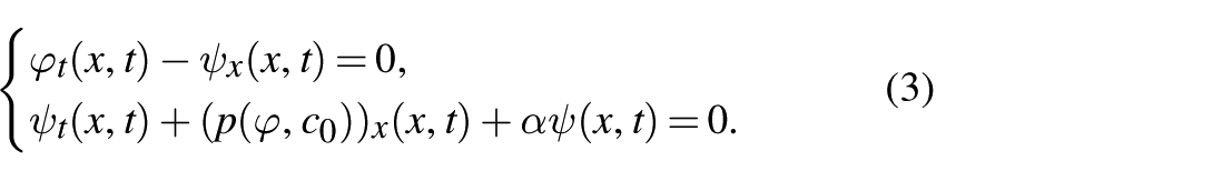
For an isentropic flow, ( $s = c_{0}$ is a constant), we rewrite the system (1) in the following form

\begin{matrix} {\begin{matrix} φ_{t} (x, t) - ψ_{x} (x, t) = 0, \\ ψ_{t} (x, t) + {(p (φ, c_{0}))}_{x} (x, t) + αψ (x, t) = 0 . \end{matrix} \end{matrix}

(3)

The initial conditions are

\begin{matrix} φ (x, 0) = φ_{0} (x), ψ (x, 0) = ψ_{0} (x), x \in ℝ . \end{matrix}

(4)

The boundary conditions are given by

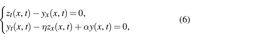
\begin{matrix} ψ (- \infty, t) = q_{-} (t), ψ (+ \infty, t) = q_{+} (t), t > 0 . \end{matrix}

(5)

Let $φ_{c}$ be a strictly positive constant. The linearized compressible adiabatic flow system around the state $(φ_{c}, 0)$ is given as follows

\begin{matrix} {\begin{matrix} z_{t} (x, t) - y_{x} (x, t) = 0, \\ y_{t} (x, t) - η z_{x} (x, t) + αy (x, t) = 0, \end{matrix} \end{matrix}

(6)

where the constant η is given by

η = g^{c_{0}} σ (σ - 1) φ_{c}^{- (σ + 1)}, σ > 1 .

For the simplicity of the analysis, we consider a bounded spatial domain $Ω = (a, b), a, b \in ℝ$ , ( $a < b$ ). In this case, we have the following initial conditions

\begin{matrix} z (x, 0) = z_{0} (x), y (x, 0) = y_{0} (x), x \in Ω . \end{matrix}

(7)

The boundary conditions are given by

\begin{matrix} y (a, t) = q_{a} (t), y (b, t) = q_{b} (t), t > 0 . \end{matrix}

(8)

Definition 1. The systems (6)–(8) are said to be exponentially stable in a Hilbert space $Z$ , if there exists a strictly positive constant ν such that

\begin{matrix} ∥ (z, y) (t) ∥_{Z} \leq M e^{- νt} ∥ (z_{0}, y_{0}) ∥_{Z}, \forall t \geq 0, \end{matrix}

(9)

where M is a positive constant.

Consider one Dirichlet boundary condition, for example, on the right side $x = b$ , that is,

\begin{matrix} y (a, t) = 0, y (b, t) = q_{b} (t), t > 0 . \end{matrix}

(10)

To stabilize the systems (6)–(7) and (10), in the sense of Definition 1, we look for a boundary control $q_{b} \in H$ in feedback form such that

\begin{matrix} q_{b} (t) = K (z (\cdot, t), y (\cdot, t)), t \geq 0, \end{matrix}

(11)

where $K$ is a continuous linear bounded operator defined from $Z$ into $H$ .

Stabilization of nonlinear hyperbolic systems of first/second order has interested many researchers, such as Aamo (2006), Castillo et al. (2013a), Castillo et al. (2013b), and Krstic and Smyshlyaev (2008). In Coron et al. (2021), the authors studied the boundary stabilization in finite time of the one-dimensional linear hyperbolic balance laws with coefficients depending on time and space by the backstepping approach. In Amaury (2021), the author studied and presented various methods and techniques for the stabilization of nonlinear hyperbolic systems using boundary controls but without using the backstepping approach. In Castillo et al. (2016), a polytopic method is developed for quasilinear hyperbolic systems in order to guarantee stability in a given region around an equilibrium point.

In Maddouri (2024), the exponential stability of the linearized hyperbolic system (LHS) (6) and (7) with homogeneous Dirichlet boundary conditions ( $q_{a} = q_{b} \equiv 0$ ) has been investigated. This result was obtained through an in-depth analysis of the spectrum of the linear operator associated with the systems (6)–(7). Using explicit calculations, the author proved that the solution decreases exponentially with a decay rate equal to $ν = \frac{α}{2}$ . In fact, the rate $ν = \frac{α}{2}$ represents an accumulation point of the eigenvalues of the associated linear operator (for more details, we refer readers to Maddouri (2024)). The question that now arises: is it possible to have exponential stability of the systems (6)–(7), with nonzero Dirichlet conditions? The answer is no, because, in general, the solution is unstable in this case, except with an appropriate choice of Dirichlet boundary conditions.

In this paper, we study Dirichlet boundary feedback stabilization for the unstable LHS (6)–(7)+(10). In fact, the backstepping method was applied to construct a Dirichlet boundary feedback control law which allows for obtaining exponential stability for the original LHS (6)–(7)+(10). The backtracking method is an approach that consists of transforming the original LHS (6)–(7)+(10) into a target hyperbolic system for which stability is simpler to study. To obtain the desired transformation, we have applied the Volterra transformations of the second kind (Coron et al., 2021), which are invertible, continuous, and bounded.

The stabilization of one-dimensional boundary systems and the use of Volterra transformations of the second kind correspond together. Since Volterra transformations eliminate in a certain way the unwanted terms (or add supporting terms), which influence the stabilization of the system by expelling them to the boundary part where the feedback law is acting. This method has rapidly demonstrated its great capability to be very successful in the analysis and study of the boundary stabilization of several and various problems governed by PDEs such as Schrödinger equations, reaction–diffusion equations (Zhou and Guo, 2018), heat equations (Liu, 2022), and Navier–Stokes systems (Chowdhury et al., 2021).

It is well known that hyperbolic systems of first order are much less stable than parabolic systems. In fact, for one-dimensional parabolic systems, second derivative terms of the form ( $μ \partial_{xx}$ , $μ > 0$ ) play a motivating role for a rapid stabilization of solutions, unlike hyperbolic systems of the first order. Therefore, the stabilization of first-order hyperbolic systems represents a major challenge in this work. Our goal is therefore to build a robust Dirichlet-type boundary feedback control law, allowing us to overcome undesirable instabilities and achieve rapid stabilization.

The content of this paper is organized as follows. First, the exponential stability and the regularity of the global solution of the target LHS have been investigated (Theorems 3 and 4). Then, using the backstepping method, we have designed the feedback controller (45). The main result of this paper is given in Theorem 5. The final section of this paper has been reserved for the numerical implementation of the closed-loop system (47) and the interpretation of the numerical results.

Target hyperbolic system

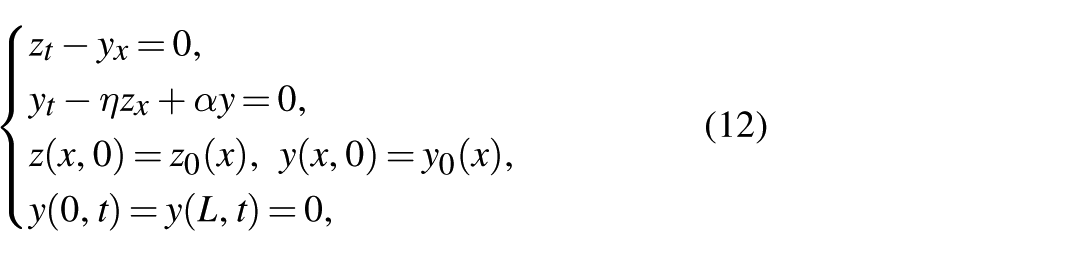
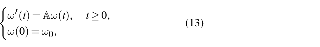
Let $Ω = (0, L)$ , $L > 0$ . Let us introduce the following target system with homogeneous Dirichlet boundary conditions

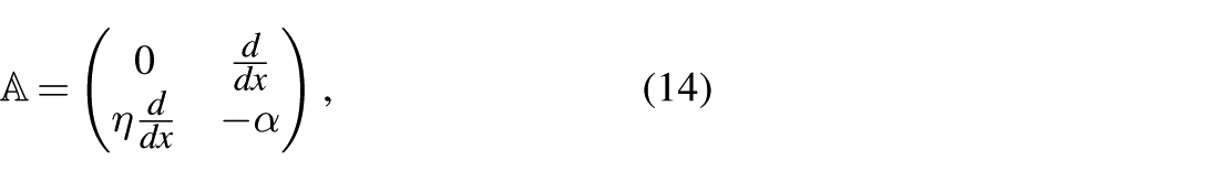
\begin{matrix} {\begin{matrix} z_{t} - y_{x} = 0, \\ y_{t} - η z_{x} + αy = 0, \\ z (x, 0) = z_{0} (x), y (x, 0) = y_{0} (x), \\ y (0, t) = y (L, t) = 0, \end{matrix} \end{matrix}

(12)

for all $(x, t) \in Ω \times (0, \infty)$ , where $η, α$ are the two strictly positive real numbers. Let $ω (t) = (z (\cdot, t), y (\cdot, t))$ , and $ω_{0} = (z_{0} (\cdot), y_{0} (\cdot))$ . Then, we rewrite the system (12) as follows

\begin{matrix} {\begin{matrix} ω^{'} (t) = A ω (t), t \geq 0, \\ ω (0) = ω_{0}, \end{matrix} \end{matrix}

(13)

where $ω^{'} (t) = \frac{dω (t)}{dt}$ and the differential operator $A$ is given by

\begin{matrix} A = (\begin{matrix} 0 & \frac{d}{dx} \\ η \frac{d}{dx} & - α \end{matrix}), \end{matrix}

(14)

with domain $D (A)$ given by

\begin{matrix} D (A) = H^{1} (Ω) \times H_{0}^{1} (Ω) . \end{matrix}

(15)

In Maddouri (2024), it was proven that $(A, D (A))$ is the infinitesimal generator of a strongly continuous semigroup of contractions on $L^{2} (Ω) = L^{2} (Ω) \times L^{2} (Ω)$ denoted by $S (t) = e^{- t A}, t \geq 0$ . In Maddouri (2024), recall that the space $L^{2} (Ω)$ is equipped with the scalar product ${(v, u)}_{L^{2} (Ω)} = η \int_{Ω} v_{1} u_{1} + \int_{Ω} v_{2} u_{2}$ for all $v = (v_{1}, v_{2})$ and $u = (u_{1}, u_{2})$ . Therefore, the following theorem holds.

Theorem 1. (Maddouri, 2024) For any $ω_{0} \in L^{2} (Ω)$ , the target system (13) has a unique solution $ω \in C ([0, \infty); L^{2} (Ω))$ such that

\begin{matrix} ∥ ω (t) ∥_{L^{2} (Ω)} \leq ∥ ω_{0} ∥_{L^{2} (Ω)}, \forall t \geq 0 . \end{matrix}

(16)

Furthermore, we have the following theorem.

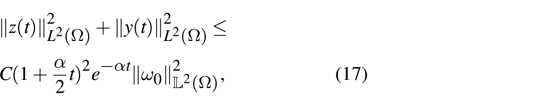
Theorem 2. (Maddouri, 2024). For all $ω_{0} \in L^{2} (Ω)$ , there exists $C > 0$ such that the solution $ω = (z, y)$ to the target system (13) satisfies the estimate

\begin{matrix} ∥ z (t) ∥_{L^{2} (Ω)}^{2} + ∥ y (t) ∥_{L^{2} (Ω)}^{2} \leq \\ C {(1 + \frac{α}{2} t)}^{2} e^{- αt} ∥ ω_{0} ∥_{L^{2} (Ω)}^{2}, \end{matrix}

(17)

for all $t \geq 0$ , where α is given in the system (12).

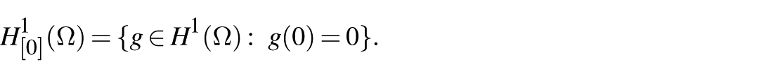
Let $ℍ^{1} (Ω)$ be the Hilbert space defined by $ℍ^{1} (Ω) = H^{1} (Ω) \times H_{0}^{1} (Ω)$ . In Maddouri (2024), the space $ℍ^{1} (Ω)$ is equipped with the scalar product ${(v, u)}_{ℍ^{1} (Ω)} = η \int_{Ω} v_{1}^{'} u_{1}^{'} + \int_{Ω} v_{2}^{'} u_{2}^{'}$ , for all $v = (v_{1}, v_{2})$ and $u = (u_{1}, u_{2})$ . Due to the Poincaré–Wirtinger and Poincaré inequalities, the associated norm $∥ \cdot ∥_{ℍ^{1} (Ω)}$ is equivalent to the usual norm of $H^{1} (Ω) \times H_{0}^{1} (Ω)$ .

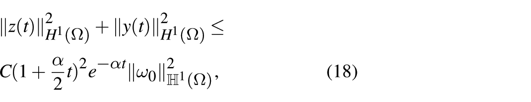
Theorem 3. (Maddouri, 2024). For all $ω_{0} \in ℍ^{1} (Ω)$ , there exists $C > 0$ such that the solution $ω = (z, y)$ to the target system (13) satisfies the estimate

\begin{matrix} ∥ z (t) ∥_{H^{1} (Ω)}^{2} + ∥ y (t) ∥_{H^{1} (Ω)}^{2} \leq \\ C {(1 + \frac{α}{2} t)}^{2} e^{- αt} ∥ ω_{0} ∥_{ℍ^{1} (Ω)}^{2}, \end{matrix}

(18)

for all $t \geq 0$ , where α is given in the system (12).

The regularity of the solution to the system (12) is provided in the following theorem.

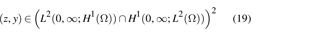
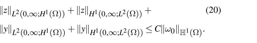
Theorem 4. For all $ω_{0} \in ℍ^{1} (Ω)$ , there exists $C > 0$ such that the solution $ω = (z, y)$ of the target system (13) is

\begin{matrix} (z, y) \in (L^{2} (0, \infty; H^{1} (Ω)) \cap H^{1} (0, \infty; L^{2} (Ω)))^{2} \end{matrix}

(19)

and satisfies the estimate

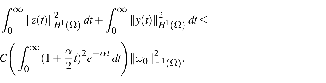
\begin{matrix} ∥ z ∥_{L^{2} (0, \infty; H^{1} (Ω))} + ∥ z ∥_{H^{1} (0, \infty; L^{2} (Ω))} + \\ ∥ y ∥_{L^{2} (0, \infty; H^{1} (Ω))} + ∥ y ∥_{H^{1} (0, \infty; L^{2} (Ω))} \leq C ∥ ω_{0} ∥_{ℍ^{1} (Ω)} . \end{matrix}

(20)

Proof. From (18) and by integration with respect to t on $[0, \infty)$ , we get

\begin{matrix} \int_{0}^{\infty} ∥ z (t) ∥_{H^{1} (Ω)}^{2} dt + \int_{0}^{\infty} ∥ y (t) ∥_{H^{1} (Ω)}^{2} dt \leq \\ C (\int_{0}^{\infty} {(1 + \frac{α}{2} t)}^{2} e^{- αt} dt) ∥ ω_{0} ∥_{ℍ^{1} (Ω)}^{2} . \end{matrix}

Then, with simple calculation, we obtain the following

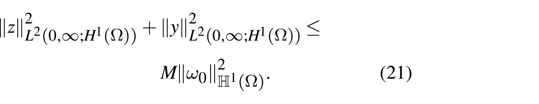
\begin{matrix} ∥ z ∥_{L^{2} (0, \infty; H^{1} (Ω))}^{2} & + ∥ y ∥_{L^{2} (0, \infty; H^{1} (Ω))}^{2} \leq \\ M ∥ ω_{0} ∥_{ℍ^{1} (Ω)}^{2} . \end{matrix}

(21)

where the constant $M > 0$ . Then, we deduce that

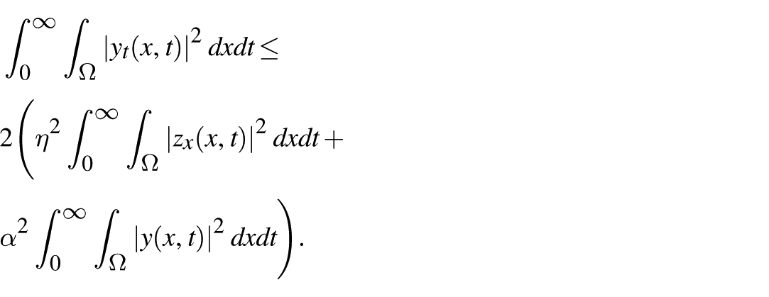
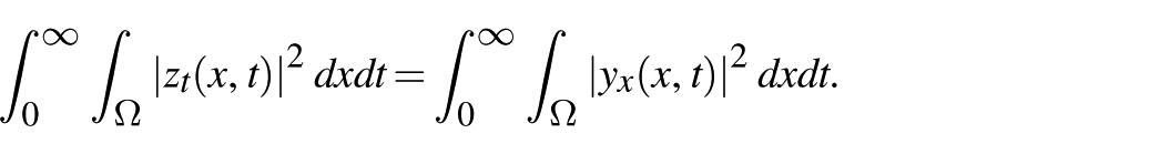
(z, y) \in L^{2} (0, \infty; H^{1} (Ω)) \times L^{2} (0, \infty; H^{1} (Ω)) .

Now, from the second equation of the system (12) and by integration with respect to x and t on $Ω \times (0, \infty)$ , we obtain

\begin{matrix} \int_{0}^{\infty} \int_{Ω} | y_{t} (x, t) |^{2} dxdt \leq \\ 2 (η^{2} \int_{0}^{\infty} \int_{Ω} | z_{x} (x, t) |^{2} dxdt + \\ α^{2} \int_{0}^{\infty} \int_{Ω} | y (x, t) |^{2} dxdt) . \end{matrix}

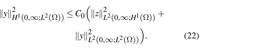
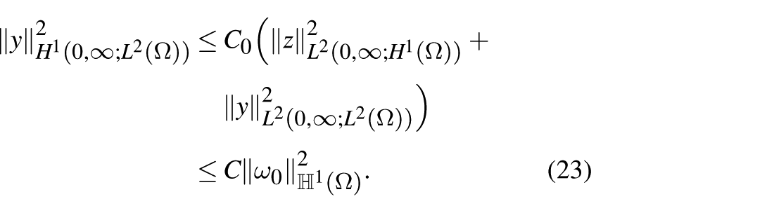
It follows that

\begin{matrix} ∥ y ∥_{H^{1} (0, \infty; L^{2} (Ω))}^{2} \leq & C_{0} (∥ z ∥_{L^{2} (0, \infty; H^{1} (Ω))}^{2} + \\ ∥ y ∥_{L^{2} (0, \infty; L^{2} (Ω))}^{2}) . \end{matrix}

(22)

Using (21) and (22), we get

\begin{matrix} ∥ y ∥_{H^{1} (0, \infty; L^{2} (Ω))}^{2} \leq & C_{0} (∥ z ∥_{L^{2} (0, \infty; H^{1} (Ω))}^{2} + \\ ∥ y ∥_{L^{2} (0, \infty; L^{2} (Ω))}^{2}) \\ \leq C ∥ ω_{0} ∥_{ℍ^{1} (Ω)}^{2} . \end{matrix}

(23)

which implies that $y \in H^{1} (0, \infty; L^{2} (Ω))$ . From the first equation of system (12), we get

\begin{matrix} \int_{0}^{\infty} \int_{Ω} | z_{t} (x, t) |^{2} dxdt = \int_{0}^{\infty} \int_{Ω} | y_{x} (x, t) |^{2} dxdt . \end{matrix}

Then, we deduce that

\begin{matrix} ∥ z ∥_{H^{1} (0, \infty; L^{2} (Ω))}^{2} \leq & ∥ y ∥_{L^{2} (0, \infty; H^{1} (Ω))}^{2} + \\ ∥ z ∥_{L^{2} (0, \infty; L^{2} (Ω))}^{2} . \end{matrix}

(24)

Now, from (21) and (24), it follows that

\begin{matrix} ∥ z ∥_{H^{1} (0, \infty; L^{2} (Ω))}^{2} \leq M ∥ ω_{0} ∥_{ℍ^{1} (Ω)}^{2} . \end{matrix}

(25)

Therefore, $z \in H^{1} (0, \infty; L^{2} (Ω))$ . The estimate (20) can be obtained from relations (21), (23), and (25). The proof is completed.

Backstepping transform and feedback control law

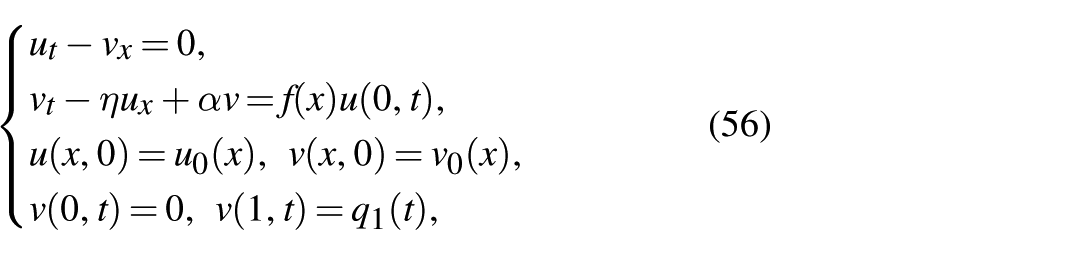
Let $Ω = (0, L)$ , $L > 0$ . We are interested in the LHS with non-homogeneous boundary conditions. We study the stabilization of the LHS by only one control on the right-hand side of the interval $Ω$ ; thus, we have

\begin{matrix} {\begin{matrix} u_{t} - v_{x} = 0, \\ v_{t} - η u_{x} + αv = f (x) u (0, t), \\ u (x, 0) = u_{0} (x), v (x, 0) = v_{0} (x), \\ v (0, t) = 0, v (L, t) = q_{L} (t), \end{matrix} \end{matrix}

(26)

for all $(x, t) \in Ω \times (0, \infty)$ , where f is a continuous function on the interval $[0, L]$ such that $f (0) \neq 0$ .

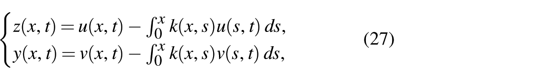
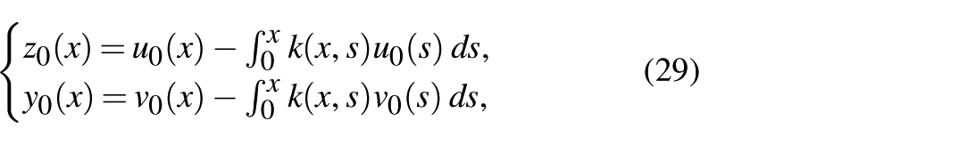
To construct the Dirichlet boundary control $q_{L} (t)$ for the stabilization of the system (26), we introduce the following integral transformations

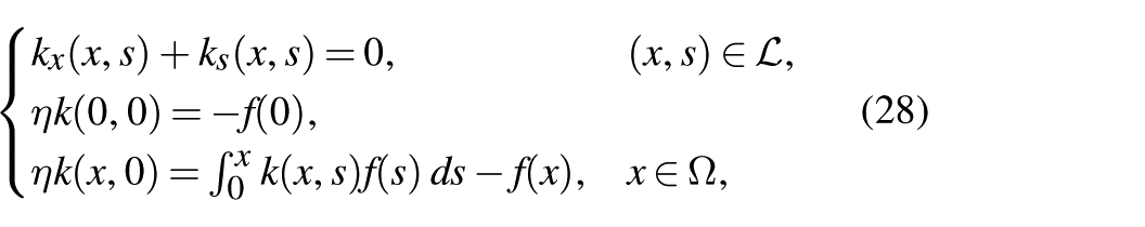
\begin{matrix} {\begin{matrix} z (x, t) = u (x, t) - \int_{0}^{x} k (x, s) u (s, t) ds, \\ y (x, t) = v (x, t) - \int_{0}^{x} k (x, s) v (s, t) ds, \end{matrix} \end{matrix}

(27)

where the kernel function k verifies the following system

\begin{matrix} {\begin{matrix} k_{x} (x, s) + k_{s} (x, s) = 0, & (x, s) \in L, \\ ηk (0, 0) = - f (0), \\ ηk (x, 0) = \int_{0}^{x} k (x, s) f (s) ds - f (x), & x \in Ω, \end{matrix} \end{matrix}

(28)

where the set $L$ is defined by

L = {(x, s) \in [0, L] \times [0, L], s \leq x} .

It can be shown that the system (28) has a unique solution $k \in C^{0} (L)$ (Coron et al., 2021, Theorem 2.6). Note that transformations (27) are invertible (Coron et al., 2021; Zhou and Guo, 2018). Then, using transformations (27), we can convert the system (26) to the target system (12) with initial conditions

\begin{matrix} {\begin{matrix} z_{0} (x) = u_{0} (x) - \int_{0}^{x} k (x, s) u_{0} (s) ds, \\ y_{0} (x) = v_{0} (x) - \int_{0}^{x} k (x, s) v_{0} (s) ds, \end{matrix} \end{matrix}

(29)

and vice versa. Moreover, stability for the system (26) can be deduced from the stability of the target systems (12), (29), and (27).

Proposition 1. Let k be the solution of the system (28). Then, the target system (12) with initial conditions (29), and under the invertible transformations (27), is equivalent to the system (26) and vice versa.

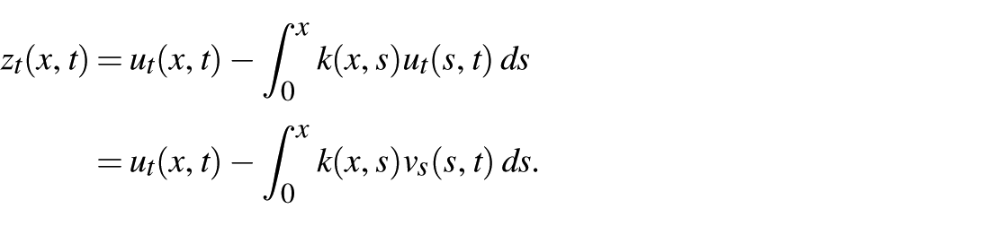
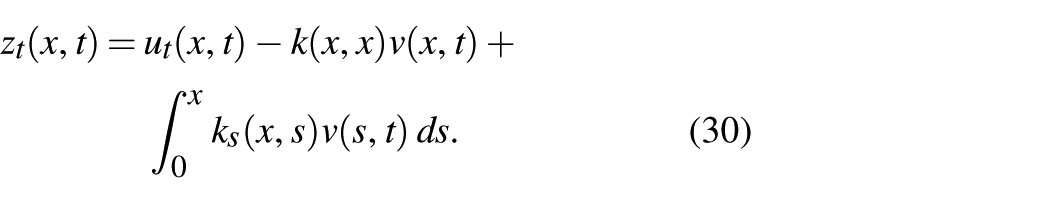
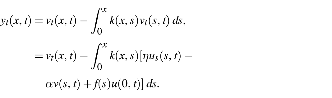
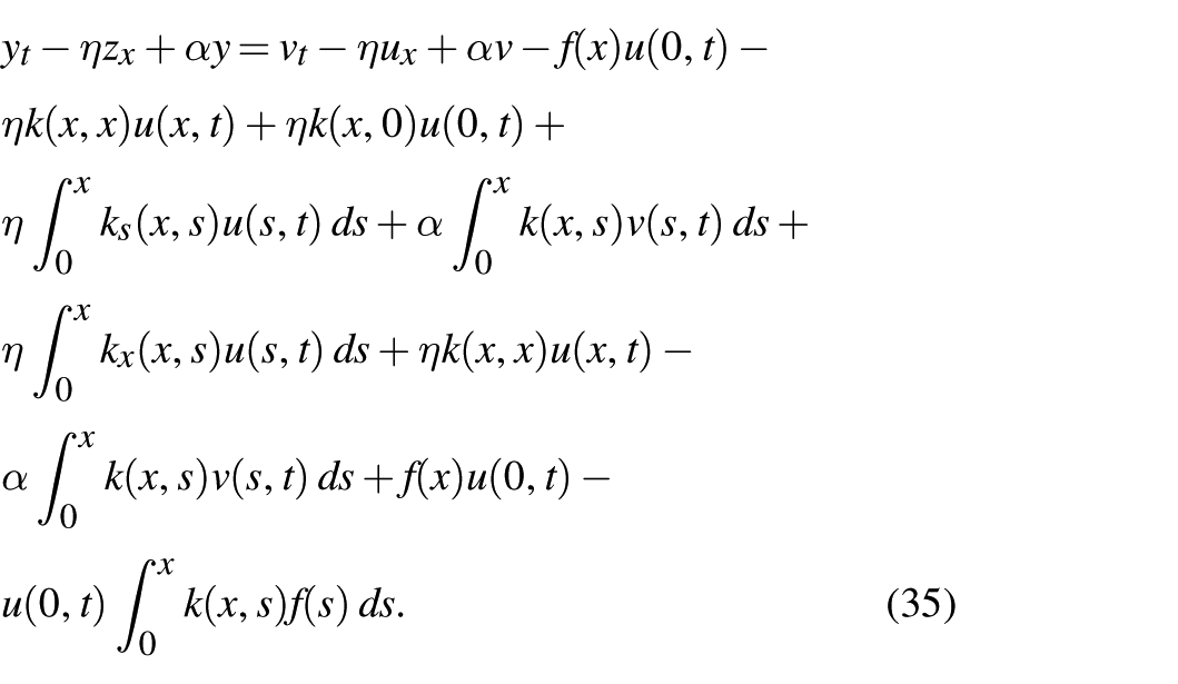
Proof. Differentiating the first equation of (27) with respect to the time t and using the first equation of (26), we get

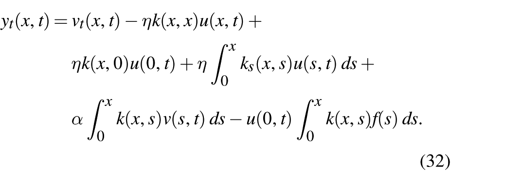
\begin{matrix} z_{t} (x, t) & = u_{t} (x, t) - \int_{0}^{x} k (x, s) u_{t} (s, t) ds \\ = u_{t} (x, t) - \int_{0}^{x} k (x, s) v_{s} (s, t) ds . \end{matrix}

Using integration by parts, we obtain

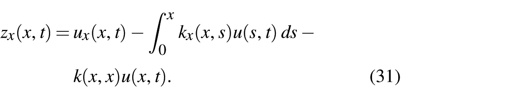
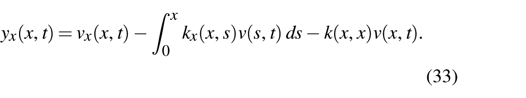
\begin{matrix} z_{t} (x, t) = & u_{t} (x, t) - k (x, x) v (x, t) + \\ \int_{0}^{x} k_{s} (x, s) v (s, t) ds . \end{matrix}

(30)

Also, by differentiating the first equation of (27) with respect to x, we obtain

\begin{matrix} z_{x} (x, t) = & u_{x} (x, t) - \int_{0}^{x} k_{x} (x, s) u (s, t) ds - \\ k (x, x) u (x, t) . \end{matrix}

(31)

Now, differentiating the second equation of (27) with respect to t and using the second equation of (26), we get

\begin{matrix} y_{t} (x, t) = & v_{t} (x, t) - \int_{0}^{x} k (x, s) v_{t} (s, t) ds, \\ = & v_{t} (x, t) - \int_{0}^{x} k (x, s) [η u_{s} (s, t) - \\ αv (s, t) + f (s) u (0, t)] ds . \end{matrix}

After integration by parts, it follows that

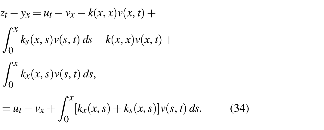
\begin{matrix} y_{t} (x, t) = & v_{t} (x, t) - ηk (x, x) u (x, t) + \\ ηk (x, 0) u (0, t) + η \int_{0}^{x} k_{s} (x, s) u (s, t) ds + \\ α \int_{0}^{x} k (x, s) v (s, t) ds - u (0, t) \int_{0}^{x} k (x, s) f (s) ds . \end{matrix}

(32)

Again, differentiating the second equation of (27) with respect to x, yields

\begin{matrix} y_{x} (x, t) = & v_{x} (x, t) - \int_{0}^{x} k_{x} (x, s) v (s, t) ds - k (x, x) v (x, t) . \end{matrix}

(33)

By combining equations (30) and (33), we obtain

\begin{matrix} z_{t} - y_{x} = u_{t} - v_{x} - k (x, x) v (x, t) + \\ \int_{0}^{x} k_{s} (x, s) v (s, t) ds + k (x, x) v (x, t) + \\ \int_{0}^{x} k_{x} (x, s) v (s, t) ds, \\ = u_{t} - v_{x} + \int_{0}^{x} [k_{x} (x, s) + k_{s} (x, s)] v (s, t) ds . \end{matrix}

(34)

Again, by combining equations (31) and (32), we get

\begin{matrix} y_{t} - η z_{x} + αy = v_{t} - η u_{x} + αv - f (x) u (0, t) - \\ ηk (x, x) u (x, t) + ηk (x, 0) u (0, t) + \\ η \int_{0}^{x} k_{s} (x, s) u (s, t) ds + α \int_{0}^{x} k (x, s) v (s, t) ds + \\ η \int_{0}^{x} k_{x} (x, s) u (s, t) ds + ηk (x, x) u (x, t) - \\ α \int_{0}^{x} k (x, s) v (s, t) ds + f (x) u (0, t) - \\ u (0, t) \int_{0}^{x} k (x, s) f (s) ds . \end{matrix}

(35)

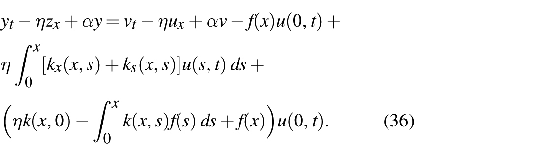
After rearranging the terms on the right-hand side of the equation (35), we obtain

\begin{matrix} y_{t} - η z_{x} + αy = v_{t} - η u_{x} + αv - f (x) u (0, t) + \\ η \int_{0}^{x} [k_{x} (x, s) + k_{s} (x, s)] u (s, t) ds + \\ (ηk (x, 0) - \int_{0}^{x} k (x, s) f (s) ds + f (x)) u (0, t) . \end{matrix}

(36)

Now, as $(u, v)$ is a solution of the system (26), and $k (x, s)$ is the solution of system (28), then we deduce from equations (34)–(36) the target system (12). Similarly, it is easy to prove the converse.

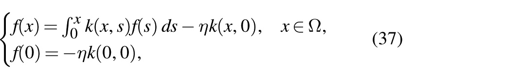
Remark 1. For a given kernel function $k (x, s)$ , the Volterra integral equation

\begin{matrix} {\begin{matrix} f (x) = \int_{0}^{x} k (x, s) f (s) ds - ηk (x, 0), & x \in Ω, \\ f (0) = - ηk (0, 0), \end{matrix} \end{matrix}

(37)

has a unique global solution $f (x)$ .

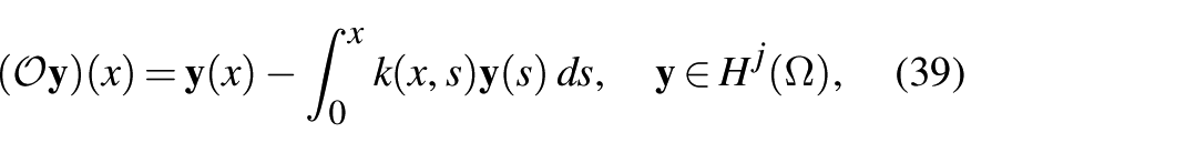
Remark 2. Let $O$ be a linear bounded operator defined by

\begin{matrix} O : H^{j} (Ω) \to H^{j} (Ω) ∕ y ⟼ O y, j = 0, 1, 2, \end{matrix}

(38)

such that

\begin{matrix} (O y) (x) = y (x) - \int_{0}^{x} k (x, s) y (s) ds, y \in H^{j} (Ω), \end{matrix}

(39)

where $k (x, s)$ is the solution of the system (28). From Liu (2022, Lemma 2.4), the linear bounded operator $O$ is continuous and has a linear bounded and continuous inverse $O^{- 1}$ defined from $H^{j} (Ω)$ into $H^{j} (Ω)$ , for $j = 0, 1, 2$ .

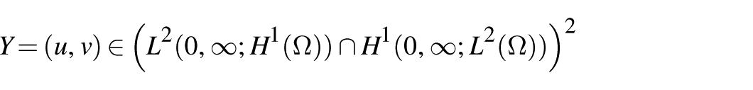
Let $H_{[0]}^{1} (Ω)$ be the space defined by

H_{[0]}^{1} (Ω) = {g \in H^{1} (Ω) : g (0) = 0} .

Proposition 2. For all $Y_{0} = (u_{0}, v_{0}) \in H^{1} (Ω) \times H_{[0]}^{1} (Ω)$ , the system (26) has a unique solution

Y = (u, v) \in (L^{2} (0, \infty; H^{1} (Ω)) \cap H^{1} (0, \infty; L^{2} (Ω)))^{2}

and satisfies the estimate

\begin{matrix} ∥ u ∥_{L^{2} (0, \infty; H^{1} (Ω))} + ∥ u ∥_{H^{1} (0, \infty; L^{2} (Ω))} + \\ ∥ v ∥_{L^{2} (0, \infty; H^{1} (Ω))} + ∥ v ∥_{H^{1} (0, \infty; L^{2} (Ω))} \leq \\ C ∥ Y_{0} ∥_{ℍ^{1} (Ω)} . \end{matrix}

(40)

Proof. Recall that $ω_{0} = (z_{0}, y_{0})$ and $ω = (z, y)$ is the solution of the target system (12). Now, using the transformations (27) and the definition of the operator $O$ given by Remark 2, we have

\begin{matrix} ω = O Y and ω_{0} = O Y_{0} \end{matrix}

(41)

where $Y_{0} = (u_{0}, v_{0})$ and $Y = (u, v)$ is the solution of the original system (26). Consequently, since the operator $O$ is invertible, we get

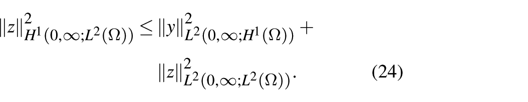
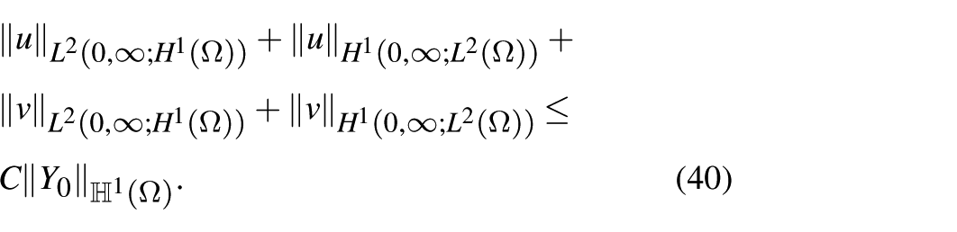
\begin{matrix} u = O^{- 1} z and v = O^{- 1} y, \end{matrix}

(42)

By substituting (42) in the term on the left side of equation (40) and using the continuity of $O^{- 1}$ and the estimate (20), we get

\begin{matrix} ∥ u ∥_{L^{2} (0, \infty; H^{1} (Ω))} + ∥ u ∥_{H^{1} (0, \infty; L^{2} (Ω))} + \\ ∥ v ∥_{H^{1} (0, \infty; L^{2} (Ω))} + ∥ v ∥_{L^{2} (0, \infty; H^{1} (Ω))} = \\ ∥ O^{- 1} z ∥_{L^{2} (0, \infty; H^{1} (Ω))} + ∥ O^{- 1} z ∥_{H^{1} (0, \infty; L^{2} (Ω))} + \\ ∥ O^{- 1} y ∥_{H^{1} (0, \infty; L^{2} (Ω))} + ∥ O^{- 1} y ∥_{L^{2} (0, \infty; H^{1} (Ω))} \leq \\ C (∥ z ∥_{L^{2} (0, \infty; H^{1} (Ω))} + ∥ z ∥_{H^{1} (0, \infty; L^{2} (Ω))} + \\ ∥ y ∥_{H^{1} (0, \infty; L^{2} (Ω))} + ∥ y ∥_{L^{2} (0, \infty; H^{1} (Ω))}) \leq \\ C ∥ ω_{0} ∥_{ℍ^{1} (Ω)} . \end{matrix}

(43)

Now, using relation (41) and the continuity of the operator $O$ , it follows that

\begin{matrix} ∥ ω_{0} ∥_{ℍ^{1} (Ω)} \leq C ∥ Y_{0} ∥_{ℍ^{1} (Ω)} . \end{matrix}

(44)

Therefore, estimates (43) and (44) lead to estimate (40) and then the regularity of $Y = (u, v)$ .

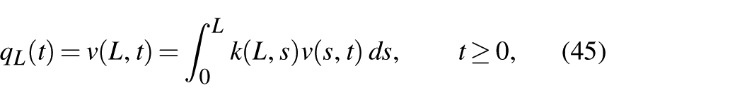
To achieve the stabilization of the system (26), the designed Dirichlet boundary control $q_{L} (t)$ is given by

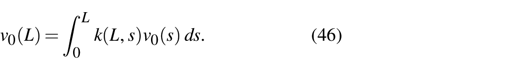
\begin{matrix} q_{L} (t) = v (L, t) = \int_{0}^{L} k (L, s) v (s, t) ds, t \geq 0, \end{matrix}

(45)

where $k (x, s)$ is the solution of system (28). Since $v \in L^{2} (0, \infty; H^{1} (Ω)) \cap H^{1} (0, \infty; L^{2} (Ω))$ , then $q_{L} \in H^{1} (0, \infty)$ . Moreover, the control $q_{L}$ and the initial condition $v_{0}$ are related by the following compatibility condition

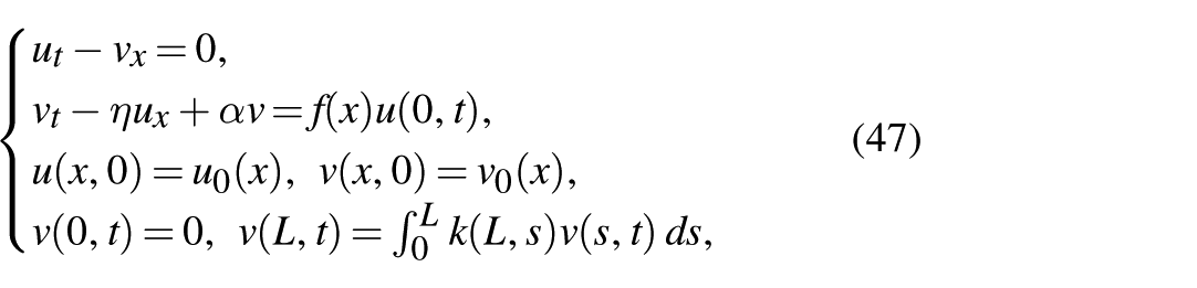
\begin{matrix} v_{0} (L) = \int_{0}^{L} k (L, s) v_{0} (s) ds . \end{matrix}

(46)

Under the designed feedback control law (45), the closed-loop of the system (26) is given by

\begin{matrix} {\begin{matrix} u_{t} - v_{x} = 0, \\ v_{t} - η u_{x} + αv = f (x) u (0, t), \\ u (x, 0) = u_{0} (x), v (x, 0) = v_{0} (x), \\ v (0, t) = 0, v (L, t) = \int_{0}^{L} k (L, s) v (s, t) ds, \end{matrix} \end{matrix}

(47)

for all $(x, t) \in Ω \times (0, \infty)$ . As previously demonstrated, the system (47) is equivalent to the target system (12).

The main result of this paper is given in the following theorem.

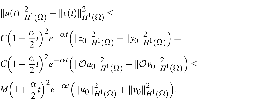
Theorem 5. For any initial condition $(u_{0}, v_{0}) \in H^{1} (Ω) \times H_{[0]}^{1} (Ω)$ such that

\begin{matrix} v_{0} (L) = \int_{0}^{L} k (L, s) v_{0} (s) ds, \end{matrix}

(48)

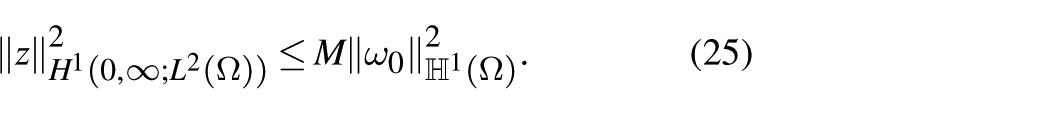
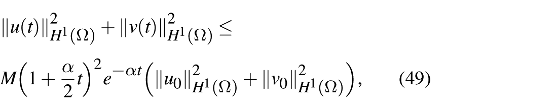
the system (47) has a unique solution $(u, v)$ that satisfies the following stability estimate

\begin{matrix} ∥ u (t) ∥_{H^{1} (Ω)}^{2} + ∥ v (t) ∥_{H^{1} (Ω)}^{2} \leq \\ M (1 + \frac{α}{2} t)^{2} e^{- αt} (∥ u_{0} ∥_{H^{1} (Ω)}^{2} + ∥ v_{0} ∥_{H^{1} (Ω)}^{2}), \end{matrix}

(49)

for all $t \geq 0$ , where M is a positive constant.

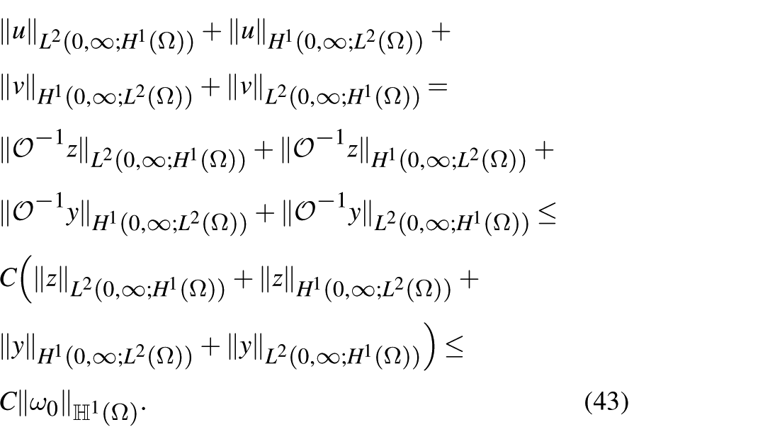
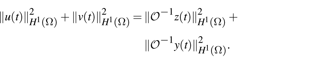
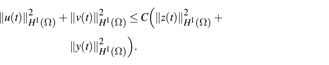
Proof. Let $(u_{0}, v_{0}) \in H^{1} (Ω) \times H_{[0]}^{1} (Ω)$ such that the compatibility condition (48) is satisfied. Then, from the transformations given in (29), the relations (41) and (42), and Remark 2 combined with the estimate (18), we can establish the estimate (49). From (42), we have

\begin{matrix} ∥ u (t) ∥_{H^{1} (Ω)}^{2} + ∥ v (t) ∥_{H^{1} (Ω)}^{2} = & ∥ O^{- 1} z (t) ∥_{H^{1} (Ω)}^{2} + \\ ∥ O^{- 1} y (t) ∥_{H^{1} (Ω)}^{2} . \end{matrix}

The operator $O^{- 1}$ is continuous, then there exists a constant C such that

\begin{matrix} ∥ u (t) ∥_{H^{1} (Ω)}^{2} + & ∥ v (t) ∥_{H^{1} (Ω)}^{2} \leq C (∥ z (t) ∥_{H^{1} (Ω)}^{2} + \\ ∥ y (t) ∥_{H^{1} (Ω)}^{2}) . \end{matrix}

By estimate (18), relation (41), and the continuity of the operator $O$ , it follows that

\begin{matrix} ∥ u (t) ∥_{H^{1} (Ω)}^{2} + ∥ v (t) ∥_{H^{1} (Ω)}^{2} \leq \\ C (1 + \frac{α}{2} t)^{2} e^{- αt} (∥ z_{0} ∥_{H^{1} (Ω)}^{2} + ∥ y_{0} ∥_{H^{1} (Ω)}^{2}) = \\ C (1 + \frac{α}{2} t)^{2} e^{- αt} (∥ O u_{0} ∥_{H^{1} (Ω)}^{2} + ∥ O v_{0} ∥_{H^{1} (Ω)}^{2}) \leq \\ M (1 + \frac{α}{2} t)^{2} e^{- αt} (∥ u_{0} ∥_{H^{1} (Ω)}^{2} + ∥ v_{0} ∥_{H^{1} (Ω)}^{2}) . \end{matrix}

The proof is completed.

Numerical illustration

In this section, the numerical implementation and the graphical representation of the different curves were carried out using MATLAB software.

Numerical method

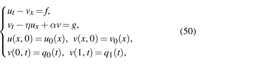
Let $Ω = [0, L]$ and $\tilde{Ω} = Ω \times (0, \infty)$ . Consider the system

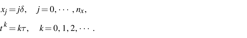
\begin{matrix} {\begin{matrix} u_{t} - v_{x} = f, \\ v_{t} - η u_{x} + αv = g, \\ u (x, 0) = u_{0} (x), v (x, 0) = v_{0} (x), \\ v (0, t) = q_{0} (t), v (1, t) = q_{1} (t), \end{matrix} \end{matrix}

(50)

for all $(x, t) \in \tilde{Ω}$ . Let τ be a time step, and $δ = \frac{L}{n_{x}}$ be a spatial step. Then, any grid point $(x_{j}, t^{k}) \in \tilde{Ω}$ is defined by

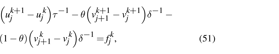
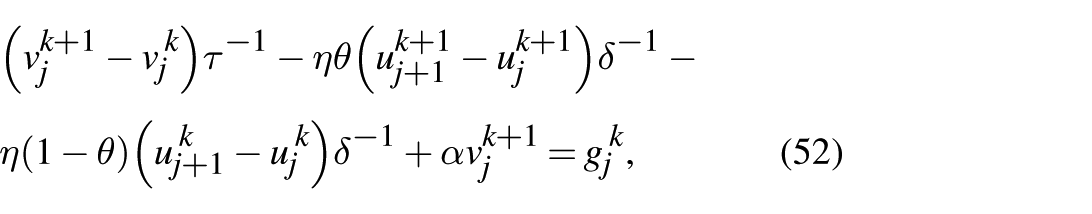
\begin{matrix} x_{j} = & jδ, j = 0, \dots, n_{x}, \\ t^{k} = & kτ, k = 0, 1, 2, \dots . \end{matrix}

A finite difference θ-scheme (Arfaoui, 2020) has been used for the discretization of the problem (50). So, at the grid point $(x_{j}, t^{k})$ , we have

\begin{matrix} (u_{j}^{k + 1} - u_{j}^{k}) τ^{- 1} - θ (v_{j + 1}^{k + 1} - v_{j}^{k + 1}) δ^{- 1} - \\ (1 - θ) (v_{j + 1}^{k} - v_{j}^{k}) δ^{- 1} = f_{j}^{k}, \end{matrix}

(51)

\begin{matrix} (v_{j}^{k + 1} - v_{j}^{k}) τ^{- 1} - ηθ (u_{j + 1}^{k + 1} - u_{j}^{k + 1}) δ^{- 1} - \\ η (1 - θ) (u_{j + 1}^{k} - u_{j}^{k}) δ^{- 1} + α v_{j}^{k + 1} = g_{j}^{k}, \end{matrix}

(52)

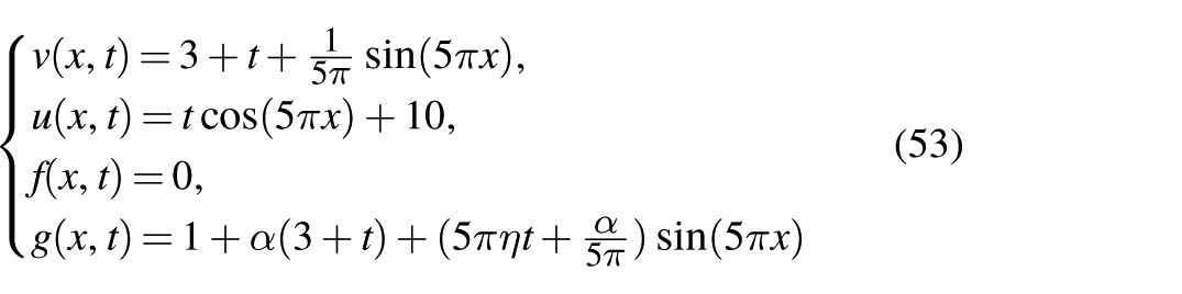
where $v_{j}^{k} = v (x_{j}, t^{k})$ and $u_{j}^{k} = u (x_{j}, t^{k})$ , for all $j = 0, \dots, n_{x}$ and $k = 0, 1, 2, \dots$ . Note that the θ-scheme is unconditionally stable for $θ \in [0.5, 1]$ . In fact, this scheme is well adapted for the hyperbolic systems. Let $η = 3$ and $α = 2$ . To validate the numerical method, we choose the exact solutions $v (x, t)$ and $u (x, t)$ , for all $(x, t) \in [0, 1] \times [0, 1.5]$ , as follows

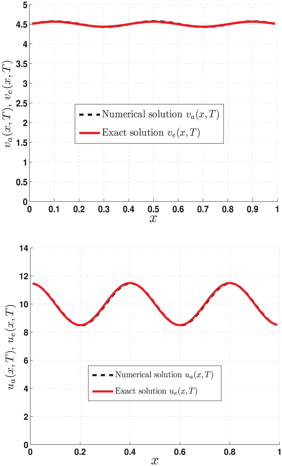
\begin{matrix} {\begin{matrix} v (x, t) = 3 + t + \frac{1}{5 π} \sin (5 πx), \\ u (x, t) = t \cos (5 πx) + 10, \\ f (x, t) = 0, \\ g (x, t) = 1 + α (3 + t) + (5 πηt + \frac{α}{5 π}) \sin (5 πx) \end{matrix} \end{matrix}

(53)

In Figure 1, we plotted the numerical solutions $v_{a} (x, T)$ and $u_{a} (x, T)$ , and the exact solutions $v_{e} (x, T)$ and $u_{e} (x, T)$ , for $T = 1.5$ . The relative errors between the numerical solutions and the exact solutions are

\begin{matrix} e_{r}^{v} (t) = & \frac{∥ v_{e} (\cdot, t) - v_{a} (\cdot, t) ∥_{\infty}}{∥ v_{e} (\cdot, t) ∥_{\infty}}, \end{matrix}

(54)

\begin{matrix} e_{r}^{u} (t) = & \frac{∥ u_{e} (\cdot, t) - u_{a} (\cdot, t) ∥_{\infty}}{∥ u_{e} (\cdot, t) ∥_{\infty}} . \end{matrix}

(55)

Figure 1.

The numerical solutions $v_{a} (x, T)$ and $u_{a} (x, T)$ , and the exact solutions $v_{e} (x, T)$ and $u_{e} (x, T)$ , for $T = 1.5$ .

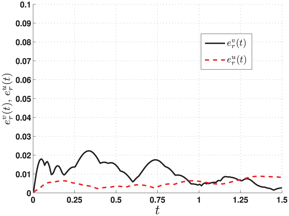
In Figure 2, the relative errors defined in (54)–(55) were plotted for $t \in [0, 1.5]$ . Therefore, we conclude that the numerical methods (51) and (52) are well suited to the numerical resolution of the hyperbolic system (50).

Figure 2.

The relative errors $e_{r}^{v} (t)$ and $e_{r}^{u} (t)$ , for $t \in [0, 1.5]$ .

Numerical experiments

Let $Ω = (0, 1)$ . Consider the linear non-homogeneous Dirichlet boundary system

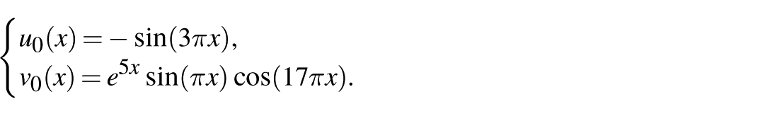
\begin{matrix} {\begin{matrix} u_{t} - v_{x} = 0, \\ v_{t} - η u_{x} + αv = f (x) u (0, t), \\ u (x, 0) = u_{0} (x), v (x, 0) = v_{0} (x), \\ v (0, t) = 0, v (1, t) = q_{1} (t), \end{matrix} \end{matrix}

(56)

for all $(x, t) \in Ω \times (0, \infty)$ . The initial conditions $u_{0} (x)$ and $v_{0} (x)$ , for $0 \leq x \leq 1$ , are given as follows

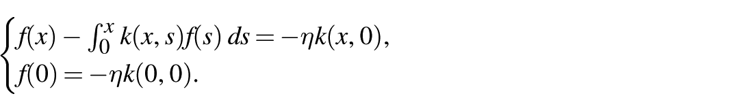
\begin{matrix} {\begin{matrix} u_{0} (x) = - \sin (3 πx), \\ v_{0} (x) = e^{5 x} \sin (πx) \cos (17 πx) . \end{matrix} \end{matrix}

The kernel function $k (x, s)$ is given explicitly as follows

\begin{matrix} k (x, s) = 8 \cos (e^{3 (x - s)}), 0 \leq s \leq x \leq 1 . \end{matrix}

(57)

Remark that $k (x, s)$ satisfies the first equation of system (28). Now, we can determine the function $f (x)$ , defined in system (56), through the numerical resolution of the following integral equation, which is derived from the system (28)

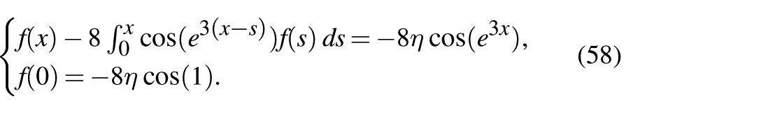
\begin{matrix} {\begin{matrix} f (x) - \int_{0}^{x} k (x, s) f (s) ds = - ηk (x, 0), \\ f (0) = - ηk (0, 0) . \end{matrix} \end{matrix}

for $0 \leq x \leq 1$ . Using expression (57), we get

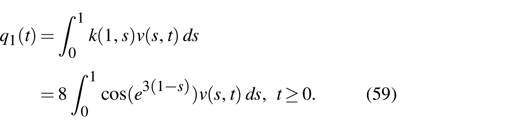
\begin{matrix} {\begin{matrix} f (x) - 8 \int_{0}^{x} \cos (e^{3 (x - s)}) f (s) ds = - 8 η \cos (e^{3 x}), \\ f (0) = - 8 η \cos (1) . \end{matrix} \end{matrix}

(58)

for $0 \leq x \leq 1$ . Using again expression (57), the feedback control law $q_{1} (t)$ , see (45), takes the following form

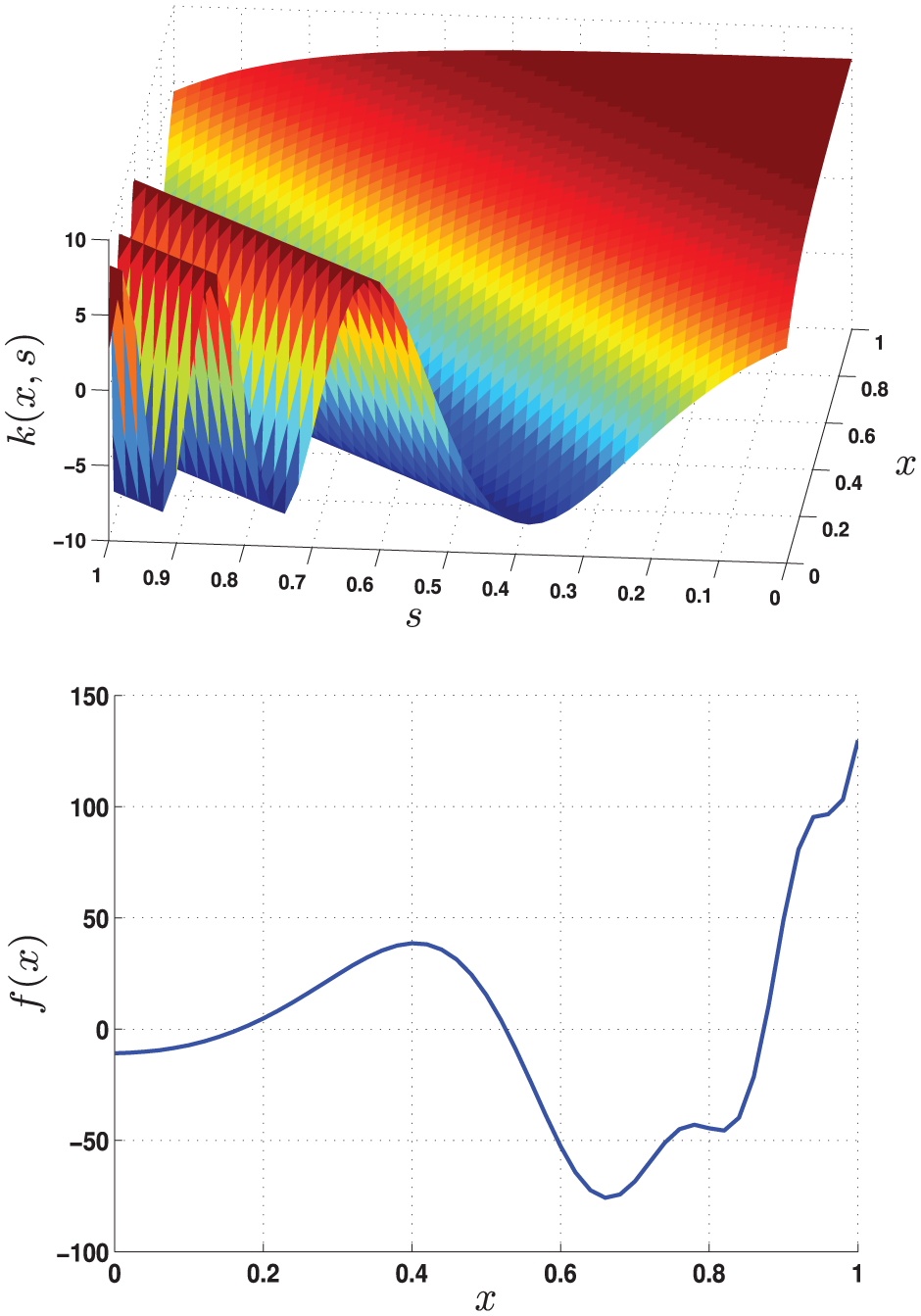
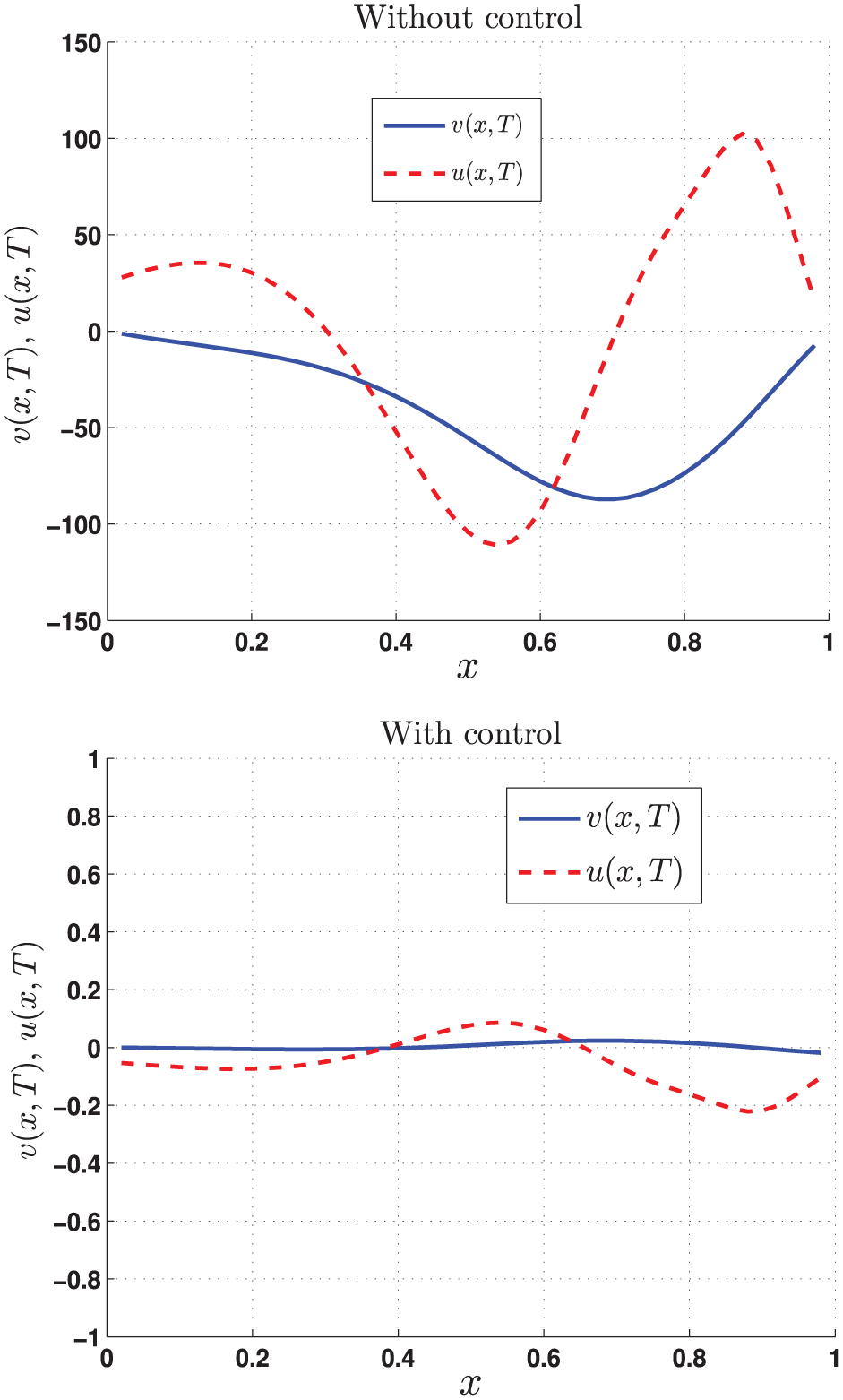
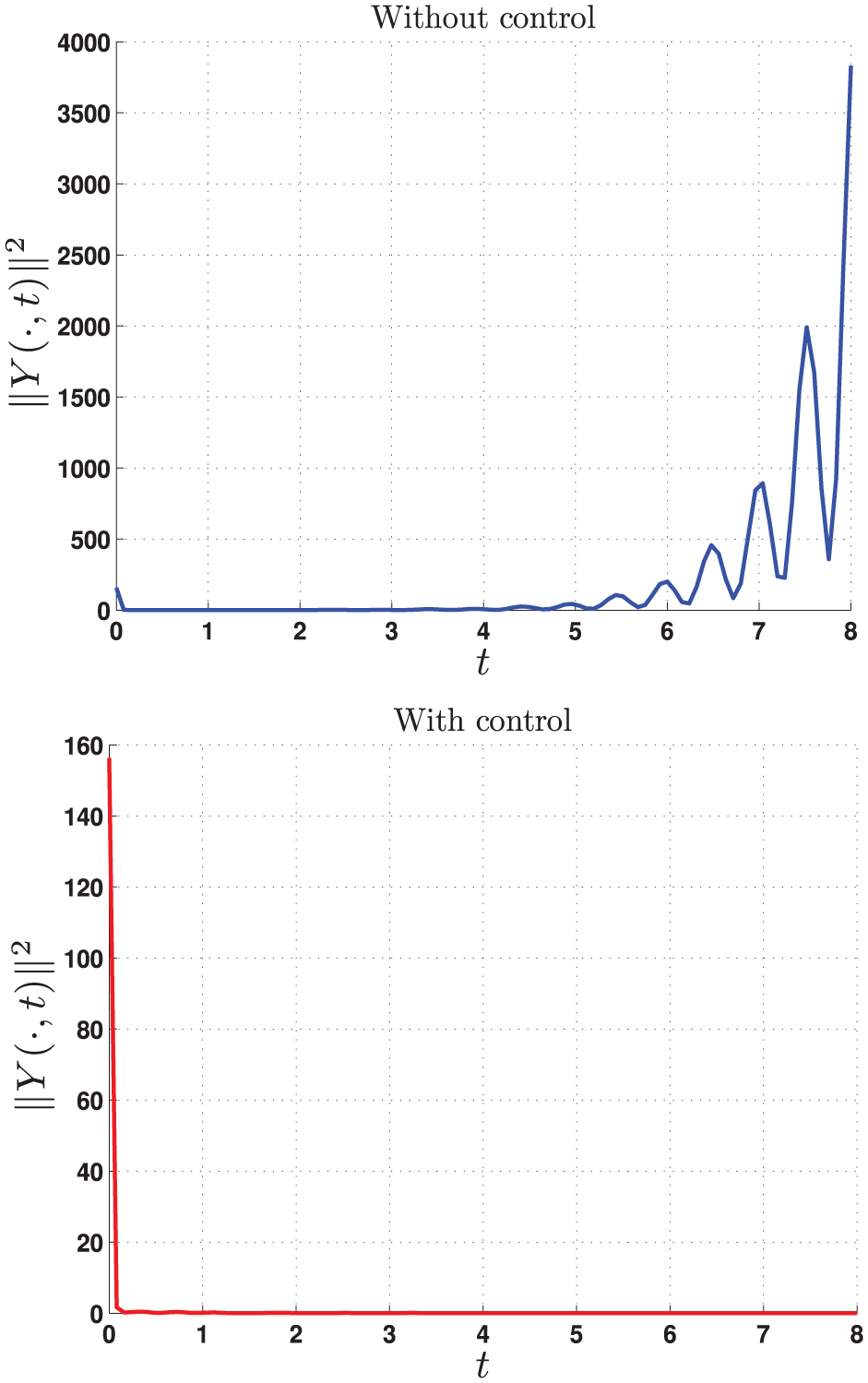
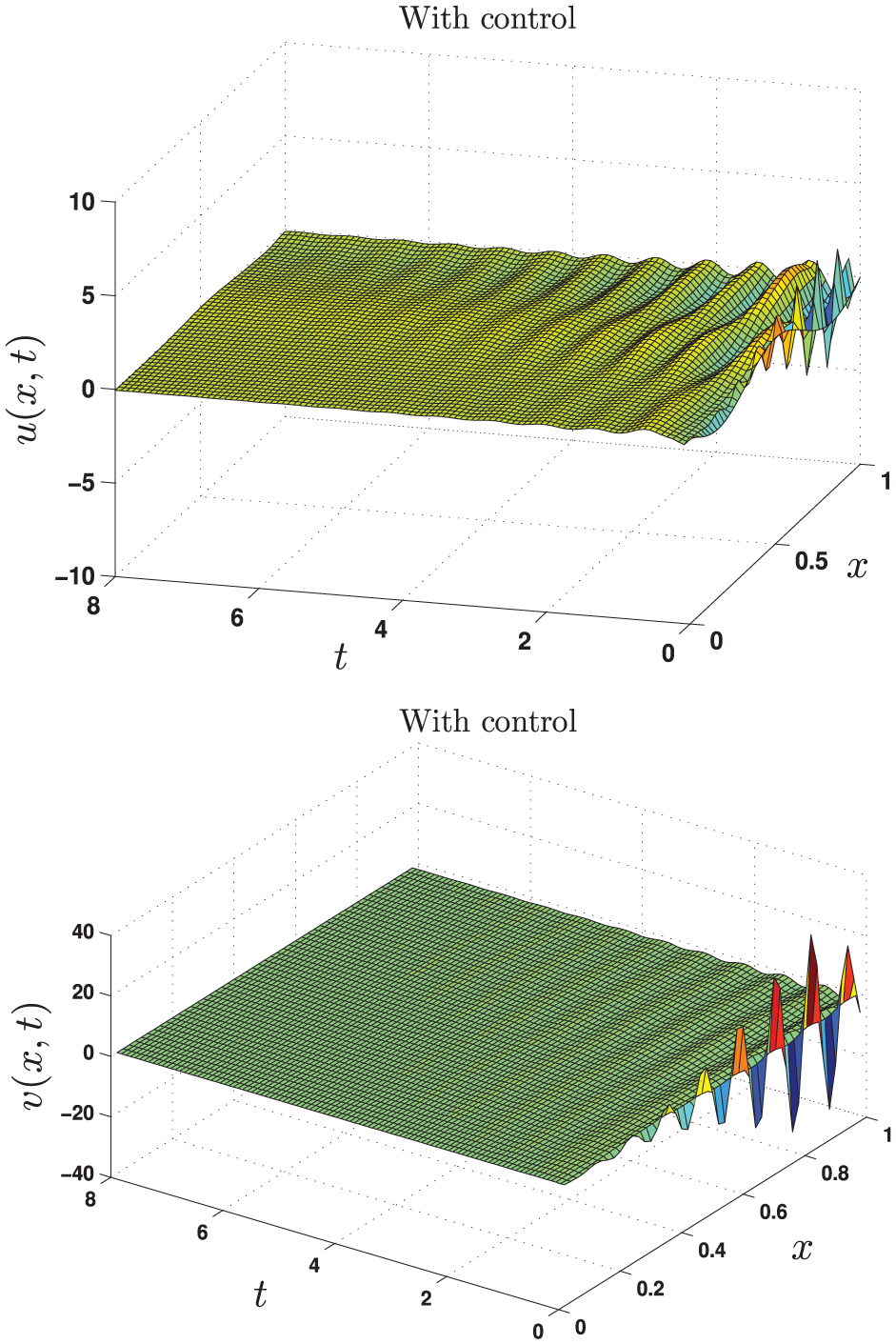
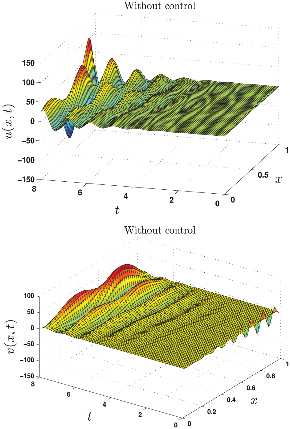
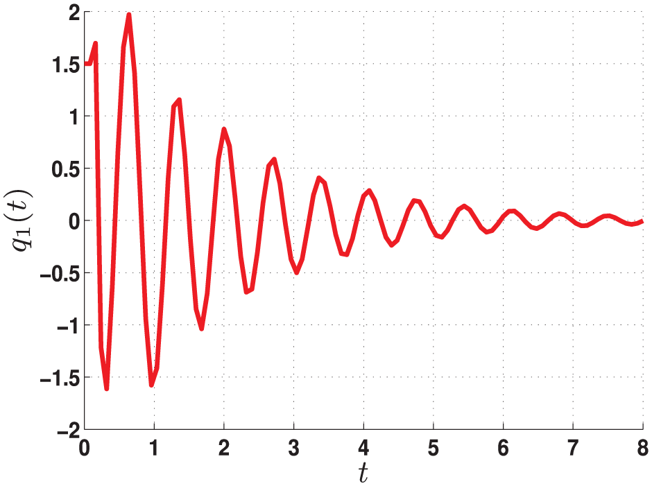
\begin{matrix} q_{1} (t) = & \int_{0}^{1} k (1, s) v (s, t) ds \\ = 8 \int_{0}^{1} \cos (e^{3 (1 - s)}) v (s, t) ds, t \geq 0 . \end{matrix}

(59)

For the numerical experiments, consider the following data: $α = 1$ , $η = 2.5$ . In Figure 3, we have plotted the curve of the function $f (x)$ obtained from the system (58). The function $f (x)$ will be used for the numerical simulation of the closed-loop systems (56) and (59). Figures 4 and 7 show the instability of the solution $u (x, t)$ and $v (x, t)$ for $T = 8$ . While Figures 4 –6 confirm the theoretical result established in Theorem 5. Indeed, the norm of the solution $Y = (u, v)$ tends to zero for $T = 8$ . Thus, the feedback control law (59) has accelerated the stabilization of the system (56). Figure 8 represents the feedback control law $q_{1} (t)$ , for $t \in [0, 8]$ .

Figure 3.

The kernel function $k (x, s)$ and the function $f (x)$ for $0 \leq s \leq x \leq 1$ .

Figure 4.

The solutions $u (x, t)$ and $v (x, t)$ plotted without control, for $(x, t) \in [0, 1] \times [0, 8]$ .

Figure 5.

The solutions $v (x, T)$ and $u (x, T)$ plotted with and without control, for $x \in [0, 1]$ and $T = 8$ .

Figure 6.

The solutions $u (x, t)$ and $v (x, t)$ plotted with control, for $(x, t) \in [0, 1] \times [0, 8]$ .

Figure 7.

The norm of the solutions $∥ Y (\cdot, t) ∥^{2}$ plotted without and with control, for $t \in [0, 8]$ .

Figure 8.

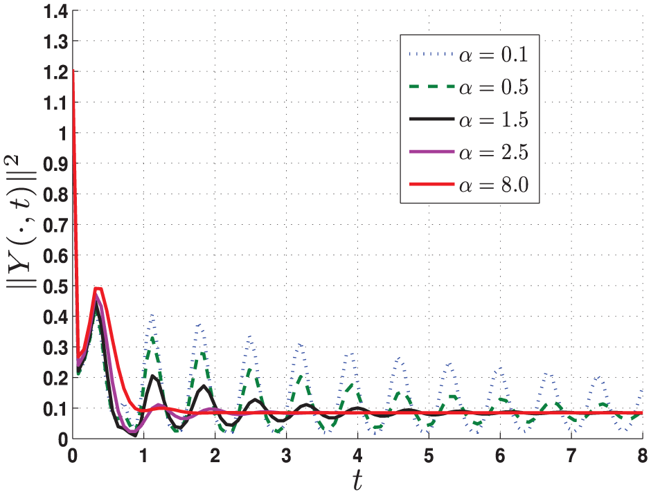
The feedback control law $q_{1} (t) = 8 \int_{0}^{1} \cos (e^{3 (1 - s)}) v (s, t) ds$ , for $0 \leq t \leq 8$ .

In Figure 9, we discussed the behavior of the exponential stabilization of the solution with respect to the decay rate $(- α)$ given by Theorem 5. In fact, this example agrees perfectly with the stability identity (49), since increasing the value of α leads to a fast stabilization of the solution. Note that to obtain Figure 9, we only changed the initial condition associated with the state v, where we took $v_{0} (x) = 10 e^{- 5 x} \sin (πx) \cos (17 πx)$ , keeping all other data fixed. In fact, this change aims to have a clearer and more readable figure.

Figure 9.

Behavior of the exponential stabilization of the solution with respect to the decay rate $(- α)$ given by Theorem 5.

Conclusion and perspective

In this work, we have achieved interesting objectives, including the stabilization of the LHS through Dirichlet boundary feedback control. The backstepping transformation is used in constructing the state feedback law. This control allows for obtaining an exponential stability result for the LHS with a fixed decay rate equal to $(- α)$ (α is in system (12)). In the second part of this work, the numerical implementation and interpretation of the results were discussed. First, we have proposed and validated a numerical method for the numerical resolution of the closed-loop system. Then, we gave practical examples which show, on the one hand, the effectiveness of the feedback control law designed for the stabilization of the system and, on the other hand, confirm the theoretical results obtained.

A very important question that can be asked: can the feedback law designed for the linearized system be applied to stabilize the nonlinear system? Also, one can consider an in-depth discussion on the observability and controllability of the LHS. Again, in this context, we can perform a thorough analysis of fractional systems.

Footnotes

ORCID iDs

Hassen Arfaoui

Feten Maddouri

Ethical approval and informed consent

We affirm that this manuscript is original, has not been published before, and is not currently being considered for publication elsewhere.

Author contributions

Hassen Arfaoui: Conceptualization; Validation; Software; Writing—original draft.

Feten Maddouri: Conceptualization; investigation; resources; Writing—original draft.

Funding

The authors received no financial support for the research, authorship, and/or publication of this article.

Declaration of conflicting interests

The authors declared no potential conflicts of interest with respect to the research, authorship, and/or publication of this article.

Data availability statement

Data sharing is not applicable to this article, as no new data were created or analyzed in this study.

References

Aamo

(2006) Disturbance rejection in 2x2 linear hyperbolic systems. IEEE Transactions on Automatic Control 58: 1095–1106.

Amaury

(2021) Boundary stabilization of 1D hyperbolic systems. Annual Reviews in Control 52: 222–242.

Arfaoui

(2020) Stabilization method for the Saint-Venant equations by boundary control. Transactions of the Institute of Measurement and Control 42(16): 3290–3302.

Castillo

Witrant

Dugard

(2013a) Dynamic boundary stabilization of linear parameter varying hyperbolic systems: Application to a Poiseuille flow. In: Proceedings of the 11th IFAC workshop on time-delay systems, Grenoble, France, February 4–6.

Castillo

Witrant

Prieur

, et al. (2013b) Boundary observers for linear and quasi-linear hyperbolic systems with application to flow control. Automatica 49(11): 3180–3188.

Castillo

Witrant

Prieur

, et al. (2016) Dynamic boundary stabilization of first order hyperbolic systems. In: Witrant

Fridman

Sename

, et al. (eds) Recent Results on Time-Delay Systems. Advances in Delays and Dynamics, volume 5. pp. 169–190. Springer, Cham. https://doi.org/10.1007/978-3-319-26369-4\_9

Chowdhury

Dutta

Majumdar

(2021) Boundary stabilizability of the linearized compressible Navier-Stokes system in one dimension by backstepping approach. SIAM Journal on Control and Optimization 59(3): 2147–2173.

Coron

Guillaume

, et al. (2021) Boundary stabilization in finite time of one-dimensional linear hyperbolic balance laws with coefficients depending on time and space. Journal of Differential Equations 271: 1109–1170.

Krstic

Smyshlyaev

(2008) Backstepping boundary control for first-order hyperbolic PDEs and application to systems with actuator and sensor delays. Systems and Control Letters 57(9): 750–758.

10.

Liu

(2022) Boundary feedback stabilization of an unstable heat equation. SIAM Journal on Control and Optimization 42(3): 1033–1043.

11.

Maddouri

(2024) On the stability of the linearized compressible adiabatic flow through porous media. Filomat 38(13): 4585–4595.

12.

Maracati

Pan

(2001) On the diffusive profiles for the system of compressible adiabatic flow through porous media. SIAM Journal on Mathematical Analysis 33(4): 790–826.

13.

Zhou

Guo

(2018) Boundary feedback stabilization for an unstable time fractional reaction diffusion equation. SIAM Journal on Control and Optimization 56(1): 75–101.