
Abstract
In cross-domain bearing fault diagnosis, the lack of labeled samples in the target domain requires models to transfer knowledge from a labeled source domain. However, differences in operating conditions lead to domain drift between domains, and conventional global alignment methods may further introduce inter-class confusion, degrading diagnostic performance. In addition, in complex and variable application scenarios, it is difficult to ensure the availability of sufficient samples for training deep learning diagnostic models. To overcome these challenges, this paper proposes a residual network with a domain adaptation mechanism. First, the local maximum mean discrepancy (LMMD) is adopted as a metric to describe the feature variations between the source and target domains. Through feature distribution alignment of the same fault type in the relevant subdomains, the offset of the local domain is derived for the cross-domain cases. By introducing LMMD into a so-called domain adaptation layer, the unexpected feature difference for the same bearing fault type can be minimized in a high-dimensional feature space. Second, the residual network with dense connections is used as the backbone to represent the local and global features of the bearing faults completely. This network takes the RGB image transformed from the time-sequence signal as the input and strengthens global feature extraction through dense parallel connections. Finally, the effectiveness of the proposed method was validated on the Case Western Reserve University (CWRU) dataset and the Paderborn dataset. Experimental results have shown that the proposed network achieves high prediction accuracy in cross-domain bearing fault diagnosis.
Introduction
The rolling bearing is a crucial component of mechanical machinery, and unexpected failure events of the bearing, such as peeling off and wear, can endanger the safe and stable operation of the entire mechanical system (Chen et al., 2020a). Hence, effective bearing fault diagnosis is critical for ensuring the health of the machinery. Traditional data-driven diagnostic methods rely highly on manually selected, shallow features. They cannot easily tackle complex diagnostic problems, such as cases involving various loads and noise interference (Report, 1987). Deep learning (DL) networks can diagnose bearing faults by using deep hierarchical networks to adaptively extract multilevel features and automatically classify the fault types (Tang et al., 2021). Many attempts were made to apply the DL networks to bearing fault diagnosis and classification.
Based on DL architecture, the convolutional neural networks (CNNs), which are specifically designed for variable and complex signals, have shown great merits in extracting the features of bearing faults (Li and Zhang, 2021; Wang et al., 2022; Zhu et al., 2021a). In the real-world industrial environment, inconsistent working loads, input feature variation, and unbalanced data can easily cause the overfitting of the CNN. The derived diagnostic model delivers better performance on the source domain samples but poorer generalization on the target domain samples. Transfer learning methods can partially solve this problem, but they still have limitations, which are rooted in the structure of the CNN (Ren et al., 2021). The CNN mechanism does not consider sequential features—the natural characteristics of the time series of vibration signals. The local receptive field of the convolutional kernel requires the stacking of layers to obtain global information. It is still difficult to capture the long-term dependency between the sampling signal points, even if the convolutional kernels are designed to be sufficiently large to cover ample data points (Song et al., 2022). In addition, constrained by the limited depth, a CNN-based diagnosis model such as ResNet18 (He et al., 2016) can only capture clusters of regional features, making the CNN vulnerable to feature-distribution variation subject to a cross-domain condition.
Extracting sufficient local and global information is critical for ensuring good fault diagnostic performance. At the same time, feature extraction should remain robust under various working conditions where the training data and the testing data are in different distribution spaces and have different marginal distributions. Many researchers have attempted to improve DL networks from different perspectives to enhance model-feature-extraction capabilities and to maintain robustness in different application scenarios. Liang et al. (2022) employed multi-scale convolutions in a residual network. The weights of multi-scale convolution layers were dynamically adjusted by the attention mechanism. Then, the feature-extraction ability of the diagnostic model was enhanced by inputting supplementary feature information. Diagnosis accuracy degradation due to the cross-domain distribution discrepancy was effectively alleviated. Instead of the attention mechanism, Du et al. (2020) combined transfer learning with deep residual networks to compensate for the cross-domain imbalance discrepancy. After full training on a multitude of source domain samples, the networks were further fine-tuned to adapt to the target feature distribution with labeled target domain samples. Xu et al. (2023) proposed a densely connected deep residual network (DDRN) model based on ResNet. In this DDRN model, additional parallel dense connections were added between the residual blocks to merge and transfer the features of different depths. The proposed DDRN realized robust feature extraction under various working conditions. However, it still requires labeled samples from the target domain to make specific adjustments to the model parameters. For the cross-domain diagnosis of unlabeled samples in the target domain, Zhao et al. (2021) used the maximum mean discrepancy (MMD) to minimize the feature difference between the source and target domains. Then, the global domain-invariant features were derived from a quantified feature difference across the working states. However, this global domain adaptation method did not consider the relationship between the individual classes in the two domains.
Limitations of global alignment have motivated the development of methods capable of capturing finer-grained data structures. At the same time, graph contrastive learning (GCL) methods (Xie et al., 2021), which leverage contrastive loss and mutual information maximization to learn invariant representations within data, have achieved remarkable success. Representative works include GraphCL (Hafidi et al., 2020), Deep Graph Infomax (DGI) (Velickovic et al., 2018), and SimGRACE (Xia et al., 2022). GraphCL applies multiple graph-augmentation techniques and InfoNCE loss to maximize the consistency of representations across views; however, its performance highly depends on augmentation strategies specifically designed for graph structures. DGI employs a discriminator to maximize mutual information between local node representations and the global graph summary but lacks mechanisms to learn fine-grained category-discriminative features. SimGRACE generates views by perturbing encoder parameters, thereby avoiding complex graph augmentations, but the perturbation mechanism lacks explicit semantic guidance, making it difficult to ensure semantic consistency of the generated views at the category level. A common premise of these GCL methods is that the input data inherently possess graph structures, with the primary objective being the learning of graph- or node-level representations. Despite their notable performance in respective domains, their design focuses on instance-level invariance and graph-level representation learning without incorporating explicit class-conditional cross-domain alignment mechanisms. Consequently, direct application to the present study would be ineffective in addressing the core challenge of aligning same-class data across domains, potentially leading to inter-class confusion (Shen et al., 2022).
Building on these efforts, several other studies have explored advanced transfer learning techniques for cross-domain bearing fault diagnosis. A large number of studies have already focused on cross-domain bearing fault diagnosis. Chen et al. proposed a Domain Adversarial Transfer Network (DATN) to address the large distribution discrepancies in cross-domain fault diagnosis for rotary machinery (Chen et al., 2020b). This method employs asymmetric encoder networks based on deep CNNs to extract hierarchical representations from source and target domains, while using domain adversarial training to minimize distribution differences. By aligning features adversarial, it handles domain shifts effectively, achieving improved diagnostic accuracy and robustness in mismatched operating conditions. Shao and Kim proposed an Adaptive Multi-Scale Attention Convolutional Neural Network (AmaCNN) to accurately detect cross-domain faults in mechanical systems with very few labeled data (Shao and Kim, 2024). The approach extracts multi-scale less-noise features using multi-scale feature fusion CNN with a multi-level attention scheme and aligns domains through correlation alignment and semantic consistency to reduce distribution gaps. This enables effective knowledge transfer across domains, resulting in enhanced fault diagnosis performance and higher precision in variable environments. To achieve intelligent fault diagnosis for bearings under frequent impacts and complex working conditions, Ning et al. proposed a digital twin-driven cross-domain adaptation method (Ning et al., 2025). It leverages digital twins to simulate and generate labeled source samples for transfer learning, thereby bridging domain gaps by adapting simulated data to real-world scenarios. This facilitates robust fault identification without extensive real labeled data, leading to improved diagnostic reliability and efficiency in applications such as aerospace, railways, and wind turbines. Zhang et al. proposed a cross-domain decision method based on Instance Transfer and Model Transfer (WSER) to facilitate knowledge transfer in fault diagnosis with limited data and distribution dissimilarities (Zhang et al., 2024). The method extracts features from time, frequency, and time-frequency domains; estimates data weights via instance transfer to mitigate distribution differences; and transfers knowledge from source models using decision trees with structure expansion and reduction. This approach effectively reduces domain gaps and enhances fault classification, demonstrating superior performance in cross-domain scenarios with sparse labels. Tang et al. proposed the Continuous Wavelet Transform - SimAM - Domain Adaptation with Adaptive Weighting Strategy (CWT-SimAM-DAMS) method to address the challenges of domain shift in bearing fault diagnosis under complex conditions with dispersed data and distinct distribution differences (Tang et al., 2024). This approach employs Continuous Wavelet Transform (CWT) and unsharp masking (USM) for data preprocessing to enhance feature contrast in weak signals, integrates the SimAM module into ResNet for improved feature extraction without additional parameters, and uses an adaptive weighting strategy based on Joint Maximum Mean Discrepancy (JMMD) and Conditional Adversarial Domain Adaptation Network (CDAN) to minimize distribution differences between source and target domains. By combining these elements, it effectively handles non-linear distributions and noise interference, achieving higher diagnostic accuracy on two datasets. Although these methods offer significant benefits in advancing domain alignment, feature extraction, and knowledge transfer for fault diagnosis, thereby improving diagnostic accuracy and robustness in various cross-domain scenarios, they may exhibit limitations in fully addressing fine-grained class-level subdomain alignment and robust integration of global and local features, particularly in unsupervised scenarios with unlabeled target domains and varying noise interference.
Despite these advancements in transfer learning techniques, practical industrial scenarios still face significant challenges due to domain drift caused by varying operating conditions, such as speed and load. This often results in inter-class confusion from global distribution alignment, making class-aware cross-domain adaptation a critical issue for reliable bearing fault diagnosis.
Meanwhile, in practical industrial scenarios, labeled fault samples are usually scarce in the target domain, which makes it difficult to train reliable diagnostic models directly. As a result, cross-domain transfer learning has become an effective solution for bearing fault diagnosis. However, differences in operating conditions such as speed and load lead to domain drift between source and target domains. Existing domain adaptation methods typically perform global distribution alignment, which may inadvertently mix features from different fault categories and result in inter-class confusion. Therefore, how to achieve class-aware cross-domain alignment under domain drift becomes the key challenge for reliable bearing fault diagnosis.
To address the issue of inter-class confusion in cross-domain diagnosis, a novel cross-domain diagnostic approach targeting unlabeled samples in the target domain is proposed. This approach effectively avoids the inter-class confusion inherent to traditional global adaptation methods and graph contrastive approaches lacking a category-alignment mechanism. To achieve this goal, a domain adaptation mechanism combining local maximum mean discrepancy (LMMD) and a DDRN was designed. By aligning the distributions of subdomains corresponding to the same fault categories in the source and target domains, the accuracy of cross-domain bearing fault diagnosis is significantly improved.
The three main contributions of this study can be summarized as follows:
LMMD is employed as a category-conditioned domain adapter to minimize distribution differences between corresponding subdomains in the source and target domains, thereby effectively mitigating the inter-class confusion that may arise when using global MMD.
A ResNet-based backbone network featuring dense connections (DDRN) is proposed to enhance feature-extraction performance by integrating global and local feature information, thereby improving the capability of the model to identify bearing faults.
LMMD and DDRN are integrated into an end-to-end model, referred to as LMMD–DDRN, which aligns feature distributions in high-dimensional feature space to minimize cross-domain discrepancies, addressing the unsupervised domain adaptation problem in bearing fault diagnosis.
The rest of this article is organized as follows. The Problem description and theoretical knowledge section summarizes the domain drift problem in cross-domain diagnostic tasks and the LMMD for measuring feature variations. The ResNet with dense connections and RGB image input section briefly describes the construction of the DDRN and its RGB mapping input, which is used for global feature reinforcement from the perspective of supplementing feature information. The Cross-domain fault diagnostic model with the LMMD domain adaptor section describes the derivation of the DDRN diagnostic model with an LMMD domain adaptor for rolling bearing faults. The Experimental results and discussion section provides the cross-domain diagnosis results of the proposed approach on both the Case Western Reserve University (CWRU) and Paderborn datasets. The final section provides the conclusions and discusses the possible future work.
Problem description and theoretical knowledge
Domain drift of feature representation
In practical industrial scenarios, different operating conditions lead to different probability distributions of the fault samples. The consequent domain shift in the representative characteristics of the faults causes a bottleneck in the diagnostic model for the cross-domain diagnostic tasks.
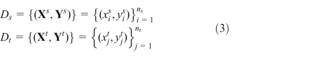
The sample spaces defined on the source and target domains are denoted by

Here, n
s
and n
t
are the sample numbers in the source and target domains, respectively. Meanwhile, the corresponding labels assigned to the samples

Then, the available datasets from the source and target domains can be described as
with
When the operating condition of the bearing changes in terms of speed and load torque according to various tasks, the marginal probability distributions of the vibration signals differ, though they belong to the same object.

where
Consequently, the conditional probability distribution in the source domain encounters an inconsistency with the target domain.

For the cross-domain diagnosis of the bearing fault, the diagnosis model works under the prerequisite that the vibration signals collected from different working states have the same fault label

The domain shift in the distribution between the source and target domain data will cause deterioration of the accuracy of the diagnostic model. As shown in Figure 1, two types of bearing faults were considered in the source and target domains. The domain classifier, a type of diagnostic model, was obtained via learning from the source domain. Because of the lack of cross-domain distribution consistency, the fault types may be misclassified when the domain classifier is applied directly to the target domain. As shown in Figure 1(a), although the two fault types have different feature representations, the domain classifier cannot distinguish between them. In the low-level feature space constructed by the superposition of the source and target domains, the two feature representations are confused and indistinguishable.
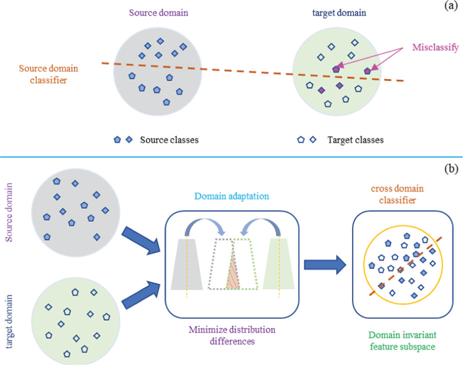
Cross-domain classification methods: (a) traditional low-level feature-based methods and (b) domain adaptation–based methods.
The MMD-based global feature-adaptation method can solve the domain shift due to the cross-domain distribution difference (Pan et al., 2020). The feature representations in the source and target domains are mapped into the same feature space through a transformation function φ(.). In this high-level space, the MMD is adopted to measure and minimize the distance between

Then, a cross-domain diagnostic model is derived that aligns the probability distribution across domains based on a domain adaptation strategy. As shown in Figure 1(b), in a domain-invariant feature subspace obtained after conditional probability distribution adaptation, the feature representations of the same label cluster facilitate the cross-domain classifier to complete the fault classification.
Local MMD
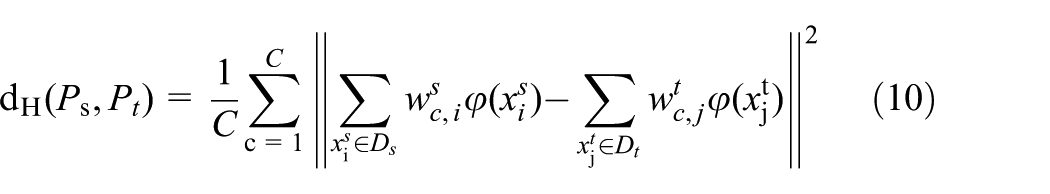
MMD focuses on aligning the global feature distribution and measures the differences in the distributions of two working domains of the rolling bearing. The measurement criterion dH is determined by the squared expectation gap between two independent variables on an expanded high-level feature space, as shown below

where φ(.) is used to map the original samples to the reproducing kernel Hilbert space.
The MMD approach does not consider the relationship between different classes in the respective domains and may lead to data confusion between domains. As shown in Figure 2(a), after the global domain adaptation by MMD, the two domains assume roughly the same probability distribution. However, the data distributions of different classes are too close, hindering accurate classification. To solve this problem, the feature conformity between subdomains in different domains should be considered. Subdomains are predefined based on class label information, and samples of the same category are classified into one subdomain. They are adopted to align the feature representations in the relevant subdomains based on the LMMD (Zhu et al., 2021b).
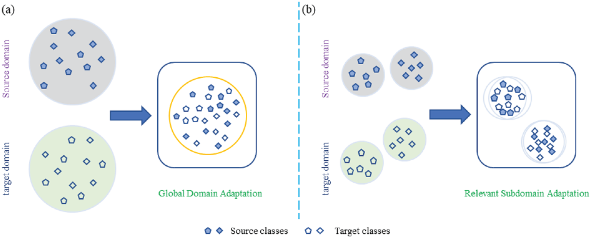
Subdomain adaptation for cross-domain classification: (a) global domain adaptation classification and (b) subdomain adaptation classification.
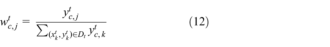
The measurement criterion is rewritten as

where C is the present number of subdomains, which is exactly the number of the categories of the bearing fault type;
In practical applications, the mathematical expectation can be equivalently realized by a weighted membership of the samples in the subdomains. Then, the measurement criterion is determined by
where
The weight
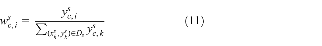
The weight
In the traditional cross-domain classification where the target domain samples have designated labels, their membership to a given class can be obtained through equation (11). However, for unknown target domain samples, there is no corresponding label information.
This study uses the universal approximation of the deep neural networks, a CNN network, that is, the DDRN, is used to generate an estimated label
where
For the DDRN, a dense connection is introduced in the deep residual network to supplement the global feature information and guarantee sufficient and robust feature extraction of the bearing fault.
ResNet with dense connections and RGB image input
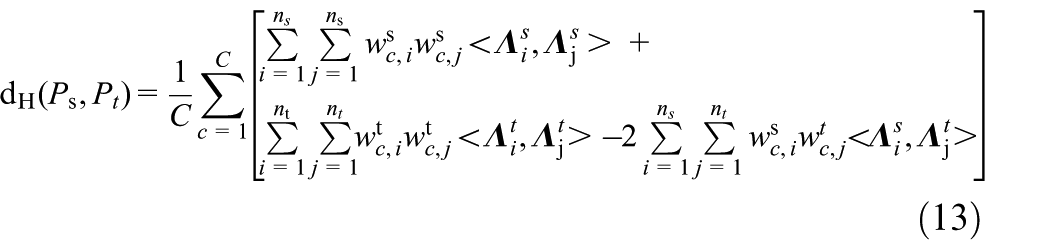
The complete representation of the local and global features of the bearing faults is an essential prerequisite for cross-domain diagnosis. Traditional deep networks cause the abatement of global information by the deepening of layers. From the viewpoint of the global feature-extraction promotion of the model, the so-called DDRN in Xu et al. (2023) is introduced as the backbone for feature encoding of the bearing faults. As shown in Figure 3, DDRN takes serially connected multiple ResNet layers to extract and fuse the deep features, while additional dense connections are added across layers to retain the global features during the deepening of the networks. Meanwhile, the DDRN takes the RGB image transformed from the time-series vibration signals as its input. The RGB images are generated by a differential operation on the time-domain series, capable of considering the distance-related characteristics of the vibration signal.
Structure of the DDRN.

where

Then, by using the preactivation layer σ(.) to reduce the dimension and average pooling AvPooling(.) for size reduction, DDRN provides a type of complete features of the bearing faults

Cross-domain fault diagnostic model with the LMMD domain adaptor
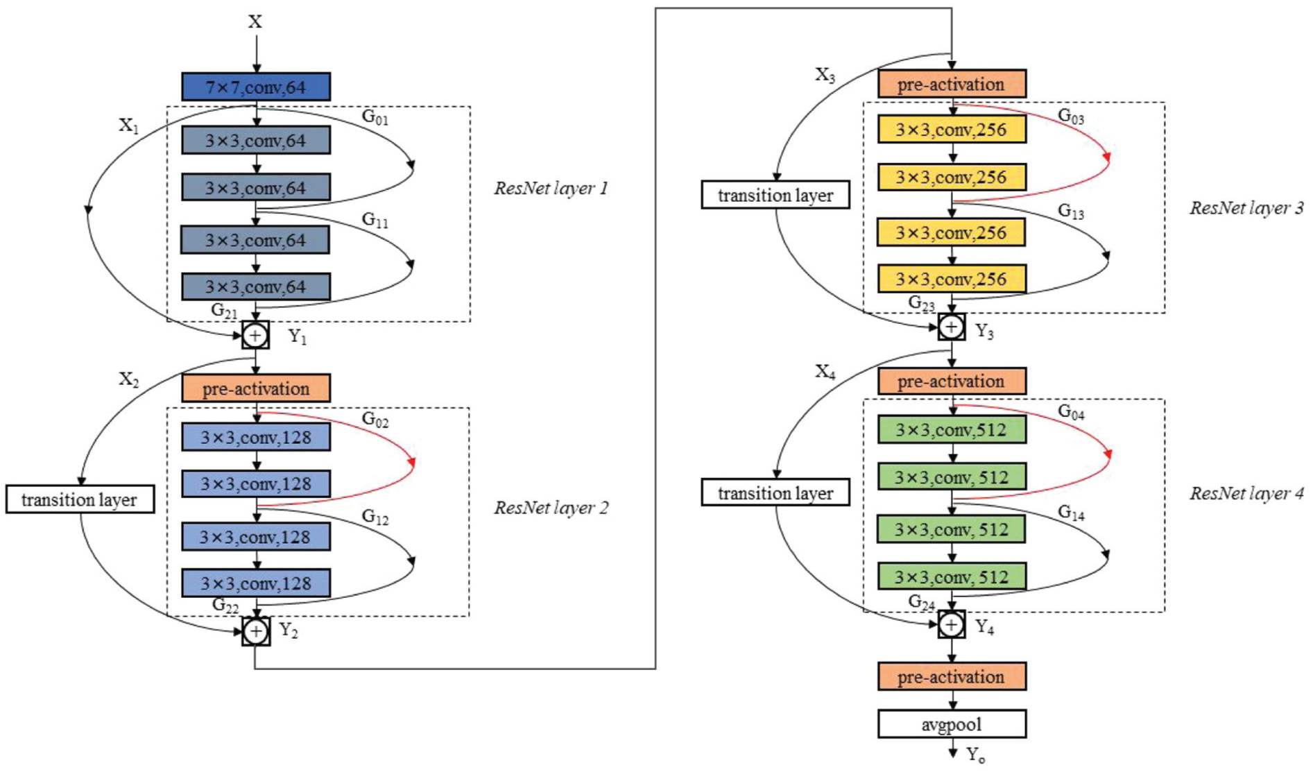
A schematic diagram of the cross-domain fault diagnosis model, named LMMD–DDRN, is shown in Figure 4. The model takes the one-dimensional vibration signal as its input. Xu et al. (2023) adopted the same signal-processing method, and the RGB image converted from the time series was used for the DDRN input. The DDRN is used as the feature extractor for the bearing fault, and samples from both the source and target domains are taken simultaneously as input. The source domain samples with labels provide diagnostic information for model training, while the DDRN estimates the class of the samples in the target domain through the trained model. With the introduction of the LMMD domain adaptation, the DDRN was optimized to obtain distribution uniformity across domains on a high-level feature space. Then, based on the real labels in the source domain and the estimated labels in the target domain, the diagnosis model, LMMD–DDRN, gives an unbiased prediction of the bearing fault across domains with different distributions.
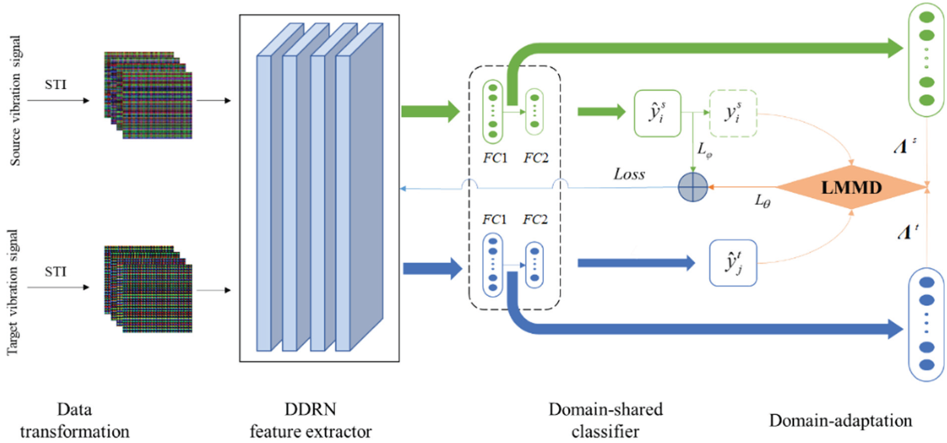
Architecture of the proposed LMMD–DDRN model.
Specifically, the output of the feature extractor DDRN is a representative vector of size 1 × 512, which is governed by the size of the input RGB image. Through a fully connected layer FC1 for dimension transformation, DDRN generates feature vectors


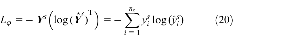
where
The target loss of the LMMD–DDRN model is defined as the sum of the domain-shared classifier loss L φ and the domain distribution disparity L θ

where
L θ is the subdomain distribution difference in the fault type across the domains and is expressed as
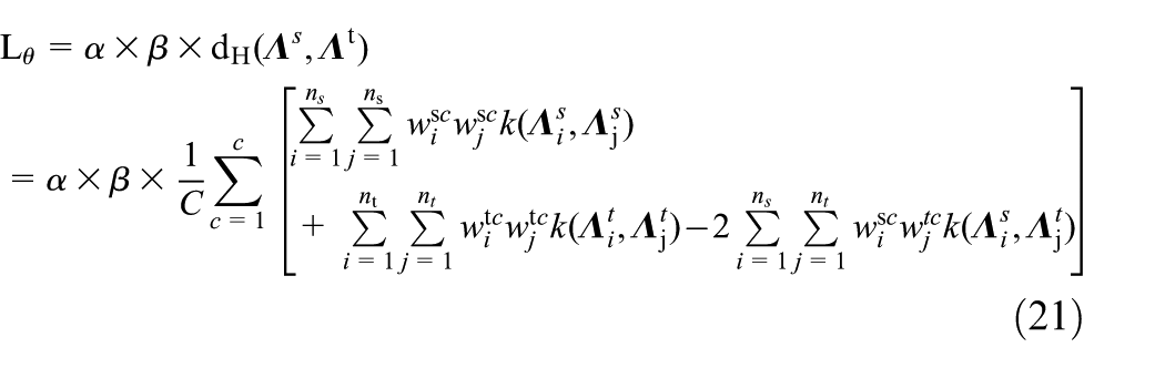
Here, dH is the LMMD, governed by equation (13). The hyperparameter α is set to 0.5, and β changes from 0 to 1 with the training epoch (Zhu et al., 2021b). Furthermore, β is defined as follows
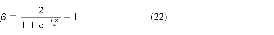
where i and N are the current epoch and the total epochs for the LMMD–DDRN model training, respectively. β tends to 0 during the early training epochs, that is, the model mainly focuses on fault classification. β approaches 1 in the latest training epochs, resulting in the considerable effect of the cross-domain distribution differences.
Experimental results and discussion
Experimental configuration
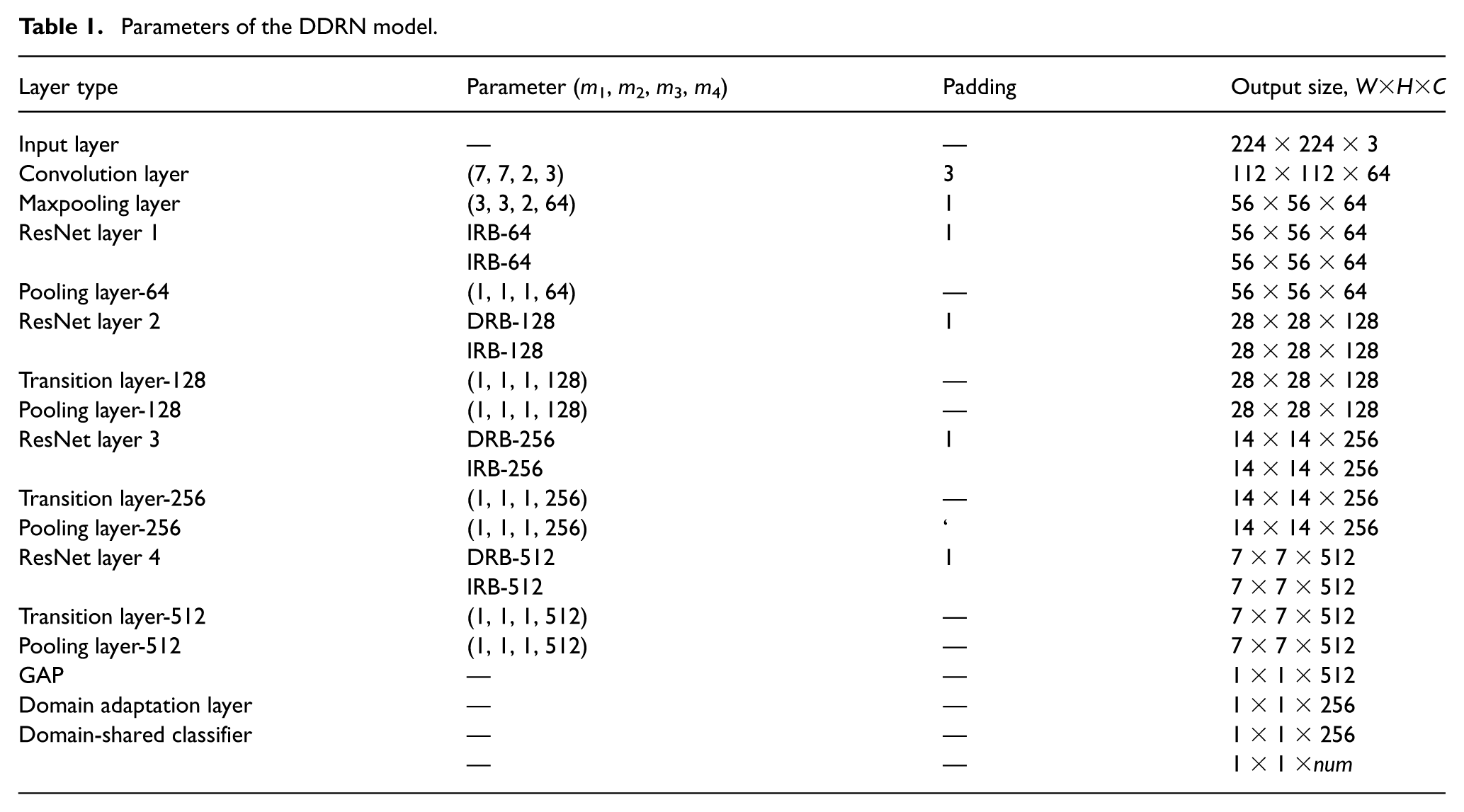
The effectiveness of the proposed diagnostic model was validated on the bearing datasets from CWRU (Hendriks et al., 2022) and Paderborn (Lessmeier et al., 2016). Experiments were conducted on a Windows system with an integrated development environment. The network model was written in Pycharm framework using Python 3.7, torch1.3.1, and torchvision 0.4.2. The parameter settings of the DDRN model are shown in Table 1. The parameter (m1, m2, m3, m4) indicates that the size of the incoming convolution kernel is m1×m2, the step size is m3, and the number of channels is m4. The parameter n in DRB-n and IRB-n corresponds to the number of convolution kernels in down-sampling residual block and identity residual block, respectively. The output size parameters W, H, and C represent the length, width, and number of channels for the feature map output, respectively. The parameter num indicates the final classification number of the network.
Parameters of the DDRN model.
In order to fully leverage the advantages of CNNs in image feature extraction, while avoiding the subjectivity and information loss introduced by parameter selection in traditional time-frequency analysis methods, this paper employs the Signal Transform Image (STI) method (Xu et al., 2023) to preprocess the original one-dimensional vibration signals. This method constructs a three-channel RGB image directly by performing segmentation and difference operations on the vibration signal, which can completely preserve the temporal dependencies and the intrinsic structure of the original signal without the need for frequency-domain transformation. The specific conversion steps of the STI method are as follows
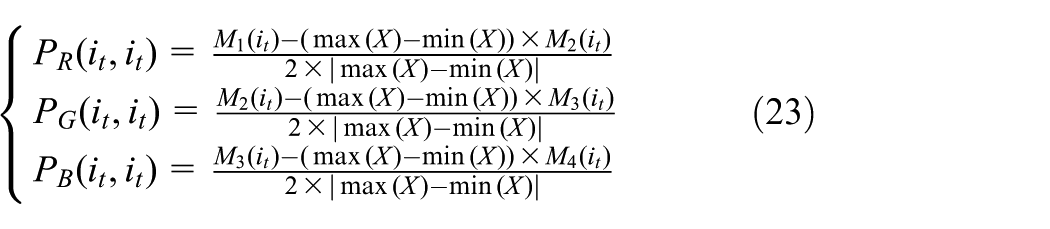
where
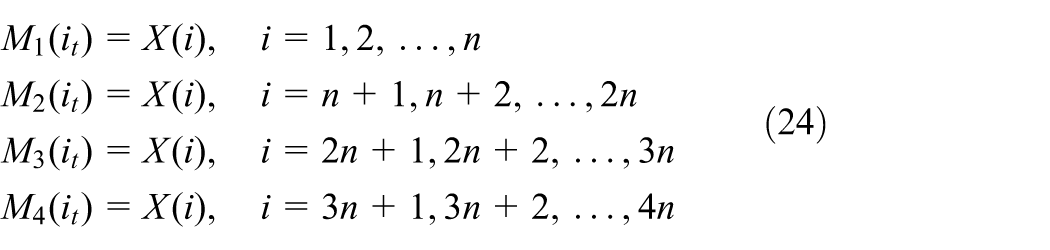
where i t = 1, 2, …, n denotes the i t -th element in the subsegment, and j = 1, 2, 3, 4 is used to index the different subsegments Mj. Through the above transformation, the original one-dimensional signal is mapped into an RGB image of size n × n × 3, where each pixel in the image corresponds to the difference result of signal points within different time windows. From a diagnostic perspective, the R channel encodes the variation relationship between the first two time windows (M1 and M2), reflecting the early evolutionary characteristics of the vibration signal; the G channel corresponds to the difference between the middle two windows (M2 and M3), capturing the dynamic characteristics of the signal in the middle stage; and the B channel is formed by the difference between the last two windows (M3 and M4), representing the attenuation or distortion information of the signal in the later stage. This channel division encodes the evolutionary information of the vibration signal at different time stages into distinct color channels, providing input features with clear physical meaning for the subsequent DL model.
Diagnosis results on the CWRU dataset
The data-acquisition test platform for the CWRU dataset recorded vibration data at different loads by installing faulty bearings in the test motor and acceleration sensors (Hendriks et al., 2022). The bearings had four types of states, that is, normal, inner race fault (IF), ball fault, and outer race fault (OF). Three directional OFs were included, that is, the 3-, 6-, and 12-o’clock positions. The fault diameters of 0.007, 0.014, 0.021, and 0.028 inches simulate various degrees of fault. During experimental validation, the model SKF 6205-2 RS JEM bearing was selected, and vibration signals were collected at different speeds at the drive end at a sampling frequency of 12 kHz. Every working condition involves five fault types, that is, ball damage at 0.007 in. (BF007) with label 0, ball damage at 0.014 in. (BF014) with label 1, inner ring damage at 0.007 in. (IF007) with label 2, inner ring damage at 0.014 in. (IF014) with label 3, and normal bearing (Normal) with label 4. During the data-preprocessing stage, a sliding window strategy was employed to segment the raw vibration signals into fixed-length samples. The sampling length for each sample was set to L = 4 × 224 to ensure that sufficient fault-related information was retained in each sample. After segmentation, the one-dimensional vibration signals were converted into two-dimensional RGB images according to the STI data-conversion method, enabling the CNN to effectively extract spatial feature representations. In the cross-domain diagnosis experiments, 130 samples collected under the 0 HP load condition were used as the labeled source domain, while 90 samples randomly collected under the 1 HP, 2 HP, and 3 HP load conditions, respectively, served as the unlabeled target domains. In each domain adaptation task, the proposed LMMD–DDRN model was trained using labeled samples from the source domain and unlabeled samples from the target domains to reduce the discrepancy in feature distributions across domains. The experiments were divided into three groups, designated as A1, A2, and A3. In all three groups, the 0 HP data were used as the source domain data, while the 1 HP, 2 HP, and 3 HP data served as the target domain data for transfer fault diagnosis, respectively.
The DDRN model was trained by minimizing the loss function in equation (19) through the stochastic gradient descent algorithm with a momentum of 0.9 and a weight decay of 0.0005. A stepwise-attenuated learning rate was adopted to improve the learning ability of the model; the damping coefficient was chosen as
After 100 training epochs with a batch size of 16, the training of the LMMD–DDRN model and the cross-domain diagnosis were completed simultaneously. Figure 5 plots the confusion matrix of the LMMD–DDRN model for the cross-domain diagnosis in classifying the five fault types from the test samples. The diagnostic accuracy of the model, misjudgment number, and misjudgment fault type are visually demonstrated simultaneously. As shown in Figure 5(a) for the cross-domain diagnosis task from 0 HP to 1 HP, we can see that of the 450 test samples for the LMMD–DDRN model, six samples were predicted incorrectly with a diagnosis accuracy of 98.67%: one sample with label 0 was misclassified as label 1. Three samples with label 1 were misclassified as label 0 and label 3. Two samples with label 3 were misclassified as label 0. All the misjudgments occurred between different fault types, while the diagnostic accuracy remains 100% for the existence of the fault state. Similar experimental results were derived for the test samples for the other two cross-domain diagnostic tasks.
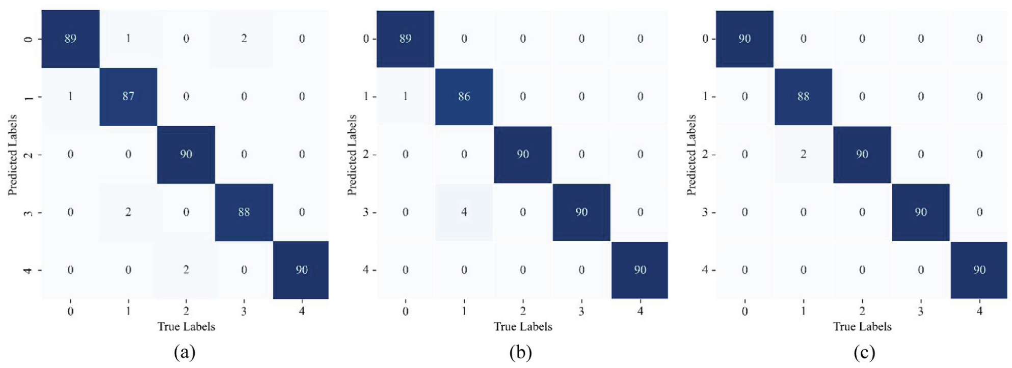
Confusion matrix of the LMMD–DDRN model on the Case Western Reserve University (CWRU) dataset: (a) A1: 0–1 HP. (b) A2: 0–2 HP. (c) A3: 0–3 HP.
For comparison, several popular transfer learning methods were employed for diagnosing the bearing fault, that is, the deep domain confusion (DDC) (Tzeng et al., 2014), modified deep adaptation networks (DANs) (Wang et al., 2015), and domain adversarial training of neural networks (DANN) (Ganin et al., 2015). As a benchmark method for comparison, ResNet networks (He et al., 2016) were also investigated. All methods adopted the same loss function, batch size, and number of iterations.
Labeled source domain samples and unlabeled target domain samples were used for model training, but only the latter were used for testing. In addition, ResNet used LMMD to regulate the cross-domain difference. Figure 6 compares the cross-domain diagnosis results of the aforementioned four models with those of the proposed LMMD–DDRN model. As shown in Figure 6, DANN and DDC models deliver poor performance owing to their shallow network structure and limited representation ability. As the load is gradually increased from 0 HP to 3 HP, the accuracy of DANN and DDC models decreases gradually, making it difficult to solve the problem of unlabeled target domain fault diagnosis effectively. The diagnosis accuracy of DAN on cross-domain tasks 0–1 HP, 0–2 HP, and 0–3 HP is 92.67%, 88.89%, and 95.11%, respectively. The ResNet model, which also uses LMMD to adjust for inter-domain differences, has a diagnosis accuracy of 98.67% and 94.89% on the cross-domain tasks 0–1 HP and 0–2 HP, respectively, but the diagnosis accuracy on the cross-domain task 0–3 HP is only 56.89%. The LMMD–DDRN model proposed in this article achieved the best classification performance in the migration tasks 0–1 HP, 0–2 HP, and 0–3 HP, with 98.67%, 98.89%, and 99.56%, respectively.
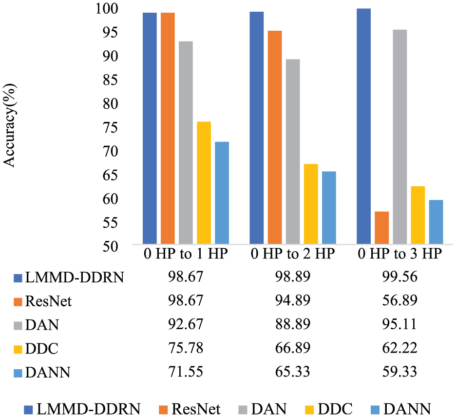
Experimental results on three cross-domain tasks using different fault diagnostic methods on the CWRU dataset.
As can be seen from the t-Distributed Stochastic Neighbor Embedding (t-SNE) visualization results, in Figure 7 significant differences exist among different models in terms of feature discriminability and cross-domain alignment capability. LMMD–DDRN achieves the best performance: samples from the source and target domains belonging to the same fault category are highly mixed, forming compact intra-class clusters with clear inter-class boundaries. This indicates that the class-conditional alignment mechanism effectively eliminates subdomain distribution shifts. ResNet can distinguish different fault categories relatively well; however, samples from the source and target domains within the same class remain clearly separated, reflecting the impact of distribution shift in the absence of domain adaptation. Both DAN and DDC alleviate domain shift to some extent through MMD-based alignment, but DDC performs slightly worse than DAN, suggesting that multi-kernel MMD provides more effective alignment than single-kernel MMD. In contrast, DANN shows the poorest performance. Although adversarial training attempts to confuse domain representations, it leads to blurred class boundaries, with some categories becoming mixed. As a result, the source and target domains fail to align properly, producing a chaotic overall feature distribution. In summary, LMMD–DDRN achieves the best cross-domain feature alignment while preserving clear class separability, thereby demonstrating the superiority of the proposed method.
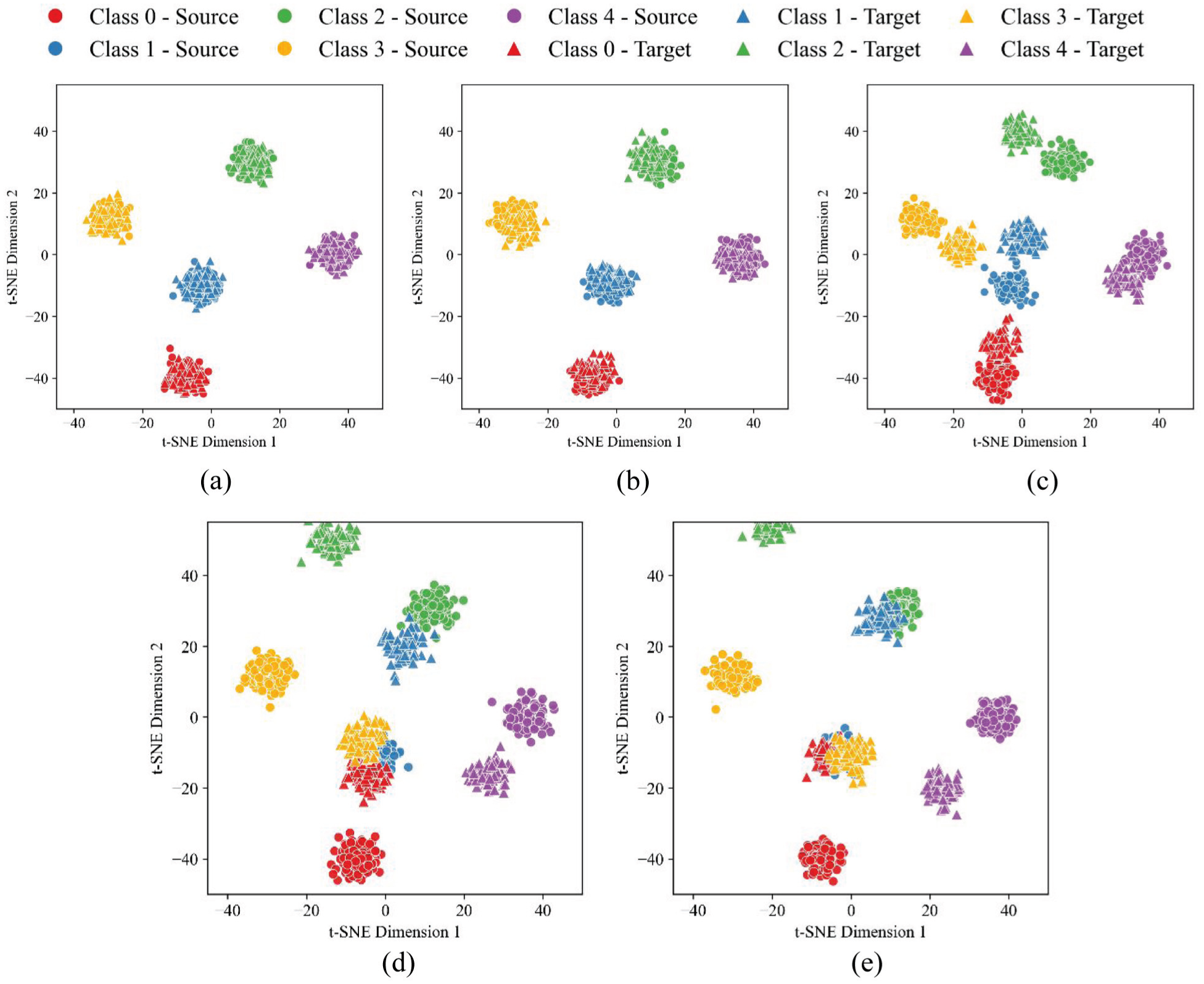
Visualization results of the CWRU dataset: (a) LMMD–DDRN. (b) ResNet. (c) DAN. (d) DDC. (e) DANN.
Diagnosis results on the Paderborn dataset
The data-acquisition test bench of the Paderborn dataset mainly comprises an electric motor, a torque-measurement shaft, a bearing test module, a flywheel, and a load motor (Lessmeier et al., 2016). Appropriately selecting the applied load torque [N·m], rotational speed of the motor [r/min], and radial force [N] ensured that the bearing operation involved four states: S0 with a load torque of 0.7 N·m, a radial force of 1000 N, and a motor speed of 1500 r/min; S1 with a load torque of 0.1 N·m, a radial force of 1000 N, and a motor speed of 1500 r/min; S2 with a load torque of 0.7 N·m, a radial force of 400 N, and a motor speed of 1500 r/min; S3 with a load torque of 0.7 N·m, a radial force of 1000 N, and a motor speed of 900 r/min. During the experimental validation, the bearing fault data were sampled at a rate of 64 kHz and contained three types of faults, that is, the inner ring fault (IRF), the OF, and the fault-absent bearing (Normal). Similar to the CWRU experiments, the raw vibration signals from the Paderborn dataset were segmented into fixed-length samples using a sliding-window approach. Each sample segment was then converted into an RGB image representation as the input for the DL model. A total of 130 samples from the S0 condition were selected as the labeled source domain dataset, while 90 samples from each of the S1, S2, and S3 conditions were used as the unlabeled target domain datasets. Four sets of experiments were designed: the transfer diagnosis tasks from the source domain to each of the other three datasets were defined as B1, B2, and B3, respectively. The samples from the target domains were used for domain adaptation during the model training to minimize the differences in distributions across the domains.
Figure 8 plots the confusion matrix of the LMMD–DDRN model in classifying cross-domain fault types on the test samples. As shown in Figure 8(a) for the cross-domain diagnosis task B1, the LMMD–DDRN model correctly predicted all test samples; for cross-domain tasks B2 and B3, 8 and 11 samples were misclassified, respectively.
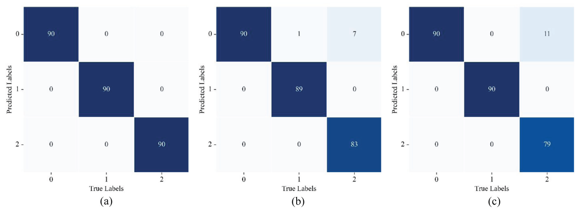
Confusion matrix of the LMMD–DDRN model on the Paderborn dataset: (a) B1. (b) B2. (c) B3.
Moreover, Figure 9 compares the cross-domain diagnostic performance of the LMMD–DDRN model with other models on the Paderborn dataset. Similar to the results on the CWRU dataset, the LMMD–DDRN model achieved the best classification accuracy of 100%, 97.04%, and 95.93% for tasks B1, B2, and B3, respectively, on the Paderborn dataset.
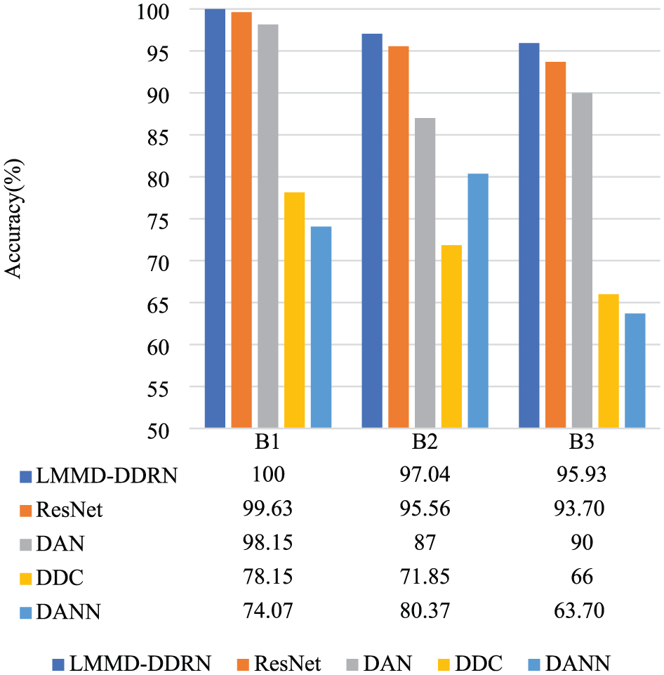
Experimental results for three cross-domain tasks using different fault diagnostic methods on the Paderborn dataset.
The t-SNE visualization results on the Paderborn dataset are highly consistent with the observations from the CWRU dataset. LMMD–DDRN still achieves the best cross-domain feature alignment, where samples from the source and target domains belonging to the same fault category are closely mixed, and the inter-class boundaries remain clear. Although ResNet can distinguish different fault types, samples from the same class but different domains remain clearly separated, indicating the influence of domain shift without adaptation. DAN and DDC partially alleviate the domain shift through MMD-based alignment, with DAN performing slightly better than DDC. In contrast, DANN shows the worst performance, where adversarial training leads to blurred class boundaries and mixed samples across categories. These results further demonstrate the generalization ability and robustness of LMMD–DDRN under different operating conditions.
Comparison with non-graph deep models
To conduct a more comprehensive evaluation of the proposed framework, the two-dimensional convolution layers in LMMD–DDRN were replaced with a one-dimensional convolution. Several widely used non-graph DL models were introduced for comparison, including a one-dimensional convolutional neural network (1D-CNN) (He et al., 2021), which captures shallow temporal patterns and partial frequency-domain features from time-series data through local receptive fields, suitable for handling short-term dependencies in vibration signals; a Long Short-Term Memory network (LSTM) (Chen et al., 2025), which alleviates the vanishing gradient problem effectively through gating mechanisms and models long-term temporal dependencies, demonstrating excellent performance when processing vibration signals with long-range dependencies; and a Transformer encoder (Zhang et al., 2023), which models correlations between arbitrary positions in sequences based on the self-attention mechanism, capable of capturing global information and excelling in capturing complex long-range dependencies. These methods were widely applied in time-series analysis and fault diagnosis tasks. Their performance was evaluated under the same sample size, training epochs, optimizer, and other training conditions to objectively assess the robustness of LMMD–DDRN when handling one-dimensional data.
As shown in Figure 10, the 1D LMMD–DDRN model significantly outperforms the above models in all cross-domain tasks, particularly in the 0 HP to 3 HP task, where the accuracy reached 86.89%, nearly 50% higher than that of LSTM and Transformer. This phenomenon suggests that traditional sequential models face significant disadvantages when dealing with complex cross-domain distribution shifts, as their learned parameters heavily depend on the specific distribution of the training data, leading to performance degradation after transfer. Both LSTM and Transformer are more reliant on global temporal dependencies or attention patterns, which tend to fail under changing operational conditions (Zhu et al., 2023). In contrast, 1D-CNN performs significantly better than LSTM and Transformer, which is related to its ability to effectively capture local effects and periodic patterns in the vibration signal (He et al., 2021; Huo et al., 2022). However, due to the lack of domain adaptation mechanisms, the overall performance of 1D-CNN is still lower than that of LMMD–DDRN, further validating the effectiveness of the class-conditional alignment strategy in this study for one-dimensional tasks.
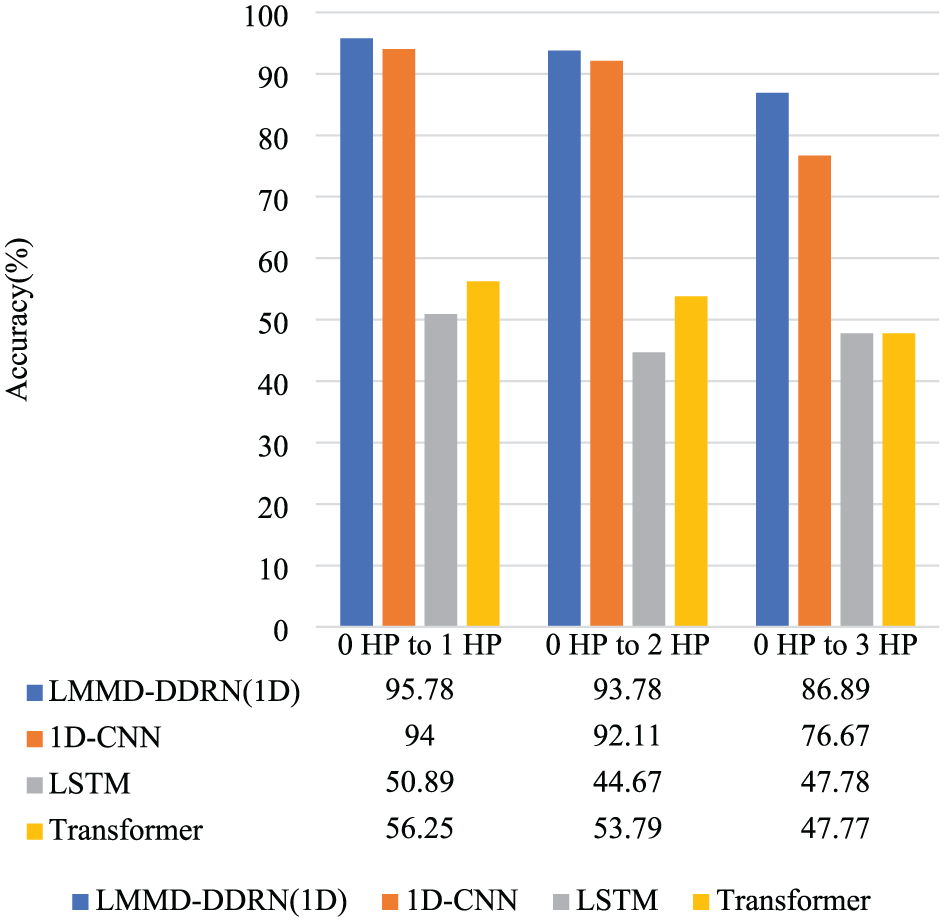
The results of three cross-domain tasks on the 1D CWRU dataset.
The results in Figure 6 suggest that models based on 2D image inputs generally outperform those based on 1D inputs, as 2D data provides multi-scale features that facilitate convolution operations and supply robust feature spaces for domain adaptation algorithms, offering better cross-domain performance, despite the increased computational cost.
As shown in Figure 11, the LMMD–DDRN model significantly outperforms 1D-CNN, LSTM, and Transformer on the Paderborn dataset. The latter three models did not specifically address the distribution differences of similar fault samples in the cross-domain scenario, leading to noticeable degradation during transfer. In contrast, LMMD–DDRN explicitly minimizes the intra-class differences between the source and target domains through its class-conditional alignment mechanism, effectively mitigating class confusion. These results fully validate the effectiveness of the proposed strategy in handling cross-domain diagnostic tasks.
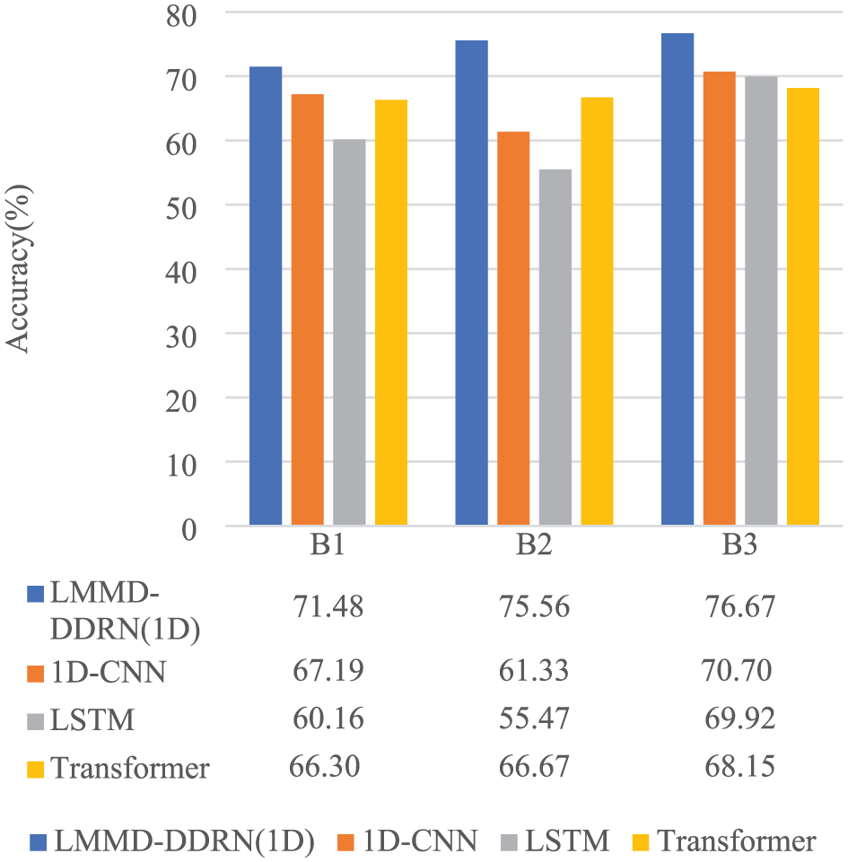
The results of three cross-domain tasks on the 1D Paderborn dataset.
On the other hand, as shown in Figure 12, the performance of LMMD–DDRN with 2D input still outperforms that of 1D input, which is consistent with the results on the CWRU dataset. This further confirms that 2D convolution networks provide richer and more robust multi-scale feature spaces, thus improving cross-domain alignment.
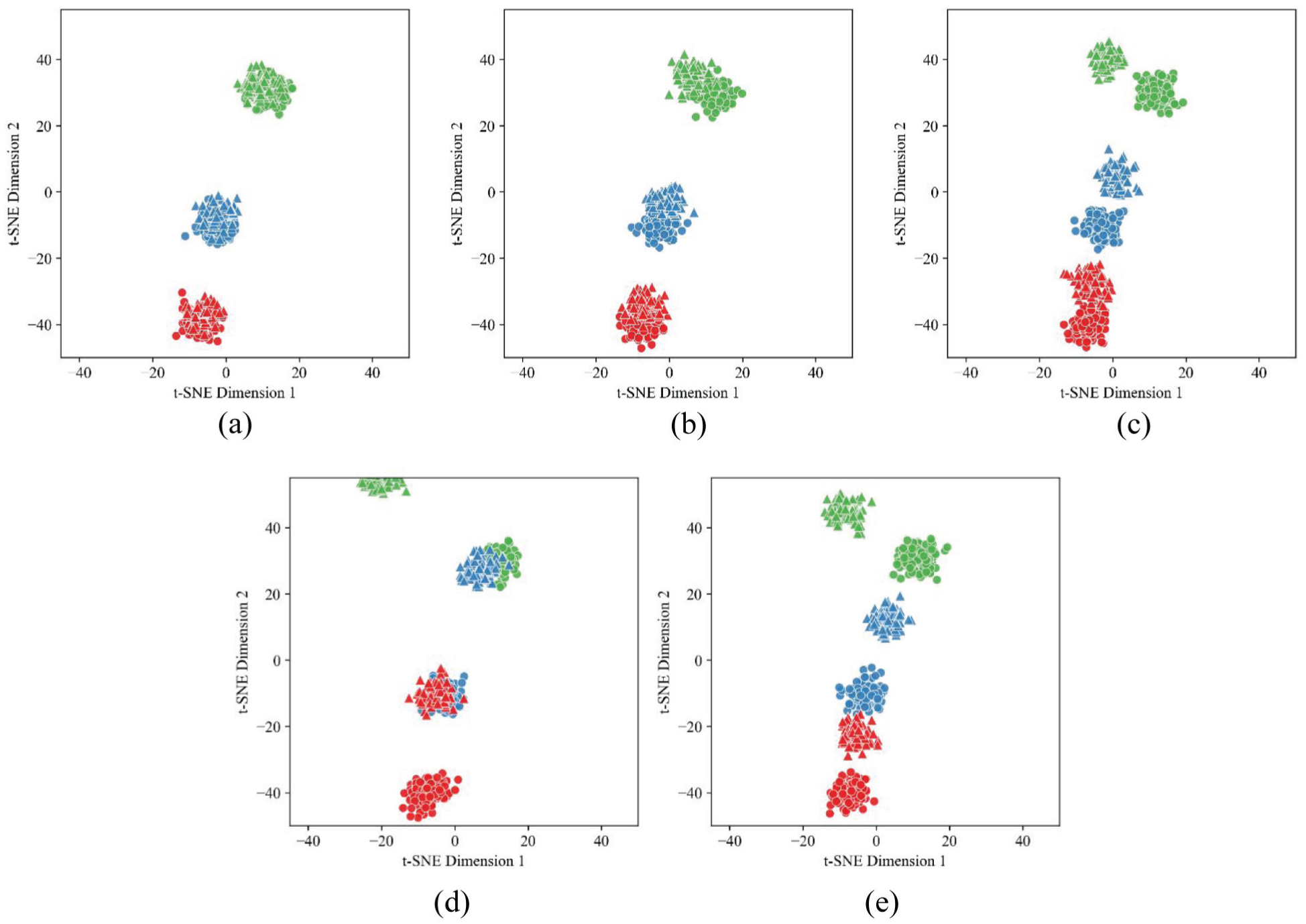
Visualization results of the Paderborn dataset: (a) LMMD–DDRN. (b) ResNet. (c) DAN. (d) DDC. (e) DANN.
Ablation studies on LMMD and DDRN
To clarify the role of each component, ablation experiments were designed for the LMMD alignment module and the DDRN backbone. Four model variants were included in the experiments: standard ResNet, LMMD–ResNet, DDRN, and the complete LMMD–DDRN. Performance differences between these variants reveal the specific contributions of class-conditional alignment and dense residual connections. Through this comparison, the complementary effect of LMMD and DDRN is highlighted, and their combination is shown to be essential for achieving robust cross-domain fault diagnosis.
As shown in Figure 13, after introducing the LMMD loss for domain adaptation, both DDRN-based and ResNet-based models achieved significant improvements in diagnosis performance across all three cross-domain tasks. Notably, in the 0–3 HP task, LMMD–ResNet improved accuracy by approximately 28.89% compared with the ResNet, and LMMD–DDRN improved accuracy by approximately 28.23% compared with DDRN. This enhancement was primarily attributed to the LMMD module’s ability to explicitly minimize subdomain distribution differences between source and target domains in the feature space, thereby effectively mitigating classification degradation caused by domain shifts. It is worth noting that LMMD–DDRN consistently outperformed LMMD–ResNet across all cross-domain tasks, indicating that DDRN’s strengthened global feature-extraction capability via dense connections provides more discriminative feature representations for LMMD, further enhancing the model’s generalization capacity.
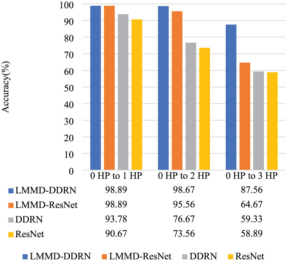
The ablation experiment results on the CWRU dataset.
As shown in Figure 14, similar patterns were observed on the Paderborn dataset: LMMD–DDRN and LMMD–ResNet significantly outperformed their respective base models, DDRN and ResNet, reaffirming the LMMD module’s effectiveness. In particular, for identifying complex faults such as B3, LMMD–DDRN exhibited a notable advantage over LMMD–ResNet, further demonstrating that DDRN’s ability to capture rich global information through dense connections is a key component in building high-performance cross-domain diagnostic models.

The ablation experiment results on Paderborn dataset.
Testing on the noisy data
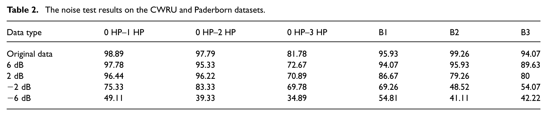
In the first phase of the study, the effectiveness of the LMMD–DDRN framework in addressing the core issue of “domain shift” was verified using relatively ideal data conditions to control variables and ensure clarity of conclusions, without considering the influence of real-world factors. In practical applications, environmental or mechanical noise often significantly degrades the accuracy and reliability of diagnostic models. To further evaluate the model’s performance on noisy data and validate its high reliability for real applications, Gaussian white noise with different Signal-to-Noise Ratio (SNR) levels was added to the CWRU and Paderborn target domain datasets, and preliminary noise testing experiments on the LMMD–DDRN model were conducted. The experimental results are shown below.
As seen from the results in Table 2, when noise is mild (e.g., experiments with 6 dB and 2 dB), LMMD–DDRN’s accuracy remains relatively high, indicating a certain degree of robustness of the model. However, when the noise intensity increases to −6 dB, LMMD–DDRN’s performance significantly drops. For instance, in the B2 task on the Paderborn dataset, accuracy decreases from 99.26% to 41.11%, representing a reduction of about 58 percentage points, with some tasks even falling below 40%. This indicates that under low SNR conditions, the performance of LMMD–DDRN on cross-domain diagnostic tasks degrades substantially due to noise.
The noise test results on the CWRU and Paderborn datasets.
Computational efficiency and deployment feasibility analysis
To further assess the usability of LMMD–DDRN in real industrial scenarios, the model’s parameter scale, computational complexity, and inference speed were calculated. The experiments were conducted on an Ubuntu 20.04 system, equipped with an Intel i7-11700K CPU and an NVIDIA GeForce RTX 3080 Ti GPU. The experimental results are shown in Table 3.
The calculation results of the evaluation parameters of LMMD–DDRN.
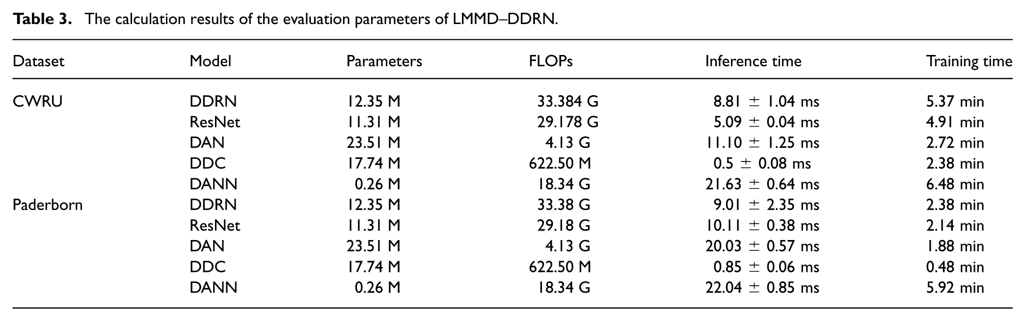
As seen from the results, LMMD–DDRN has approximately 12.35 million parameters, which is lower than those of the DAN and DDC models but slightly higher than that of ResNet. This indicates that, while maintaining feature-extraction capability, LMMD–DDRN achieves better deployment feasibility. Its computational complexity is around 33.384 GFLOPs, similar to that of the ResNet model, and the addition of the class-conditional alignment module has not significantly increased the parameter burden. Moreover, the average inference time for LMMD–DDRN on the CWRU and Paderborn datasets is 8.81 ms and 9.01 ms, respectively, which corresponds to an effective diagnostic frequency of about 110–115 Hz, higher than the typical 10–100 Hz frequency of industrial rotating machinery. In comparison, DDC, although faster in inference, suffers from lower cross-domain diagnostic performance, and DANN and DAN exhibit significantly higher inference delays. The total training time for LMMD–DDRN on both datasets is 5.37 min and 2.38 min, respectively, similar to that for ResNet, and much lower than that for DANN, indicating that the LMMD alignment mechanism does not introduce excessive training overhead.
Conclusion
Cross-domain bearing fault diagnosis remains a challenging problem due to domain drift caused by varying operating conditions, which leads to distribution discrepancies between source and target domains. Conventional domain adaptation methods usually perform global distribution alignment, which may inadvertently mix features from different fault classes and cause inter-class confusion, thereby degrading diagnostic performance. To solve this problem, an improved ResNet diagnostic model with a domain adaptation mechanism was proposed. A dense connection structure was introduced between the residual blocks in ResNet, that is, DDRN (Xu et al., 2023). This model realized robust feature extraction even with limited feature information under various operating conditions and provided sufficient transferable features from the source and target domains to avoid the overfitting of deep networks (Huang et al., 2017). Subsequently, the domain adaptation mechanism used the LMMD to evaluate domain drift. Through feature-distribution alignment of the same fault class in the relevant subdomains, feature differences across the source and target domains were minimized to guarantee the cross-domain prediction accuracy of the diagnostic model. The experimental validation results on the CWRU and Paderborn datasets demonstrated the superiority of the proposed model over the popular transfer learning methods.
However, it must be noted that the experimental evaluation in this study was conducted under relatively ideal conditions (i.e., clean, well-structured benchmark datasets), which, while beneficial for clearly validating the core algorithm’s effectiveness, also represents a limitation of this present work. Industrial environments are often characterized by noise, missing data, and multi-source data complexities. Therefore, future research will focus on enhancing the model’s robustness and generalization in more challenging scenarios, with specific plans as follows. (1) Noise robustness validation: A systematic study on model performance under various noise types, including Gaussian white noise, impulse noise, and varying SNR conditions, will be carried out. The impact mechanisms of noise on feature extractors and domain-alignment modules will be analyzed, and the feasibility of integrating noise-resistant modules or designing robust loss functions will be explored. (2) Multi-modal information fusion: The expansion of the model framework to handle multi-source heterogeneous sensor data will be explored. The core idea is to design a multi-stream network (Zhao et al., 2025) architecture to extract modality-specific features and develop cross-modal domain-alignment strategies, aiming to leverage multi-modal information for more robust cross-domain diagnosis. (3) Few-shot and class-imbalanced learning: To address the few-shot problem, we plan to introduce meta-learning strategies (Stergiadis et al., 2021), such as Model-Agnostic Meta-Learning (MAML), into the model. This will improve its ability to quickly adapt to new categories with few-shot samples. In addition, data-augmentation methods like Generative Adversarial Network (GAN) (Robb et al., 2020) will be used to augment minority class samples. To tackle class imbalance, weighted loss functions (Wei et al., 2023) will be incorporated during model training to focus on the minority classes, and resampling techniques will be employed to balance the dataset.
In summary, the LMMD–DDRN framework proposed in this study provides an effective solution to the domain-shift problem in intelligent fault diagnosis, and overcoming the aforementioned practical challenges will be key to moving from theoretical validation to industrial application.
Footnotes
Funding
The authors disclosed receipt of the following financial support for the research, authorship, and/or publication of this article: This work was supported by Scientific and Technological Research Projects in Henan Province, 232102210092, and Key Research Projects of Higher Education Institutions in Henan Province, 25A120004.
Declaration of conflicting interests
The authors declared no potential conflicts of interest with respect to the research, authorship, and/or publication of this article.
Data availability statement
The CWRU dataset is accessible at https://csegroups.case.edu/bearingdatacenter/pages/welcome-case-western-reserve-university-bearing-data-center-website. The Paderborn dataset is accessible at ![]()