
Abstract
This study addresses the analyses of the ultra-low frequency oscillation of active power in hydroelectric plant caused by flow factors in the tailrace channel. We focus on mathematically describing the hydraulic dynamic characteristics of the pipe and channel mixed flows in the tailrace system. First, a discrete frequency-domain equivalent circuit model is proposed. Based on the circuit equivalence principle, this model derives the transfer matrix for a complex hydraulic system consisting of pressurized pipelines, open channels, and branch channel junctions. Based on the proposed model, a novel stability evaluation strategy for the complicated hydraulic system is developed. By judging the oscillation order and then identifying the corresponding dominant eigen mode, the critical stability boundary of the observed ultra-low-frequency oscillation can be accurately determined by tracking the exact oscillation mode, thus avoiding searching for all the eigenvalues of the system that correspond to all oscillation orders. This scheme compensates for the limitations of the existing continuous frequency-domain model in the stability analysis of specific natural frequency orders. By comparing the critical stability turning points of ultra-low frequency oscillation obtained from field measurement data with those from simulation analysis, the model’s capability to accurately evaluate the stability of multi-unit hydropower systems under various operating conditions is validated.
Keywords
Introduction
With the large-scale integration of hydropower, wind power, and photovoltaic power into regional interconnected power grids, the stability of power systems has been increasingly affected by low-frequency and ultra-low-frequency oscillations (Wang et al., 2019. 2020). Flow and head fluctuations widely exist in the pipeline systems of hydropower stations, and such fluctuations become more complex and difficult to control in composite hydraulic systems consisting of pressurized pipelines and open channels. As a transitional flow regime between pressurized flow and open-channel flow, free-surface-pressurized flow combines the pressure constraint effect of pressurized flow and the free-surface fluctuation characteristics of open-channel flow. Its flow state is prone to abrupt changes under the coupled influence of multiple factors such as discharge, pipe diameter, and slope, making it the most nonlinear and uncertain flow pattern in hydraulic systems (Teng et al., 2025; Wylie and Streeter, 1993). These sustained oscillations not only threaten the safe and stable operation of the system and reduce the power generation efficiency of hydroelectric units, but also induce severe safety hazards such as pipeline fatigue damage and abnormal vibration of units (Shi et al., 2023; Yang, 2018). Therefore, conducting research on the hydraulic characteristics of free-surface-pressurized flow and revealing its flow laws and oscillation mechanisms is of great significance for ensuring the safe and efficient operation of composite hydraulic systems in hydropower stations.
At present, scholars have carried out extensive and cutting-edge research in the fields of complex pipeline modeling and system stability analysis. In the study of open-channel flow and free-surface-pressurized flow, Cheng et al. (2007) established a numerical solution method for the free-surface-pressurized flow transition process based on hydrodynamic equations, revealing the evolution law of free-surface-pressurized flow under sudden discharge changes. In the coupled modeling of complex pipe networks, the Australian Lambert team combined graph theory and the state-space method to propose a transient analysis model suitable for multi-branch and multi-condition pipe networks, promoting the refined modeling of complex pipeline systems (Zeng et al., 2022a). Nevertheless, existing international research still has limitations. For complex pipeline systems with coupled pipe flow and open-channel flow, there is a lack of frequency-domain modeling methods that balance computational efficiency and accuracy. The research on the ultra-low-frequency oscillation mechanism induced by free-surface-pressurized flow is insufficient, which can hardly meet the stability analysis requirements of complex hydraulic systems in large-scale hydropower stations (Zeng et al., 2022b).
In terms of frequency-domain modeling methods, the traditional hydraulic impedance method and the continuous transfer matrix method have been widely used in hydraulic oscillation analysis (Alubokin et al., 2022; Chaudhry, 2014; Kan et al., 2021a; Vítkovsky et al., 2011). However, the former is difficult to adapt to complex pipe networks with branches and free-surface-pressurized flow (Guo and Zhu, 2021; Liu et al., 2022; Yang et al., 2018), and the latter is prone to errors in modal analysis of specific orders (Chen et al., 2021; Suo and Wylie, 1989; Yan et al., 2014). To solve the modeling problem of distributed parameter systems, the equivalent circuit method (ECM) has gradually become the mainstream due to its advantages in hydraulic-electric analogy (Jaeger, 1977; Kan et al., 2021b; Paynter, 1953). Foreign scholars analogized the water hammer fluctuation in pressurized pipelines to the electromagnetic propagation in transmission lines and established a discrete impedance model, which significantly improved the adaptability of frequency-domain modeling for complex pipe networks (Nicolet, 2007). Zhao et al. (2019) applied the equivalent circuit method to dynamically analyze the operating condition conversion process of pumped storage power stations and achieved satisfactory results. Zheng et al. (2023) proposed a hybrid modeling approach combining the continuous transfer matrix and circuit equivalence for the free-surface-pressurized flow tailwater system of hydropower stations, realizing the global stability analysis of full-order natural frequencies. However, there is still a lack of accurate and targeted solution for ultra-low-frequency dominant oscillation modes.
Regarding the mechanism of ultra-low-frequency oscillations and stability criteria, existing studies mostly focus on the negative damping of turbine governing systems, power grid damping characteristics, and time-domain simulation verification. The stability boundary of the system is generally obtained through full-mode scanning, which involves a large amount of computation and is easily disturbed by non-dominant frequencies (Wang et al., 2024). Recent studies have shown that the field ultra-low-frequency oscillations in hydropower stations are usually dominated by a certain dominant hydraulic mode (Shi et al., 2025; Zheng et al., 2022). However, how to accurately match this mode using measured data and realize efficient stability determination only by tracking the eigenvalues of the system mathematical model for specific orders remains a difficult problem in engineering and theory.
Based on this foundation, this paper proposes a frequency-domain discrete circuit equivalence model specifically for the stability issue caused by the ultra-low frequency oscillations in complex hydropower station systems. First, determine the corresponding ultra-low frequency oscillation order and then judge the stability of the system based on this order. Using the tailrace system of a large hydropower plant in Southwest China as a case study, this paper develops a model. The critical stability power predicted by the simulation was benchmarked against the plant’s field measurements, and the close agreement validates the effectiveness of the proposed modeling approach.
The main innovative points of this article are as follows:
A circuit equivalence method for frequency-domain system modeling is proposed, which exhibits satisfactory adaptability in the modeling of complex pipeline systems that contains pipe and channel flows.
The system matrix is solved to obtain solutions of all orders corresponding to different power levels. The oscillation order is first determined from field measurements, and the corresponding dominant eigenmode is then identified. The critical stability boundary of the observed ultra-low-frequency oscillation can be accurately determined by tracking only this specific oscillation mode, thereby avoiding the need to search all eigenvalues of the system associated with all oscillation orders. This targeted strategy eliminates the interference of irrelevant frequency components and improves the stability analysis precision of the hydropower plant.
System modeling
Background information of the system plant
The station adopts a typical one-tunnel for two-turbine layout, which is commonly used in the construction of multi-unit flow passages in modern large hydropower stations. The system schematic is shown in Figure 1, with key structural parameters indicated in the plot. It is denoted that the tailrace flow is not entirely in the pressurized state. The tailrace extension is a pressurized pipeline, and the main tailrace tunnel and branch tunnels are open channels. For detailed system parameters, please refer to Appendix 2.
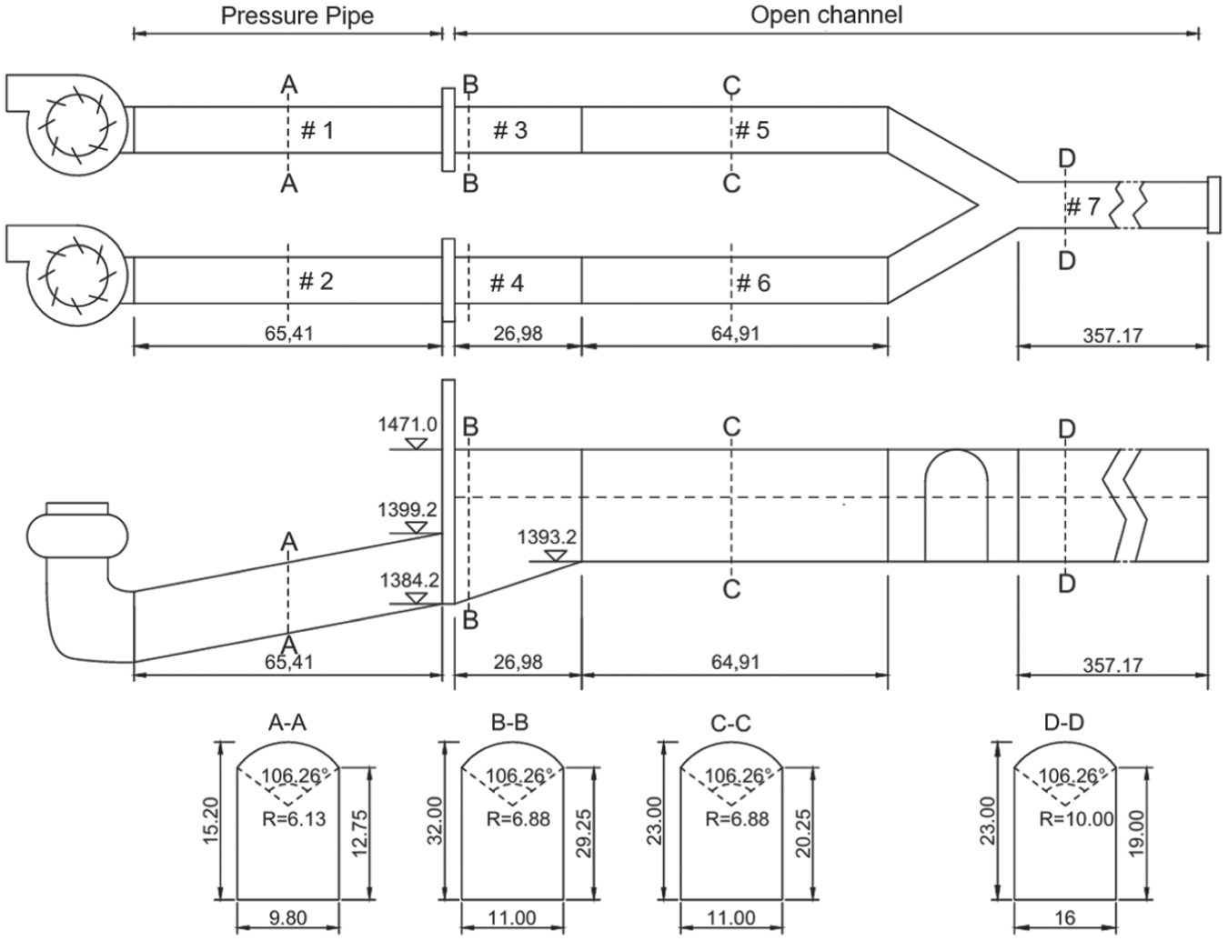
Tailrace system diagram.
Engineering practice shows that the unit will experience ultra-low-frequency power oscillations with a cycle of approximately 16 seconds within a wide operating range, corresponding to a frequency of 0.0625 Hz (ω≈0.3926 rad/s), and water depth fluctuations of the same period were measured simultaneously in the two tailrace gate chambers.
Through on-site tests, no abnormal vibrations or pressure pulsations were observed in the upstream pipeline during unit power oscillations, so the upstream excitation source can be excluded. The turbine manufacturer verified that no obvious cavitating vortex occurred, and no abnormal mechanical or electromagnetic vibrations were detected. These results indicate that non-hydraulic factors of the turbine are not directly related to the hydraulic oscillation. Other non-hydraulic factors, such as the turbine governor, generator exciter, and Power System Stabilizer (PSS), have also been eliminated in field tests. Experts from the power plant, manufacturer, and design institute confirmed that such power oscillations are caused by hydraulic imbalance in the tailrace system under specific operating conditions. Therefore, the modeling work focuses on the tailrace system to achieve a reasonable simplification of the overall system.
Networked transfer matrix of hydraulic components
Equivalent model of pressure pipe and open channel
The transfer matrix can be divided into field transfer matrix and point transfer matrix, representing the hydraulic state relationship at both ends of the pipeline and the transfer characteristics at a certain boundary, respectively (Chaudhry, 2014). The modeling of pressure pipelines and open channels belongs to the field transfer matrix, while the modeling of connection of turbines, pipe connections, confluence outlets, and tailrace outlets is the point transfer matrix (Vítkovsky et al., 2011).
The hydraulic dynamic characteristics of pressurized pipes with any cross-sectional shape can be formulated as the partial differential equation system Saint-Venant equation in equation (1) (Vítkovsky et al., 2011)
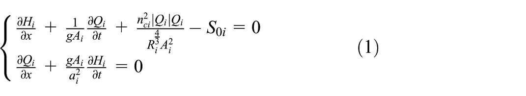
where
Equation (1) can be linearized near the steady-state points
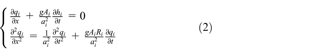
where
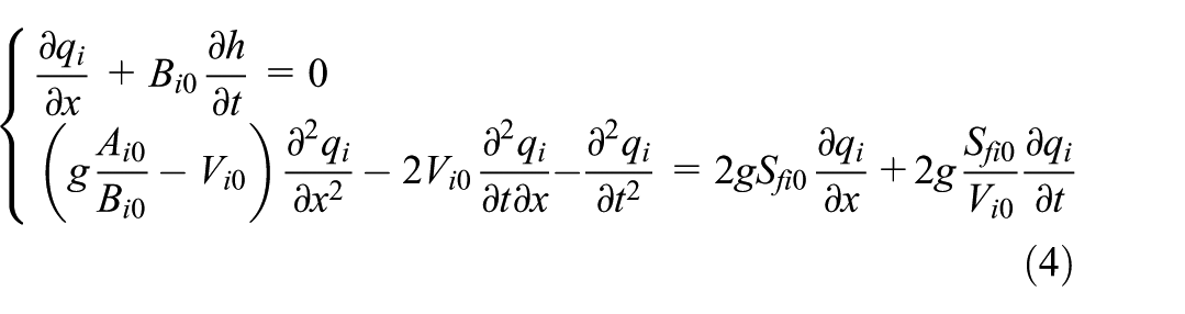
Similarly, from the continuity equation and momentum equation of the open channel, the hydraulic dynamic characteristics of the horseshoe-shaped open channel can be deduced as shown in equation (3) (Vítkovsky et al., 2011)
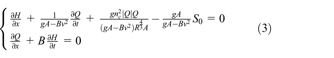
where B represents the width of the water surface; v represents the flow velocity; H represents the water depth inside the open channel.
Equation (3) can be linearized near the steady-state points
where
With voltage U and current I as variables, the propagation law of electromagnetic waves in the conductor conforms to the telegraph equation (Zheng et al., 2021), and the specific expression is
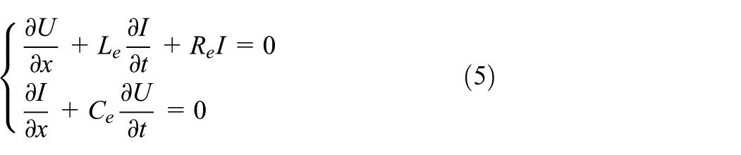
where
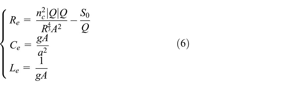
Therefore, if H and Q are used to replace U and I in the circuit, the hydraulic dynamic characteristic equations of the pressurized pipe and the open channel will have the same structural form as the telegraph equation (5). Hence, the circuit model can be extended to the modeling of the hydraulic dynamic characteristics of pipes (channels), and the equivalent resistance, inductance, and capacitance mathematical formulas of the circuit equivalent models of pressurized pipes and open channels can be obtained from equations (1) and (3).
The pressurized pipe equivalent circuit parameters are represented as shown in equation (6)
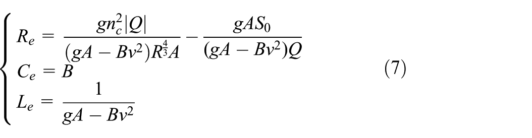
The open channel equivalent circuit parameters are represented as shown in equation (7)
The system of ordinary differential equations can be directly derived from Kirchhoff’s law to obtain equation (8)
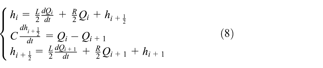
Combined with equation (8), the transfer matrix of the equivalent circuit is obtained
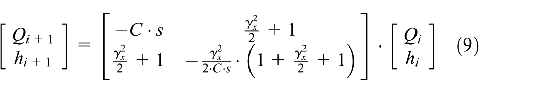
In the formula,
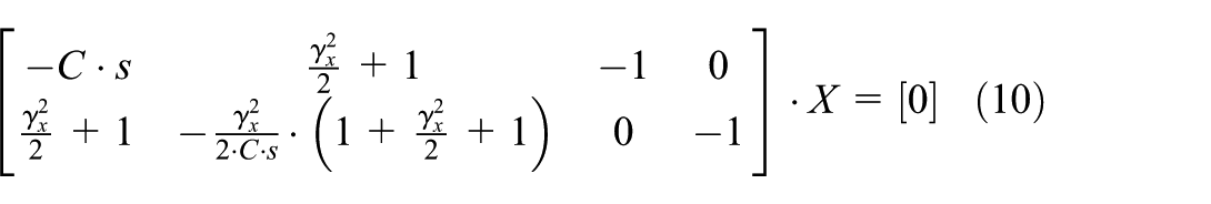
The field matrix blocks of the pressure pipe and open channel can be transformed by equation (9), as shown in equation (10)
Modeling of hydraulic boundaries
Boundary conditions of the turbine
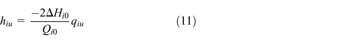
In this paper, two water turbines are regarded as the upstream boundaries of the tailrace system. Given that this study only focuses on the non-constant water depth fluctuations in the tailrace under specific guide vane opening and governor withdrawal conditions, it is reasonable to simplify the unit to a fixed orifice based on hydraulic theory. Thus, the flow and head deviations are related as in equation (11)
where
Applying equation (11) to the outlet-boundary point-matrix blocks of the two turbines yields equations (12) and (13), respectively

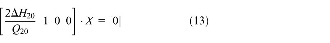
In the transfer matrix of system, the entries associated with the i th turbine’s point transfer matrix are found in row (
Boundary treatments at the connection points of pipes and channels
From the energy conservation equation at the connection of pipes or channels (considering local hydraulic losses), it can be concluded that
where the i th and j th pipes (channels), respectively, represent the pipes before and after the connection.
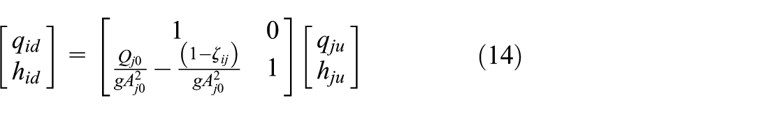
The sub-matrix blocks linked by pressure pipes and open channels are transformed via equation (14), with the outcome given in equation (15)
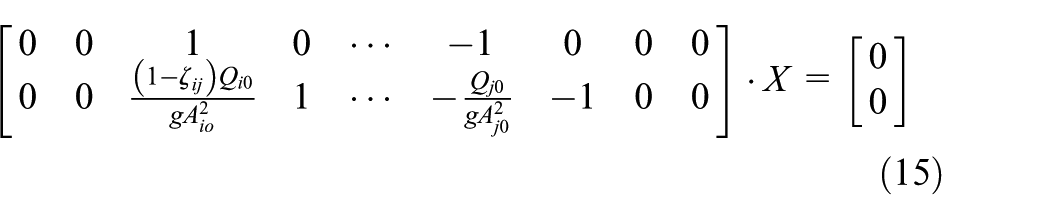
where N represents the total number of pipes and channels. The point transfer entries for the joint between pipe sections i and j lie in rows
Boundary treatments at the confluence of branch channels
Like pipe and channel junctions, the branch-channel confluence is modeled by the continuity and energy equations at the outlet, given in equation (16)
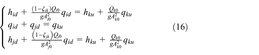
where i, j represent branch channels and k represents main tailrace.
Taking the local hydraulic loss at the end of the branch into account, the linearization of the hydraulic loss term results in
The sub-matrix blocks of the convergence of branch pipe sections can be obtained from equation (16), as shown in equation (17)
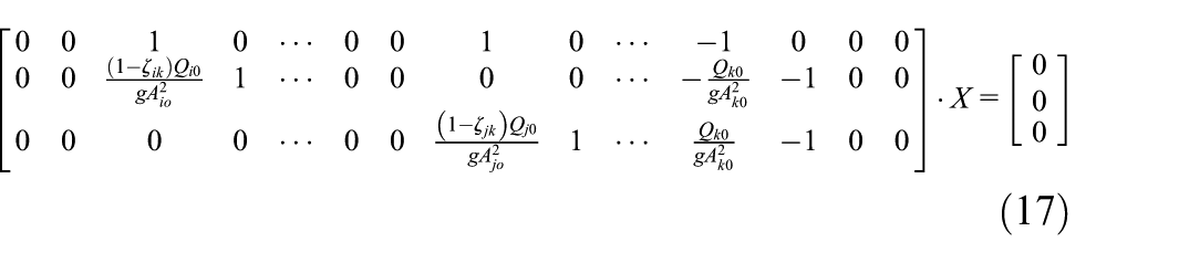
The confluence of Branch Channels point transition matrix entries occupy rows
Boundary treatment of the tailrace outlet
In the study of hydraulic transitivity, the ideal downstream reservoir method that assumes the tail water outlet boundary as having no head fluctuation (
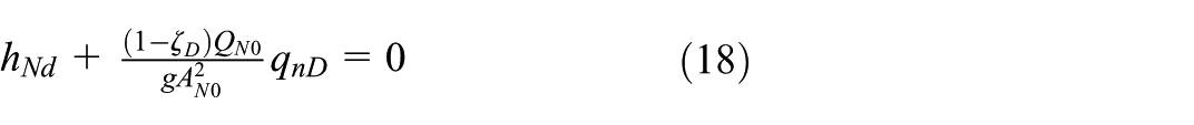
In the formula, N counts all pipes and channels within the tailrace system.
The tailrace outlet boundary submatrix block can be transformed by equation (18), as shown in equation (19)
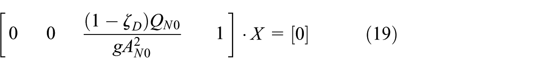
The point-transition-matrix entries for the tailrace outlet occupy row
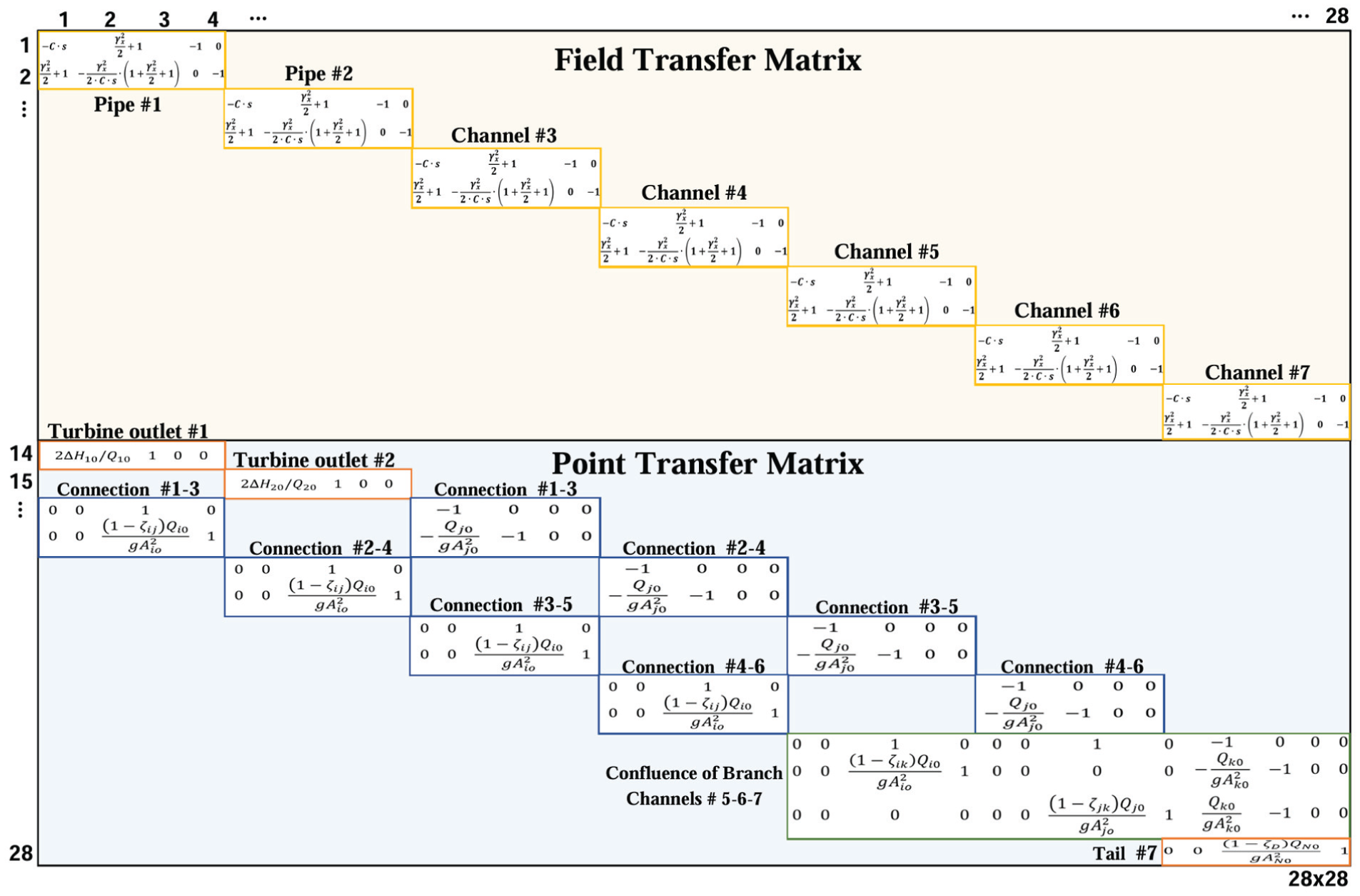
The networked transfer matrix.
Steady-state flow calculation of the system
To establish the networked transfer matrix of the system, it is also necessary to calculate the system state under the reference steady state. The mathematical expression of the stable flow in the open channel is shown in equation (20) (Nicolet et al., 2007)
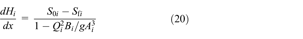
With the flow steady, the open-channel velocity stays uniform. Hence, if the depth at one end of the channel is known, equation (20) gives the depth all along it. In this study, the numerical solution is obtained using the classic fourth-order Runge–Kutta approach (Streeter, 1967; Zheng et al., 2021).
The stable flow equation of the pressurized pipeline is shown in equation (21)
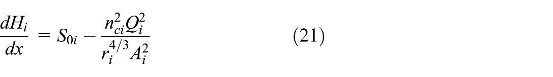
Because
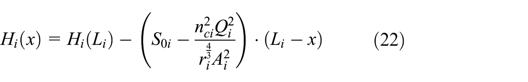
In the formula,
System stability analysis
This study concentrates on analyzing how the system behaves when operating close to its reference equilibrium. This system has 28 state variables, and the network system matrix
Owing to the mixture of transcendental and algebraic functions of the complex frequency s embedded in the network matrix
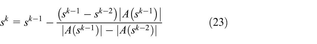
In this study, the threshold condition to end this iteration is:
The stability of the tailrace system was analyzed by using the proposed frequency-domain discrete equivalent circuit model. Simulation calculations were carried out for two operating scenarios: the load variation process of a single unit and the synchronous load variation process of two units. The calculated critical point of system stability was compared with the measured data of the power station to verify the validity of the simulation. The stability analysis process is as follows:
Step 1. The system model matrix is solved using the Newton–Raphson iterative method to obtain the corresponding system solutions at different power levels.
Step 2. Convert the actual measured ultra-low frequency oscillation frequency of the power station into radian frequency and find the solution corresponding to the given radian in the imaginary part of all system solutions.
Step 3. Judge system stability based on the real part of the solution: If the real part is < 0, the system is stable. Otherwise, the system is unstable.
Case I: Single-unit load reduction process
Throughout the Case, Unit 1 remained at 190 MW while Unit 2 was steadily unloaded from 180 to 100 MW. During the load reduction process, the power of Unit 2 was successively stabilized at 170, 150, 130, 110, and 100 MW. Each stage lasted approximately 200 seconds, with the entire process lasting roughly 900 seconds.
Due to the presence of environmental noise during the actual test, which significantly affected the collected data, the measured data in this study underwent noise reduction processing. The denoising approach leverages the widely used fast Fourier transform (FFT) technique. The sampling frequency is 10 Hz. The power threshold to remove the high-frequency noises is chosen as 0.001 (Luchtenburg, 2020). The raw data from the entire measurement process and the corresponding noise-reduced data are presented in Figure 3.
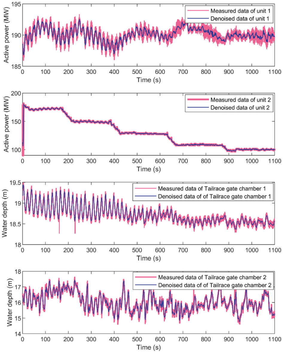
Comparison of measured data and noise reduction data during the load variation process of a single machine.
Seen from Figure 3, before 670 seconds (the stage when the active power of Unit 2 was > 110 MW), the water depth presented quasi-sinusoidal periodic fluctuations with a large amplitude (about 0.3 m). During the load decline process, periodic water depth fluctuations lasted until Unit 2 reached a steady state of 110 MW. With Unit 2’s load being reduced, the oscillation fades in amplitude and its shape departs from the original pattern. Due to the decrease in the total output of the system, the flow rate of the tail water in the main tunnel has decreased, and the water depth of both sluice chambers has presented a downward trend.
As shown in Figure 3, the downward trend of the water level in the measured data of Tailrace gate chamber 2 is not obvious. We think there is an error in the sensor measurement at tailrace chamber 2. The actual situation should be similar to tailrace chamber 1 and has a downward trend. Due to the above reason, all stability in this study rely on measurements acquired at Tailrace Chamber 1.
To clarify the long-term depth-oscillation trends, we applied a Savitzky–Golay smoothing filter that locally fits least-squares polynomials to suppress high-frequency noise (Krishnan and Seelamantula, 2012). This filter was used to separate the DC component from the denoised time series data of water depth, while preserving the AC component. Filtering was performed with a third-order polynomial and a 1001-point window. The obtained AC component was subjected to spectral analysis, resulting in Figure 4.
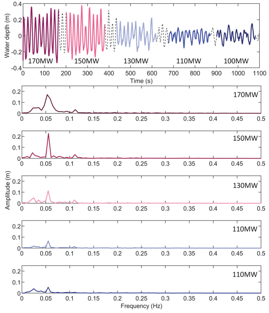
Water depth AC component and FFT transform data.
Seen from Figure 4, with Unit 1 held at constant output while Unit 2 is dispatched at 130 MW, 150 MW, and 170 MW, the amplitudes of the component with a frequency of f = 0.058 Hz are relatively prominent, being 0.11, 0.20, and 0.16 m, respectively, while the other frequency components amplitude are significantly lower. Analysis shows that within the 130–170 MW window, oscillation mode is approximately periodic oscillation. When the unit operates under the conditions of 110 and 100 MW, the frequency of f = 0.058 Hz amplitude drops to approximately 0.05 m, which is significantly weakened compared with the operation under the conditions of 130–170 MW. At this time, the amplitude difference between this frequency component and other frequency components is no longer significant, and the measured data curve does not show a sharp fluctuation amplitude and obvious periodic oscillation characteristics. It is determined that the system is in the stable operating range under this working condition. There is an error between the 0.058 Hz obtained from the calculation simulation and the measured ultra-low frequency oscillation frequency of 0.0625 Hz. The analysis suggests that it may result from the unmodeled dynamic characteristics of the system, the parameter uncertainty of the hydraulic components, and the measurement errors in the field experiments.
System stability analysis of Case I
The Unit 1 flow rate is set to Qt1 = 320 m3/s, P1 = 190 MW. The Unit 2 active power decays from 200 to 80 MW, and its flow rate changes accordingly. Based on the measured data of the power station, the ultra-low frequency oscillation frequency is 0.0625 Hz, and the converted angular is approximately 0.3926 rad/s. When conducting the system stability analysis using the networked transfer matrix, all solutions
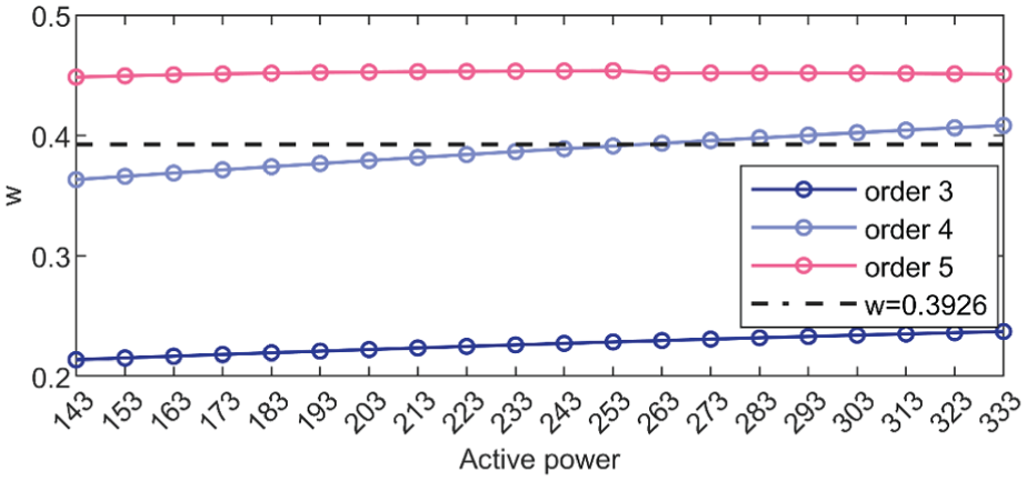
The values of the third to fifth orders in the stability analysis solution.
Among all eigen-solutions, the fourth mode’s natural frequency lies nearest to the observed ultra-low-frequency oscillation. Therefore, the fourth-order solution is retained as the benchmark for stability analysis. The flow rate Qt2 and σ relation curve of Unit 2 was plotted using the fourth-order real part calculation results under different working conditions, as shown in Figure 6. When σ < 0, the system is stable; otherwise, it is unstable.
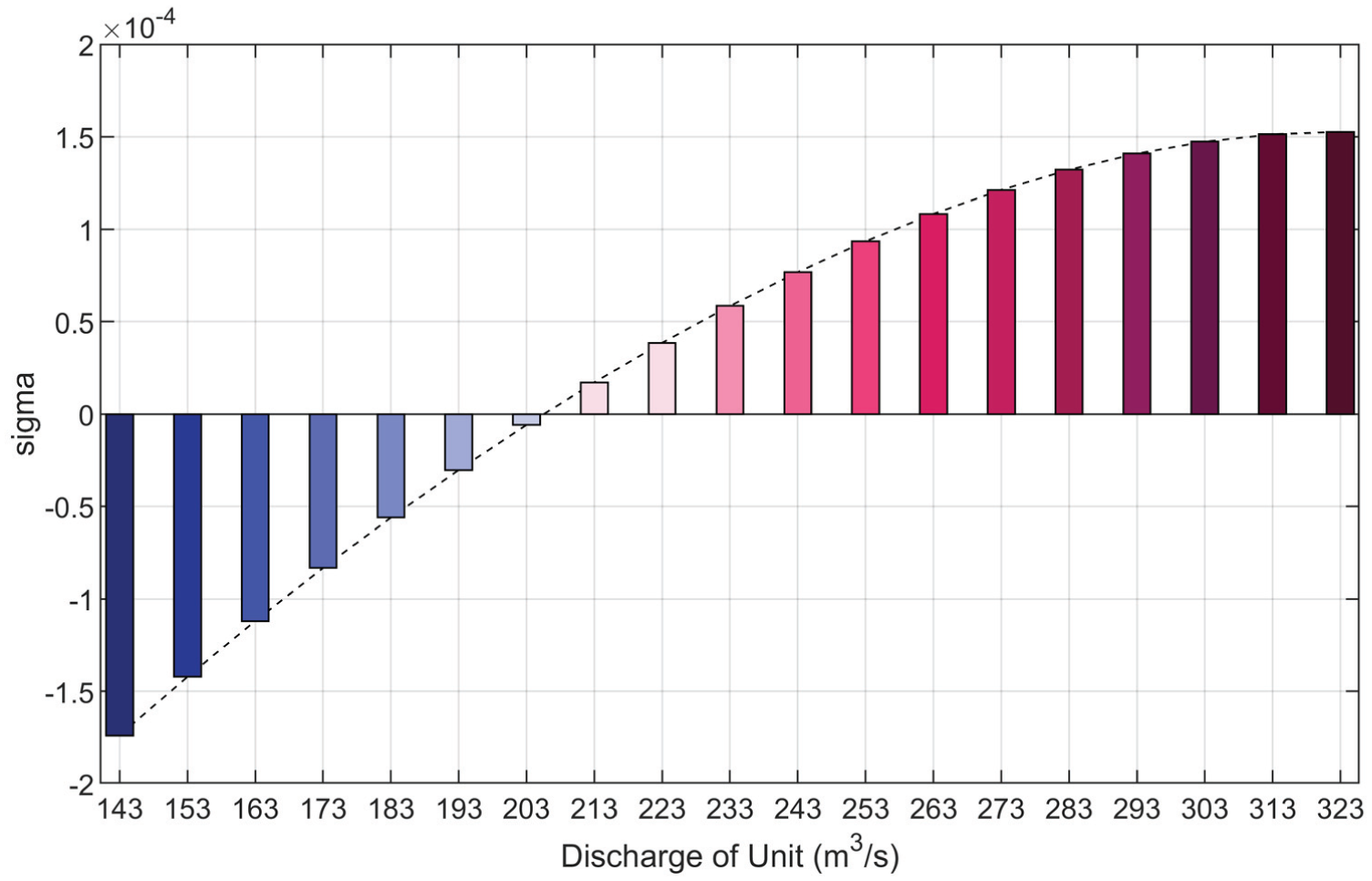
Relation curve of Qt2 and σ4 for Case I.
Figure 6 can clearly determine the turning point of system stability, at which the corresponding critical flow rate is Qt2 = 205 m3/s (126.6 MW). Comparison with Figure 4 shows that at 110 MW from Unit 2, the system lies on the stable side of the boundary; at 130 MW, it loses stability. The critical working conditions calculated by the networked transfer matrix model are consistent with the actual power station data. Thus, it can be inferred that when the actual water flow exceeds the theoretically predicted station-instability boundary, the system becomes unstable; when it is lower than this boundary, it remains stable. This result confirms the consistency between the experimental data and the theoretical solution in this case.
Case II: Double-unit load decline process
The measurement data of two units load reduction process are shown in Figure 7. The active power of two units is set to 180 MW at the beginning and then it synchronously decreases from 180 to 120 MW within approximately 1000 seconds. During the entire process, the active power of the two units stabilized at 150, 140, 130, and 120 MW successively. Similar to Case I, the original data was denoised, and the original and denoised data of double-unit load decline process is shown in Figure 7.
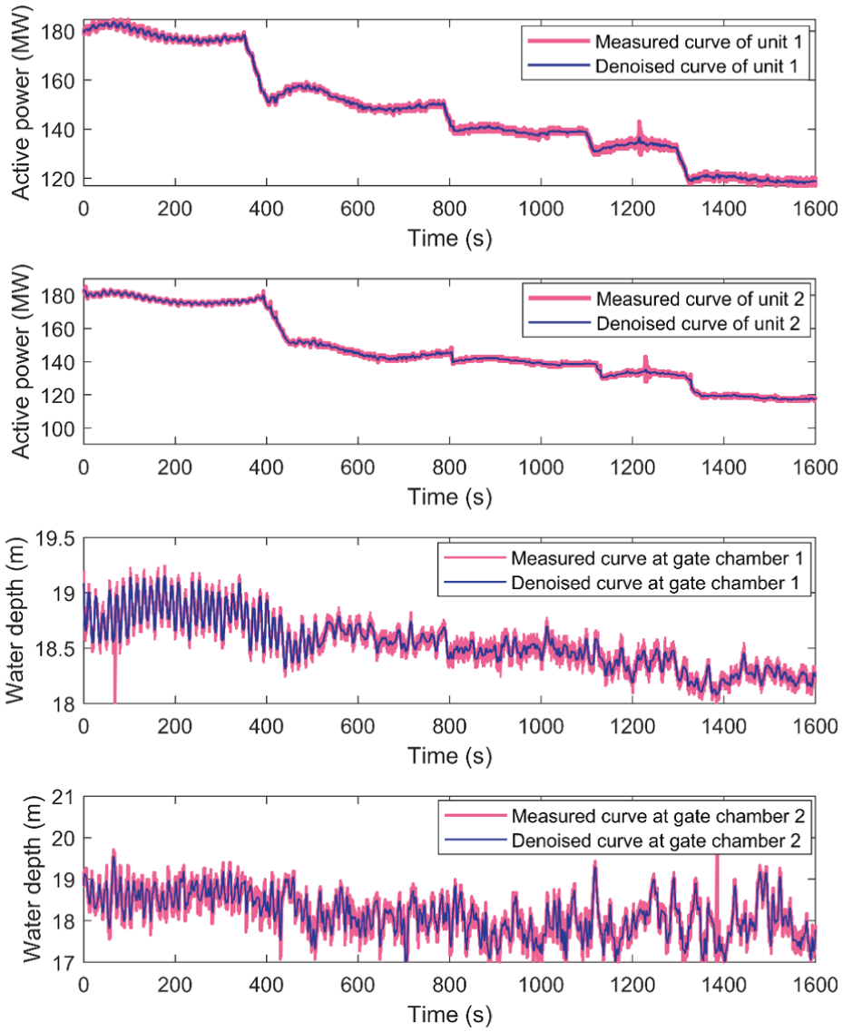
Original and denoised data of double-unit load decline process.
During the entire load decline process, periodic water depth oscillations continue until active power at 150 MW, beyond this point the amplitude drops sharply and the period becomes indiscernible. At the same time, due to the reduction in the power output of the two units, the main tailrace tunnel flow rate decreases accordingly, and the water levels in both gate chambers fall in step.
In order to better understand the variation law of water depth oscillation, similar to Case I, the DC component curve was removed while the AC component curve was retained and spectral analysis was conducted on it. The result is shown in Figure 8.
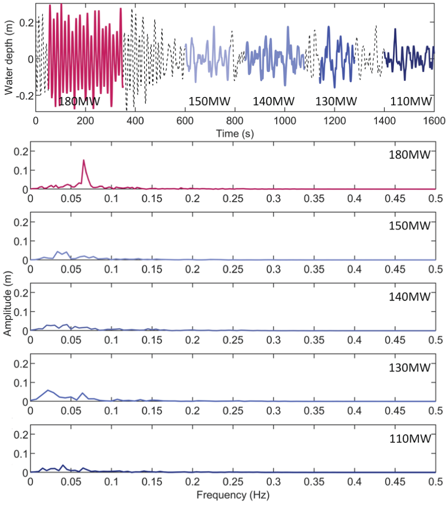
Water depth AC component and FFT transform data.
Figure 8 shows that under during the condition of 150–180 MW, the 0.0657 Hz component dominates with an amplitude of approximately 0.15 m and other frequencies being markedly attenuated. This points to an almost periodic depth-oscillation mode under this load. At 110–150 MW, the 0.0657 Hz peak shrinks markedly and the spectrum flattens, showing no dominant component. Therefore, the stability boundary is taken to lie in the 150–180 MW range. There is an error between the 0.0657 Hz obtained from the calculation simulation and the measured of 0.0625 Hz. This discrepancy is attributed to unmodeled dynamics, uncertain hydraulic parameters, and field-measurement error.
System stability analysis of Case II
The flow rate is set to Qt1 = Qt2 = 323 m3, and then simultaneously decrease from 323 to 193 m3, which is equivalent to the active power of the two units simultaneously decreasing from 199 to 119 MW. Similar to Case I, the measured data of the power station shows that the ultra-low-frequency oscillation frequency is 0.0625 Hz, and the converted arc is approximately 0.3926 rad/s. When conducting the system stability analysis using the networked transfer matrix, all solutions
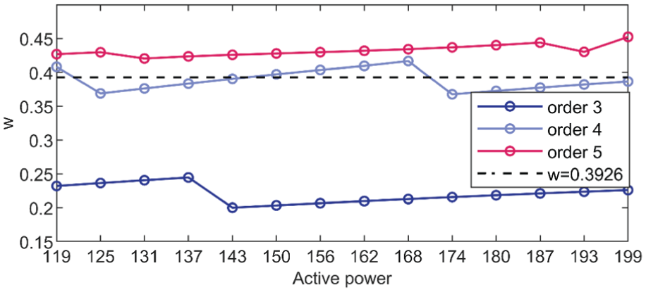
The values of the third to fifth orders in the stability analysis solution.
Among all eigen-solutions, the fourth mode’s natural frequency lies nearest to the observed ultra-low-frequency oscillation. Therefore, the fourth-order solution is retained as the benchmark for stability analysis.
The flow rate Qt2 and σ relationship curve of Unit 2 under various operating conditions was plotted using the fourth-order real part results and is shown in Figure 10. When σ < 0, the system is stable; otherwise, it is unstable. Figure 10 can clearly determine the turning point of system stability, at which the corresponding critical flow rate is Qt2 = 243 m3/s (149.9 MW). Comparing with Figure 8, this shows that at 150 MW, the system lies on the stable side of the boundary, but it becomes unstable when it comes to 180 MW. Similar to the conclusion of Case I, it can be inferred that when the actual water flow exceeds the theoretically predicted station-instability boundary, the system becomes unstable; when it is lower than this boundary, it remains stable. This result confirms the consistency between the experimental data and the theoretical solution in this case.
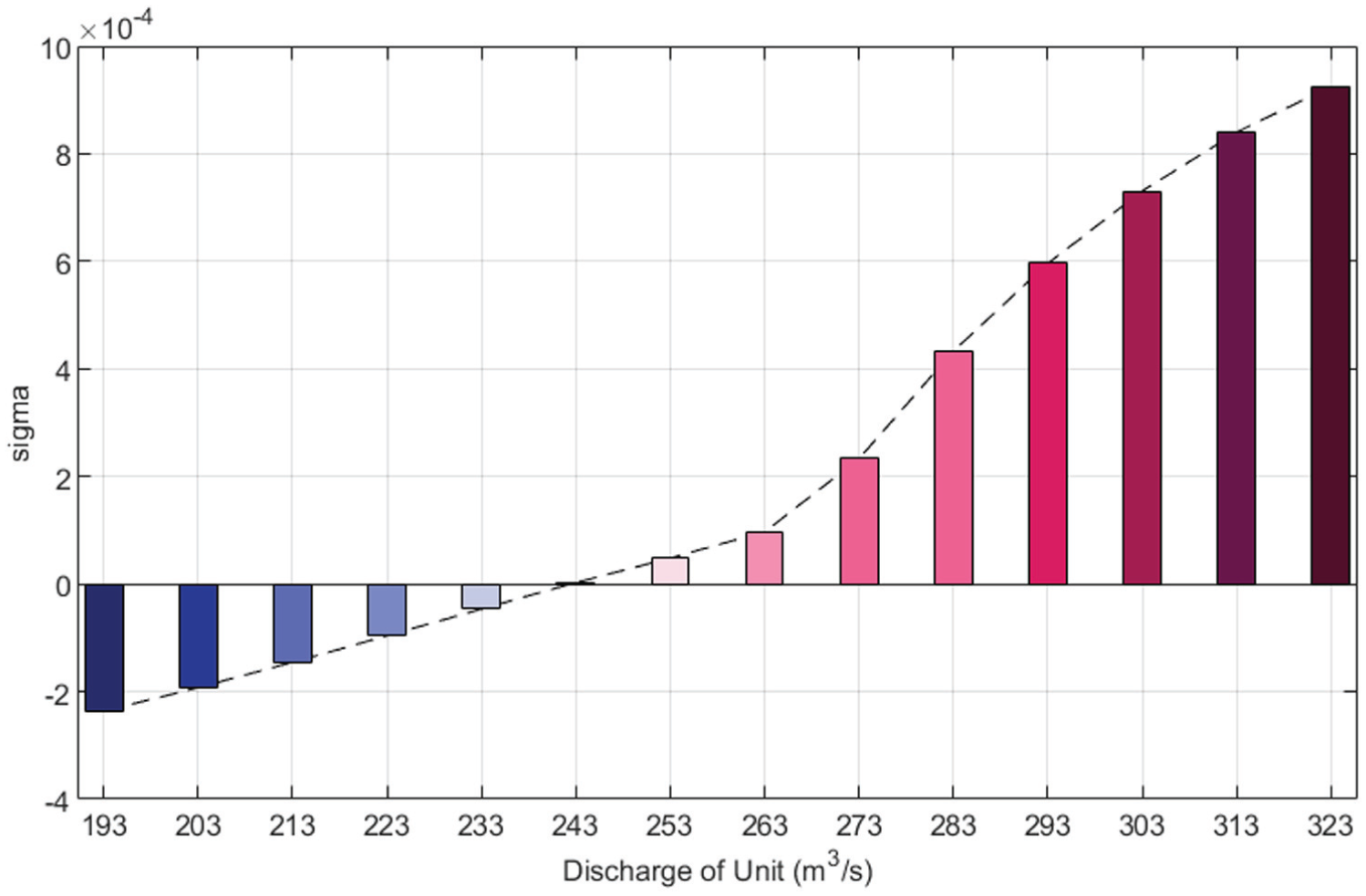
Relation curve of Qt2 and σ4 for Case II.
As shown in Figures 6 and 10, the critical stability flow rate is 205 m3/s for a single unit, corresponding to 126.6 MW. The critical stability flow rate is 243 m3/s for double units, corresponding to 149.9 MW per unit. We believe that the stability difference between single-unit and dual-unit systems is affected not only by operating conditions but also by hydraulic structures, water head, power level, and so on.
The two case studies adopted in this study are actually complex and long processes composed of multiple working conditions. Each case includes the entire process of the unit power reductions from high load condition to low load condition, and the data recording time of the entire working condition lasts for a relatively long time, approximately 1100 seconds. During this process, the variation range from high load to low load of the power station is already included. We believe that the two operating conditions introduced in the article cover the common operation range of the power station, which can verify the reliability of the conclusions.
Conclusion
Focused on the flow-induced ultra-low-frequency oscillation of the hydropower unit, this paper conducts research on the modeling and stability analysis of the hydraulic dynamic characteristics of the power station tailrace system combining open and full flows. First, a frequency-domain modeling method based on circuit equivalence is proposed, which shows strong adaptability for complex pipeline systems. Second, the exact oscillation order of the observed ultra-low-frequency oscillation is first identified determined from using the measured data spectra, and the corresponding dominant eigen mode is then obtained. By tracking the eigenvalue of this specific mode, the precise stability boundary can be obtained calculated without scanning all the eigenvalues of all oscillation modes of the system. Two on-site experiments were conducted to reveal the change law of the ultra-low frequency oscillation in the hydropower station located in southwest China. For the single unit, the results indicate that the actual critical power during single-unit load decline is between 110 and 130 MW, while the critical power calculated by the proposed model is 126.6 MW. For the double-unit load decline condition, the measured critical power is approximately 150 MW, and the simulated value is 149.9 MW. The simulation results demonstrate that the predicted system stability turning points under different operating conditions are in good agreement with the field-measured data, which verifies the accuracy of the proposed frequency-domain model. The proposed stability analysis scheme can thus help judge the operational safety of complicated hydraulic systems.
Nevertheless, the proposed method relies on detailed structure and parameters of the hydraulic design in the hydropower plant and is limited to steady-state stability analysis. The dynamic stability analysis of transient processes will be further explored in future research.
Footnotes
Appendix 1
Appendix 2
2. The system basic parameters.
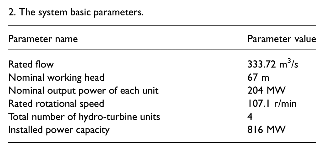
| Parameter name | Parameter value |
|---|---|
| Rated flow | 333.72 m3/s |
| Nominal working head | 67 m |
| Nominal output power of each unit | 204 MW |
| Rated rotational speed | 107.1 r/min |
| Total number of hydro-turbine units | 4 |
| Installed power capacity | 816 MW |
Author contributions
Funding
The authors disclosed receipt of the following financial support for the research, authorship, and/or publication of this article: The authors are deeply grateful that this work was funded by the National Natural Science Foundation of China (Grant No. 52579089).
Declaration of conflicting interests
The authors declared no potential conflicts of interest with respect to the research, authorship, and/or publication of this article.
Data availability statement
Data will be made available on request.