
Abstract
To improve the prediction accuracy of the remaining useful life of bearings, this study proposes a neural network model that incorporates expert knowledge embedding and periodic identification methods. In the proposed architecture, expert knowledge features are first extracted from raw vibration data and embedded into a high-dimensional space. A trend decomposition module is then implemented for data augmentation, followed by a periodic identification module to capture characteristic periodicities. Subsequently, a sequence-to-sequence architecture is adopted for the final remaining useful life prediction. The effectiveness of the model is validated through accelerated bearing life experiments. Experimental results demonstrate that the proposed approach achieves superior performance on the publicly available PHM2012 dataset, outperforming existing state-of-the-art methods. Furthermore, it obtains even better performance on a proprietary accelerated bearing life test dataset, confirming its strong generalization capability across varying operating conditions. Ablation studies further verify the individual contributions of the integrated modules to the overall robustness of the model. These findings establish an effective framework for predicting the remaining useful life of critical rotating components in mechanical systems, highlighting its significant potential for practical predictive maintenance applications.
Keywords
Introduction
Rolling bearings are critical rotating components in transport equipment, including high-speed trains, automobiles, and ships. In the context of Industry 4.0, transport equipment must operate continuously under heavy loads and harsh conditions, making bearing reliability a paramount concern (Chen et al., 2020; Lei et al., 2007; Li et al., 2023). Traditional Prognostics and Health Management (PHM) techniques, which rely on preventive and corrective maintenance, often result in either insufficient or excessive maintenance. To reduce operational costs, PHM technology is transitioning toward intelligent solutions. The health condition of bearings directly influences economic efficiency and social safety. Consequently, effectively monitoring bearing operating conditions and accurately predicting the remaining useful life (RUL) are essential for extending equipment lifespan and preventing catastrophic losses.
Techniques for predicting the RUL of bearings are generally categorized into model-driven and data-driven approaches. Model-driven methods rely on expert knowledge, such as vibration analysis (Yu et al., 2024), operational mechanisms, and probabilistic statistics (Li et al., 2025), to construct models that offer strong interpretability (Chen et al., 2013). Traditional RUL prediction methods are typically based on three types of models (Wesley Hines and Usynin, 2008): failure data (Zhang et al., 2018), stress data (Wang et al., 2015), and degradation effects (Peng and Dong, 2011). However, the complexity of mechanical systems and the prevalence of unpredictable operating conditions often limit the ability of analytical models to accurately reflect real-world degradation scenarios. Consequently, data-driven methods have garnered significant attention in recent years.
Early data-driven methods frequently integrated expert knowledge with machine learning techniques. For instance, Wahyu et al. (Caesarendra et al., 2011) employed probabilistic methods and support vector machines (SVMs) to predict fault degradation, whereas Tan et al. (2023) introduced normalized balanced multi-scale entropy for identifying bearing fatigue states. Furthermore, constructing reliable health indicators and dynamically setting failure thresholds have proven crucial for tracking degradation. For example, Li et al. (2022) proposed a comprehensive RUL prediction approach based on risk assessment and degradation state coefficients. By utilizing variational mode decomposition-singular value decomposition (VMD-SVD) and Mahalanobis distance, they constructed a monotonic health indicator, which was successfully combined with support vector regression for accurate life estimation. These approaches have characterized the degradation of mechanical components by leveraging traditional expert knowledge, providing innovative solutions to overcome the limitations of conventional methods. In comparison, deep learning enables more accurate and efficient predictions of bearing RUL, reducing costs and risks while aligning with technological advancements. Deep learning models, including convolutional neural networks (CNNs) (Cao et al., 2021; Chen et al., 2022; Wang et al., 2021), recurrent neural networks (RNNs) (Ma et al., 2024; Mao et al., 2018; Yao et al., 2022), graph neural networks (GNNs) (Wei et al., 2023; Xiao et al., 2024; Yang et al., 2022), and hybrid models (Cheng et al., 2020; Lin et al., 2023; Luo and Zhang, 2022; Niazi et al., 2024; Shao et al., 2024; Wang et al., 2023; Yao et al., 2021), have exhibited exceptional performance in the fault diagnosis and life prediction of critical components in high-speed trains.
In the field of RUL prediction, bearings typically operate in a normal state for extended durations, with their degradation process being slow and potentially spanning months or even years. This slow degradation makes it challenging to collect sufficient run-to-failure data for model training (Chen et al., 2023), particularly in industrial environments (Da Costa et al., 2020; Kim et al., 2021; Li et al., 2018). As deep learning capabilities have advanced, the primary bottleneck in RUL prediction has shifted from computational limitations to issues of data scarcity and quality. Consequently, research efforts have increasingly focused on enhancing data quality. Three key approaches have emerged: first, the use of diffusion models to generate synthetic data (Zhang et al., 2021); second, the application of transfer learning to share degradation knowledge across varying operating conditions (Zhuang et al., 2022); and third, the integration of expert knowledge by embedding calculated vibration features into models, thereby enabling the extraction of detailed degradation information from raw signals. This third approach is the central focus of this study.
Due to the stable operation of bearings during their initial stages, the available degradation information is limited and prone to noise interference, making it difficult to extract meaningful features from early vibration data. By leveraging expert knowledge to compute statistical features from raw vibration signals (e.g. root mean square, kurtosis, and peak-to-peak values), the degradation process can be characterized more effectively. To capture vibration information at each sampling point, researchers have utilized methods such as the continuous wavelet transform (CWT) (Huang et al., 2021; Zuo et al., 2023) and short-time Fourier transform (STFT) (Ma and Mao, 2021), which transform one-dimensional time series into two-dimensional time-frequency maps, preserving both temporal and spectral information. These maps are subsequently employed for feature extraction using computer vision techniques (Xie et al., 2022). Two-dimensional time-frequency representations inherently contain richer information than their one-dimensional counterparts. A similar approach has been applied to time series forecasting, where Wu et al. (2023) and Dai et al. (2023) proposed the use of the fast Fourier transform (FFT) to convert one-dimensional data into two-dimensional representations by adaptively calculating the periodicity of the time series and folding it accordingly, followed by feature extraction using 2D convolutions. Studies have demonstrated that transforming one-dimensional sequences into two-dimensional images significantly improves the extraction of critical information from the original sequences.
Motivated by these insights and challenges, this study proposes a novel hybrid RUL prediction framework that synergistically integrates expert domain knowledge with advanced deep learning architectures. The primary innovations and contributions of this work are summarized as follows:
A Multi-dimensional Expert Knowledge Embedding Layer: We develop a comprehensive feature embedding mechanism that integrates 17 classical statistical indicators (from both time and frequency domains) with temporal awareness features. This explicit embedding provides the model with prior physical knowledge, significantly enhancing feature discriminability during the early stages of degradation.
A Coarse-to-Fine-Grained Data Refinement Module: By implementing seasonal-trend decomposition (STL), we decouple the complex bearing vibration signals into distinct trend and periodic components. This “coarse-to-fine” approach enables the model to simultaneously track stable long-term degradation and capture transient variations.
Adaptive 1D-to-2D Periodic Feature Extraction: We introduce an improved TimesNet-based architecture that adaptively identifies implicit periods via the FFT. By transforming 1D sequences into 2D temporal-periodic maps, the model effectively captures intra-period and inter-period degradation patterns using multi-scale 2D kernels.
High-Performance Seq2Seq Prediction: A sequence-to-sequence (Seq2Seq) architecture with a Bi-LSTM encoder is employed to map high-dimensional features to RUL values. The effectiveness of the proposed framework is rigorously validated on both the publicly available PHM2012 dataset and a proprietary laboratory dataset, demonstrating superior accuracy and generalization over state-of-the-art methods.
Models and methods
To improve prediction accuracy and reliability, this study introduces a neural network model that integrates expert knowledge embedding with periodic identification techniques. Specifically, the model incorporates expert knowledge embedding for raw vibration data and periodic identification for feature sequences. The entire workflow, spanning from initial data collection to final RUL prediction, is depicted in Figure 1.
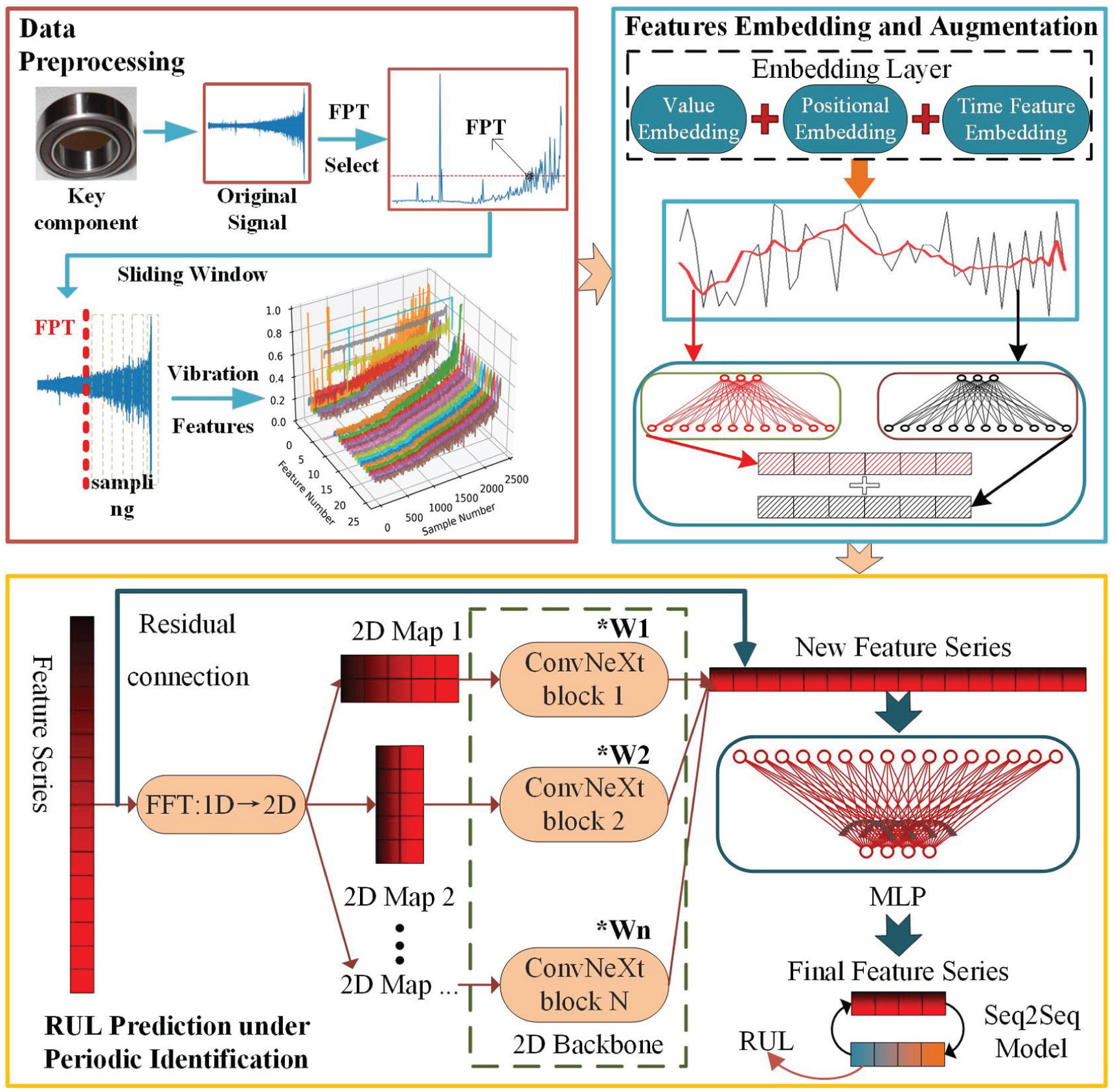
Proposed model structure.
The methodology comprises the following steps: First, data are collected from operational bearings, and the first predicting time (FPT) point is identified from the raw data using the approach outlined in Li et al. (2015). The vibration signals acquired after the FPT are then processed using a sliding window technique with a step size of one sampling file. This ensures the temporal continuity of the time windows and addresses potential data insufficiency during model training. Subsequently, drawing on prior research regarding bearing RUL prediction (Niazi et al., 2024), four categories of features—statistical, impulse, trigonometric, and frequency-domain—are extracted to provide an initial characterization of the bearing degradation process.
These extracted features are then fed into an embedding layer via a multi-feature fusion embedding method, which generates embedding values at three distinct feature scales, followed by channel mixing. This embedding mechanism is elaborated upon in the “Data collection and preprocessing” section. Next, the feature sequences are decomposed using a moving average approach. A multi-layer perceptron (MLP) is then utilized to model the coarse- and fine-grained features separately. Furthermore, the MLP is employed to expand the feature dimensions, thereby facilitating effective data augmentation.
Finally, to capture the implicit periodicity of the feature sequences, an enhanced TimesNet framework is applied for periodic feature extraction. This framework first identifies the periods of the feature sequences using the FFT, folding the one-dimensional signals into two-dimensional representations that encapsulate multiple periods. Advanced vision backbones are then used to extract multi-period features. The resulting refined features are fed into a Seq2Seq architecture for the final RUL prediction, and the model’s prediction accuracy is rigorously evaluated using established performance metrics.
Data collection and preprocessing
The data collection and preprocessing steps involve processing the original vibration signals to incorporate preliminary degradation information and transforming them into a format suitable for model input. Two primary datasets are utilized in this study: the rolling bearing dataset from the French FEMTO-ST institute (PHM2012 dataset) (Patrick Nectoux et al., 2012), which is detailed in the “Experimental setup and data description” section, and a proprietary dataset from our laboratory’s accelerated life test bench (NUAA dataset). In these experiments, a constant radial load is applied to the bearings during operation to accelerate failure, and the test is terminated when the vibration amplitude surpasses a predefined threshold.
This experimental procedure naturally encompasses both the normal operation and degradation phases of the bearings. However, the RUL prediction process specifically targets the degradation phase, meaning that vibration signals from the normal operation stage must be excluded. To ensure the model is not trained on non-degradation data, an adaptive method based on the 3σ interval (Li et al., 2015) is utilized to determine the FPT.
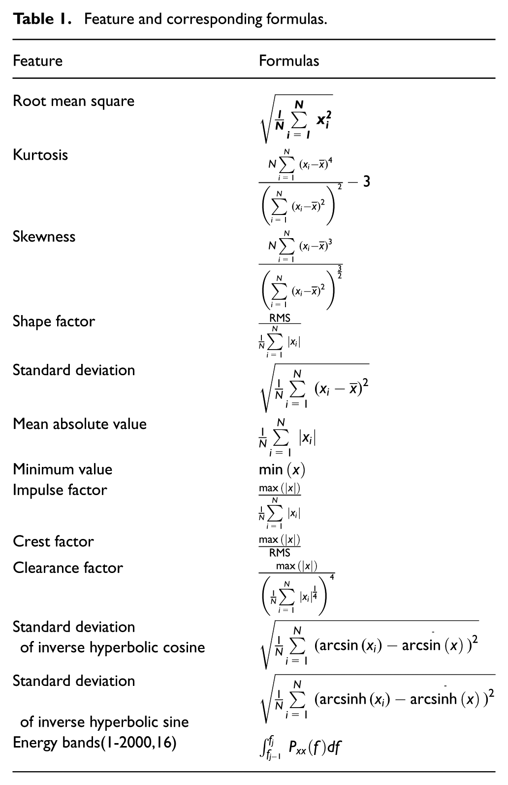
In bearing RUL prediction, the multidimensional features extracted from the raw vibration signals encompass 1D statistical, impulse, and trigonometric features, which effectively capture the dynamic and nonlinear characteristics of the signals. In addition, 1D frequency-domain features are extracted to analyze the energy distribution within specific frequency bands. These features collectively provide robust inputs for machine learning models to accurately predict the bearing RUL, thereby facilitating preventive maintenance. The specific extracted features and their corresponding calculation formulas are detailed in Table 1, where
Feature and corresponding formulas.
Feature importance analysis
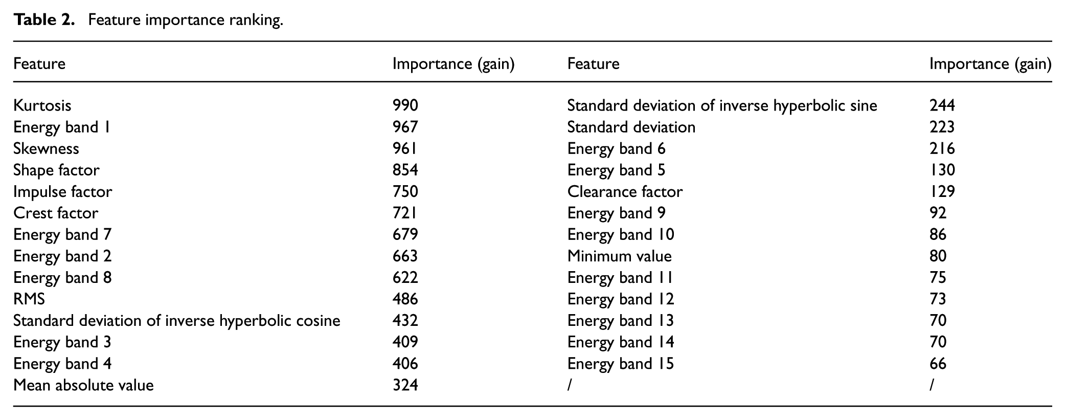
To validate the selection of the features listed in Table 1 and to understand their relative contributions to the RUL prediction task, a comprehensive feature importance analysis was conducted. We employed a LightGBM (LGBM) model—a highly efficient gradient boosting framework—trained on the PHM2012 training dataset using the full set of 27 extracted features. The importance of each feature was quantified using the “gain” metric, which reflects the total reduction in training loss contributed by that feature across all splits within the model’s decision trees. A higher gain value indicates greater predictive importance.
The results of the analysis are summarized in Table 2, which lists the relative influence of all extracted features. The full feature importance distribution is also visually represented in Figure 2.
Feature importance ranking.
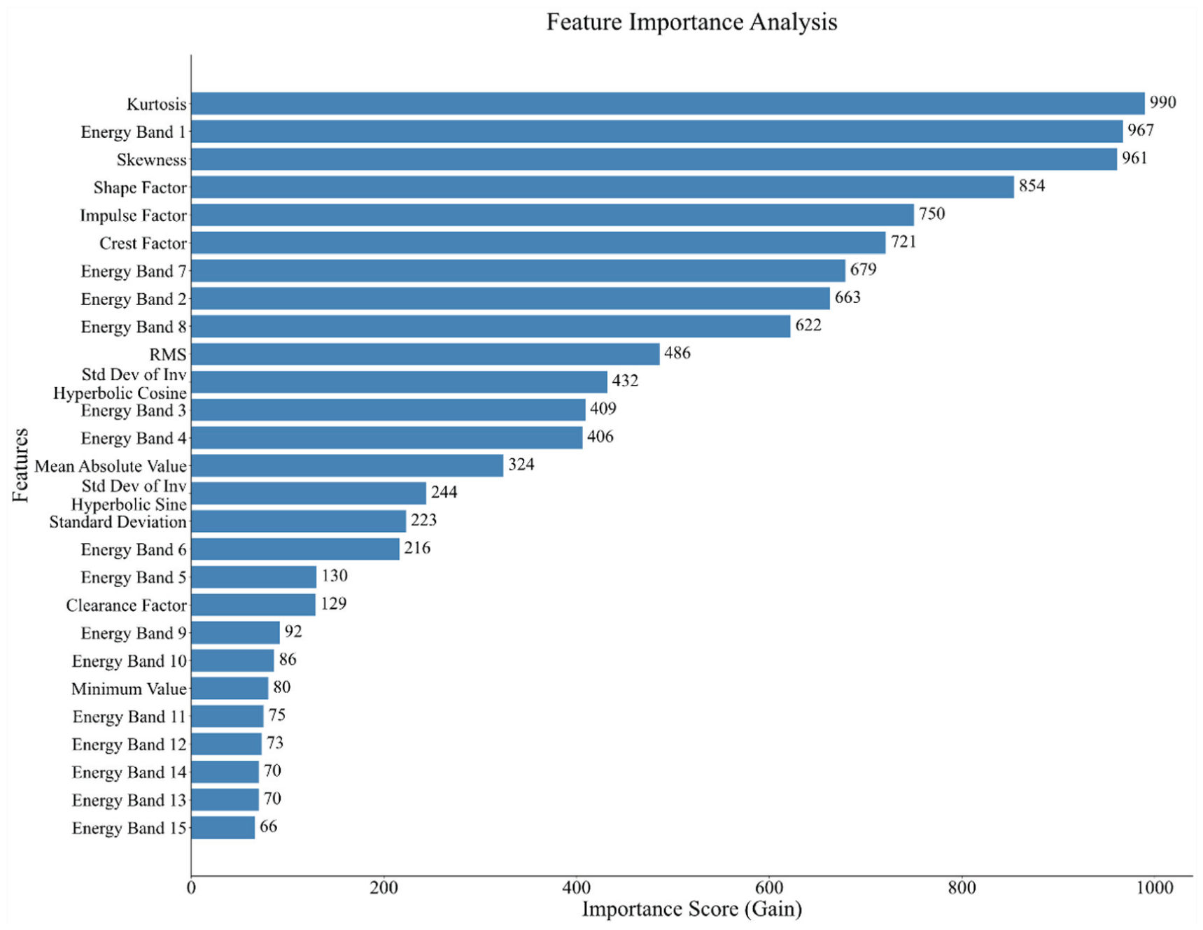
Bar plot of feature importance scores (gain) from the LightGBM model.
The analysis reveals that kurtosis and skewness are among the most critical features for RUL prediction. This finding is highly consistent with established engineering knowledge, as these higher-order statistical moments are highly sensitive to the impulsivity of a signal, which increases significantly with the occurrence of bearing spalls or cracks. Furthermore, the high importance score of Energy Band 1 confirms that shifts in the low-frequency energy spectrum serve as a key indicator of the development of faults. Other impulsivity metrics, such as the impulse factor and crest factor, also rank highly, further reinforcing this conclusion. Overall, this data-driven analysis validates that our selected feature set effectively captures the essential degradation characteristics of the bearing lifecycle.
Feature embedding and data augmentation
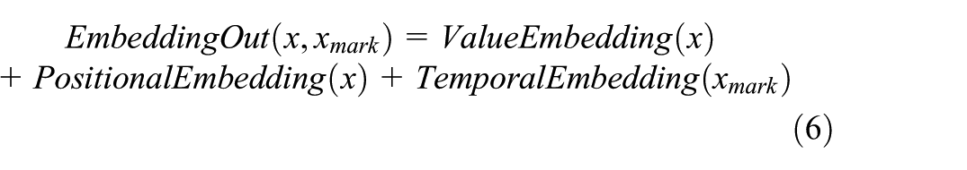
After computing the features, an embedding mechanism is utilized to map them into high-dimensional space representations. The feature embedding layer employs multi-scale fusion to integrate these features, incorporating three distinct embedding methods: value embedding, positional embedding, and temporal embedding.
Value embedding is implemented using a one-dimensional convolution (Conv1D) operation, as described by the following equation:

Here,
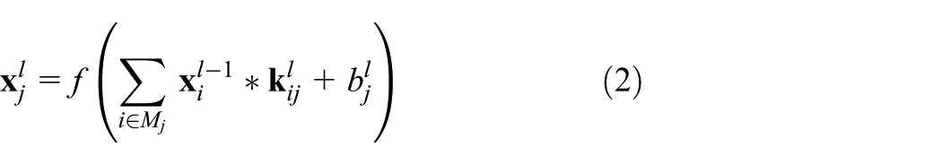
Here,
Positional embedding is designed to address the limitation of Transformer models, which inherently lack the ability to process input order. It provides multi-scale positional information using sine and cosine functions. For each position pos, the
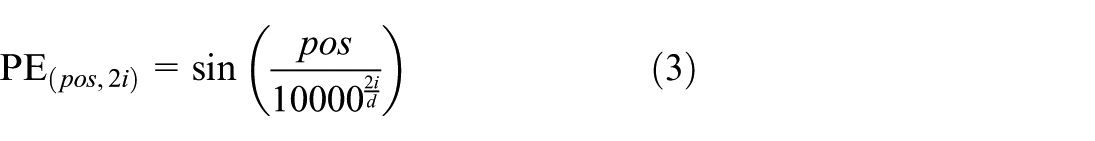
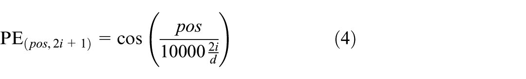
Here, pos represents the absolute position within the sequence, i is the dimension index, and d is the total number of embedding dimensions.
Temporal embedding is utilized to incorporate time-related contextual information, enabling the model to better understand the temporal characteristics of the input data. By employing a trainable embedding approach, the model adaptively learns the optimal representation of temporal features. The specific implementation is formulated as:
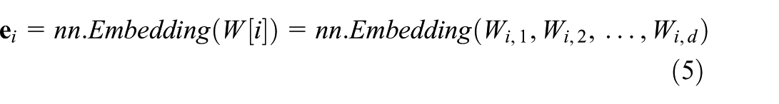
Here, is a d-dimensional vector corresponding to the -th row of the embedding matrix. The embedding vector is updated during training by optimizing the objective function, thereby capturing relationships or similarities between categories.
After passing through the three embedding layers, the model generates feature vectors at three different scales. To further enhance the feature representation, these vectors are element-wise summed. The fusion equation is defined as:
Here,
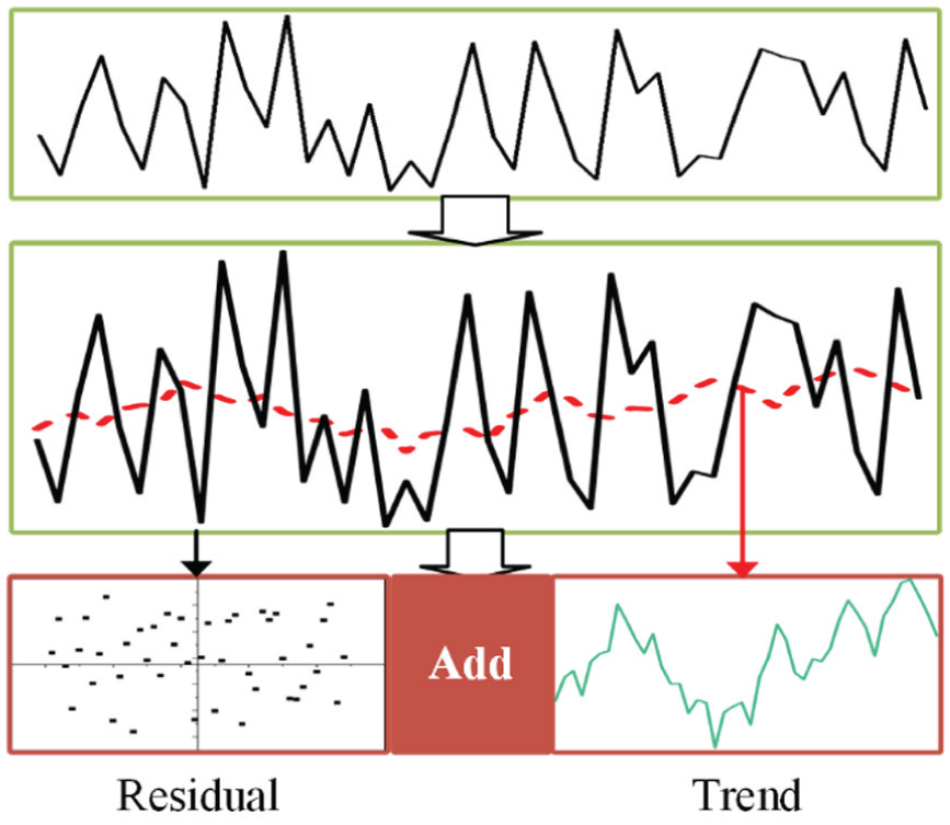
In the data augmentation stage, a novel module based on trend decomposition is introduced. Given the non-stationary characteristics of bearing vibration signals, accurately identifying the underlying degradation trend is essential for reliable RUL prediction. This module utilizes a linear decomposition model to distinguish primary degradation trends from minor perturbations that deviate from the trend. Because one-dimensional time series data typically comprise multiple components, the concepts of coarse-grained (trend, reflecting long-term degradation changes) and fine-grained (residual, representing periodic or random fluctuations) features are introduced. The decomposition process isolates these components to facilitate more precise modeling of each element, as depicted in Figure 3.
Coarse-grained modeling process.
The core concept of this method involves decomposing the original time series signal x(t) into two distinct components using a moving average filter. This filter smooths the time series data by computing the average of values within a specified window. The moving average operation is mathematically expressed as:
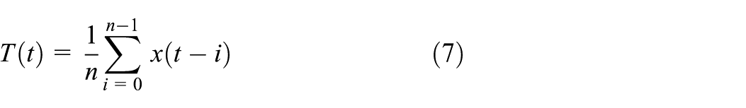
Here, n represents the window size, which determines the degree of smoothing. The trend component

Following this decomposition, an MLP is utilized to model and map the two sequences separately. The sequence length is transformed from
Remaining useful life prediction based on periodic identification
Periodicity identification is essential for detecting regular patterns that reflect underlying system behavior. This is particularly true for bearings, where periodicity corresponds to the rotational frequency and encapsulates critical health status information. The method of decoupling periodicity from a one-dimensional time series using the FFT and folding it into a two-dimensional image to capture intra- and inter-period information was initially introduced by Wu et al. and implemented in the TimesNet framework (Wu et al., 2023). However, TimesNet is tailored for long time windows (e.g. 96 or 192 time steps) in time series forecasting. This presents challenges in the PHM domain, where data scarcity makes acquiring sufficiently long time windows difficult. Building on the “Feature embedding and data augmentation” section, this study proposes a modified periodicity recognition feature extraction module based on TimesNet to better leverage the periodic information inherent in vibration data.
As outlined previously, the model utilizes a trend decomposition data augmentation module on the embedded feature sequences, extending the sequence length to align with the data structure required by TimesNet. Subsequently, by modifying the feature-weighted fusion layer in the model’s final stage, we develop a novel feature fusion layer that ultimately extracts a refined, high-level feature sequence. The feature extraction process, based on periodicity recognition, is described as follows:
First, the one-dimensional time series is transformed into the frequency domain to identify significant periodic components. The specific calculation is expressed as:
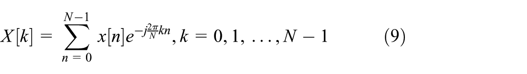
Here, N denotes the signal length, and k is a tunable hyperparameter representing the number of selected periods. The magnitude spectrum
Original Sequence: The input one-dimensional time series.
Frequency Domain Transformation: The original sequence is transformed into the frequency domain using FFT. The first value (representing total direct-current energy) is discarded, and the remaining magnitude values are averaged and sorted.
Period Selection: Based on the sorted magnitude values, the top k frequencies with the highest magnitudes are selected as the most significant periodic components.
2D Tensor: The original sequence is evenly divided into segments of equal length based on the selected periods, and these segments are then stacked into a 2D tensor.
To determine the significance of different periodic features, the weights of each period are calculated using the Softmax function after obtaining the period list from the FFT. For a selected period P, if the length T of the input sequence is not a multiple of P, zero-padding is applied to the end of the sequence to ensure exact divisibility:
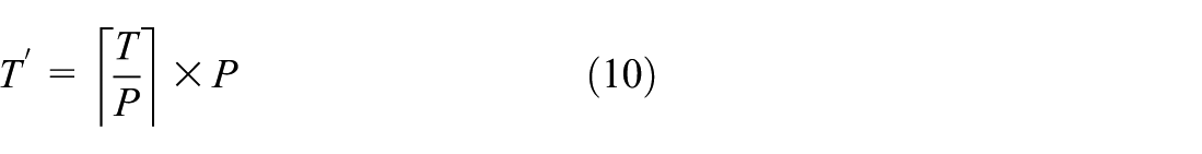
Here,
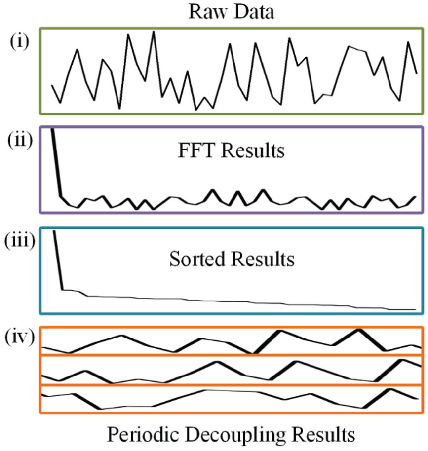
The process of FFT period detection and decoupling.
After reshaping the one-dimensional time series data into a two-dimensional format suitable for 2D convolution operations, the data are fed into the advanced ConvNeXt module (Liu et al., 2022). ConvNeXt utilizes a multi-stage design, with each stage featuring distinct feature resolutions. Its core component is depth-wise convolution, and the hidden dimension of the MLP layer is four times wider than the input dimension, effectively expanding the receptive field. This transformation enables the model to better capture multi-dimensional dependencies within periodic patterns, thereby extracting mixed intra- and inter-period features with enhanced representational capabilities.
The original TimesNet (Wu et al., 2023) was primarily designed for time series forecasting, which mandates maintaining the original temporal length for future step reconstruction. Consequently, it relies on zero-padding to align varied periodic lengths and utilizes a weighted summation to merge features. However, for bearing RUL prediction—essentially a discriminative regression task—the preservation of full temporal length through padding can introduce “semantic noise” and irrelevant zero-valued information, which may dilute the subtle degradation trends hidden in the vibration signals.
Our refinement is theoretically motivated by shifting the model’s objective from “signal reconstruction” to “high-level degradation feature extraction.” By relaxing the constraint of temporal length preservation, the model can effectively compress 1D sequences into a more compact and representative feature space, focusing strictly on the mapping between periodic patterns and the underlying health state of the bearing.
As illustrated in Figure 4, three key modifications are implemented in the feature extraction block:
Padding Elimination: The original post-convolution padding module is removed. This prevents the introduction of artificial boundaries and irrelevant information that does not reflect actual bearing wear.
Dimension Refinement via ConvNeXt: We adjust the parameters (e.g. strides and kernel settings) of the ConvNeXt module within the TimesBlock to actively shorten the feature sequence. This results in a refined, high-dimensional representation that effectively captures the “coarse-to-fine” degradation characteristics.
Weighted Concatenation: In contrast to the original weighted summation (Figure 5(a)), our model employs a weighted concatenation layer (Figure 5(b)). After multiplying features from different periods by their respective FFT-calculated weights, they are concatenated. This ensures that unique intra-period information from different frequency scales is preserved as independent features rather than being averaged out.
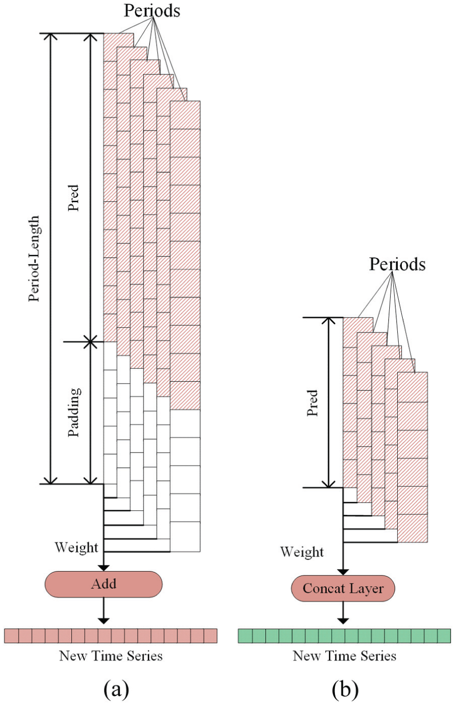
The feature extraction layer of TimesNet and the improved feature extraction layer: (a) the feature extraction layer of TimesNet and (b) improved weighted feature extraction layer.
Figure 5(a) depicts the feature extraction layer of the original TimesNet, which models and pads data from different periods, multiplies them by their respective period weights, and sums them up. Because its goal is to predict future time steps, the temporal length must remain unchanged. Conversely, Figure 5(b) illustrates the improved weighted feature extraction layer, where the parameters of the ConvNeXt module are adjusted to shorten the extracted feature length. After multiplication by the period weights, the features are fed into a concatenation layer. This ensures that essential intra-period information is preserved while reducing computational resource consumption and refining the extraction of bearing degradation features.
To validate these modifications, a comparative experiment was conducted on the PHM2012 dataset. Under identical conditions, our proposed model achieved a root mean squared error (RMSE) of 0.152 and a mean absolute error (MAE) of 0.133, significantly outperforming the original TimesNet (RMSE: 0.198, MAE: 0.175). This reduction of approximately 23.2% in RMSE confirms that our refined periodicity decoupling mechanism, combined with expert knowledge embedding, more effectively captures the critical, nonlinear degradation patterns in bearings.
Using the approach outlined in the “Feature embedding and data augmentation” section, the model adjusts the feature sequence along the time dimension while preserving degradation trend information, compressing it back to the length of the original sequence to align with the sliding window size. In the model’s final stage, a Sequence-to-Sequence (Seq2Seq) architecture is utilized to predict the bearing RUL. The Seq2Seq model is particularly effective for tasks involving sequential inputs and outputs, such as machine translation, time series forecasting, and health monitoring. By leveraging the Seq2Seq architecture, the system can capture complex temporal dependencies and generate smooth, continuous RUL curves.
The proposed RUL prediction module utilizes a bidirectional long short-term memory (Bi-LSTM) network as the encoder and a unidirectional LSTM as the decoder. During training, the encoder leverages all available data, allowing the Bi-LSTM to simultaneously capture both past and future contextual information. However, during validation and testing, the decoder naturally cannot access future data, necessitating the use of a unidirectional LSTM for the decoder architecture. To ensure the predicted RUL value is mapped to a standard range of 0–1, the decoder’s output
Network structure table.
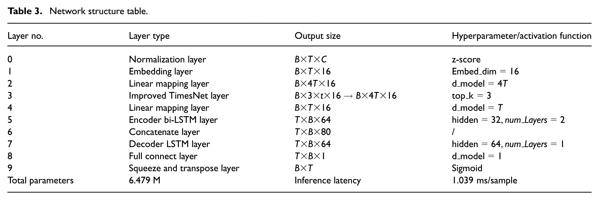
To further evaluate the feasibility of the model for real-time industrial deployment, we conducted a computational complexity analysis. The results, summarized at the bottom of Table 3, indicate that the total number of trainable parameters is 6.479 million. Performance benchmarking was conducted using a batch size of 64, yielding an average inference latency of 66.523 ± 1.907 ms per batch, which translates to approximately 1.039 ms per individual sample. With a high throughput of 962.07 samples/s, the proposed architecture easily meets the strict efficiency requirements for high-frequency real-time monitoring in embedded system environments.
Experimental results and discussion
To evaluate the effectiveness and generalizability of the proposed model, two datasets were employed: the publicly available bearing dataset from the FEMTO-ST Institute (Nectoux et al., 2012) and a proprietary rolling bearing fatigue loading dataset from our laboratory. Comprehensive comparisons were conducted against other state-of-the-art health state prediction models. The experiments were performed on a Windows 11 64-bit system equipped with an Intel Core i7-14700KF (3.40 GHz) CPU, 32 GB of RAM, and an NVIDIA GeForce GTX 1660 SUPER GPU, using Python 3.11.7 and the PyTorch 2.1.2 framework. To ensure statistical reliability, each experiment was repeated five times, and the average values of the evaluation metrics were recorded as the final results.
Experimental setup and data description
Rolling bearing dataset from FEMTO-ST Institute, France (PHM2012)
The PRONOSTIA experimental platform is designed for accelerated bearing degradation testing. It simulates real-world operating conditions by controlling bearing rotational speeds (e.g. 1800 rpm, 1650 rpm, 1500 rpm) and applying varying radial loads (e.g. 4000 N, 4200 N, 5000 N). Equipped with high-precision vibration sensors (25.6 kHz sampling rate), temperature sensors (10 Hz sampling rate), speed sensors, and force sensors, the platform monitors bearing vibration, temperature, speed, and load in real time. Each sampling period lasts for 0.1 seconds, with a 10-second sampling interval. The platform generates extensive run-to-failure data, making it ideal for developing and validating bearing condition monitoring, fault diagnosis, and RUL prediction models. This study focuses exclusively on horizontal vibration signals. The training and test sets are divided strictly according to the official PHM2012 dataset guidelines: bearings 1_1, 1_2, 2_1, 2_2, 3_1, and 3_2 are assigned to the training set, while the remaining bearings are used for testing. In addition, 20% of the training set is randomly selected to serve as the validation set.
Intelligent Diagnosis and Expert Systems Laboratory, Nanjing University of Aeronautics and Astronautics (NUAA)
The proprietary bearing fatigue loading dataset from the IDES laboratory (N. U. of Aeronautics, Astronautics, n.d.) was collected using a modified ABLT-1A bearing life accelerated testing machine, specifically designed for accelerated rolling bearing life testing. As illustrated in Figure 6, the equipment comprises a test head, test head seat, transmission system, loading system, lubrication system, and a computer monitoring system. The experiments were conducted under the following severe conditions: a rotational speed of 11,500 rpm, a radial load of 6.25 kN, a sensor sampling frequency of 30 kHz, and a sampling interval of 3 minutes. Horizontal vibration signals, collected from sensors installed on the supporting shaft, were utilized for the experiments. The dataset encompasses four experiments, each capturing data from four sets of bearings operating continuously until failure. Only data from failed bearings were included in the training set, while data from non-failed bearings were strictly excluded from both training and testing. The bearings in each experiment were labeled 1 to 4. Bearings 1 and 2 were assigned to the training set, and the remaining bearings were allocated to the test set. Furthermore, 20% of the training set was randomly selected to serve as the validation set.
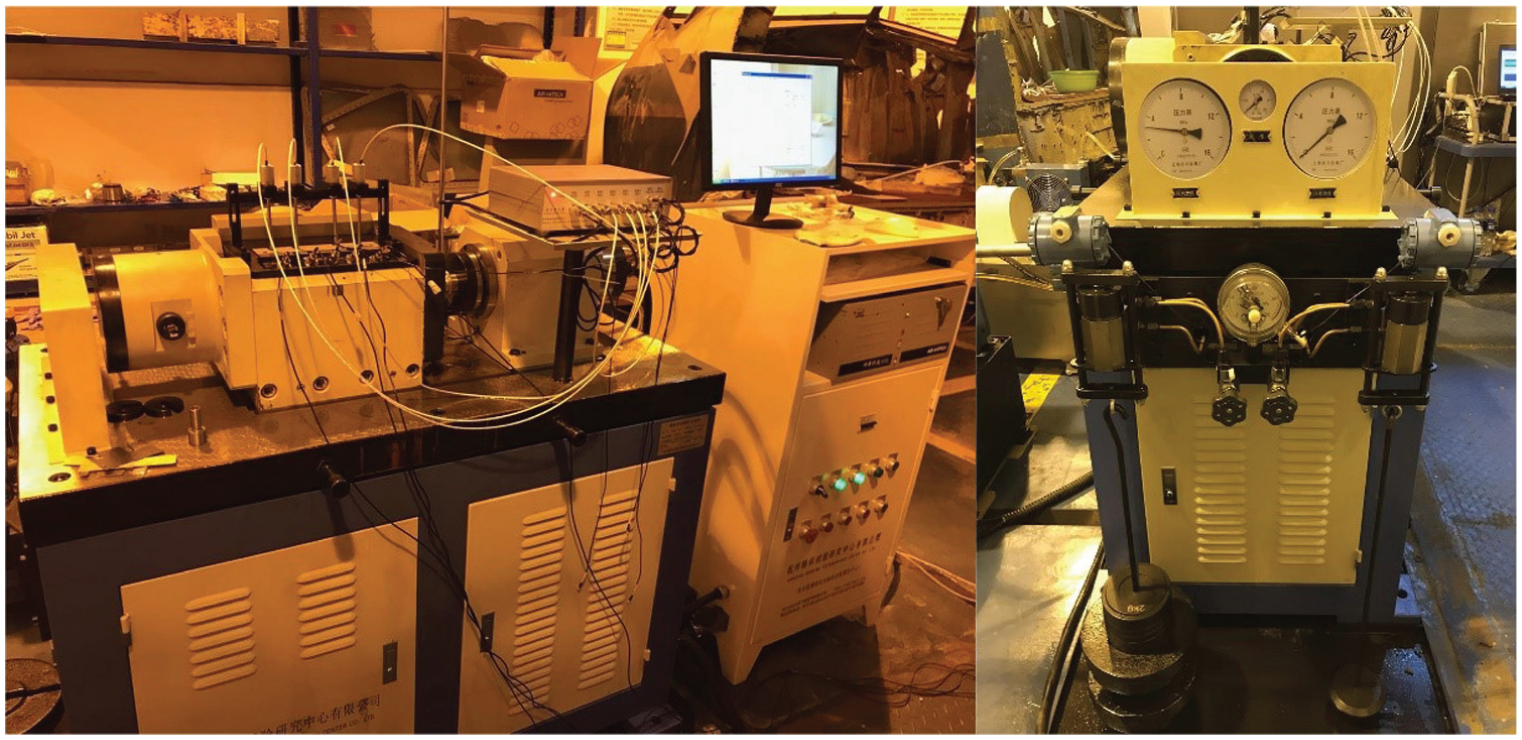
Overview of NUAA platform (N. U. of Aeronautics, Astronautics, n.d.).
Hyperparameter configuration
The selection of appropriate hyperparameters is critical for optimizing model performance and ensuring the reproducibility of our results. To this end, we employed a systematic approach to hyperparameter tuning rather than relying on arbitrary selections. Our tuning process focused on identifying the optimal set of values for key parameters that most significantly influence model training and generalization capability.
The tuning methodology involved a structured grid search over a predefined range of values for each critical hyperparameter. Specifically, we focused on the sliding window size (sequence length), learning rate, optimizer type, and batch size, as preliminary tests identified these as having the most substantial impact on validation loss. For each hyperparameter, we defined a search space, detailed in Table 4. We then systematically evaluated different parameter combinations, trained the model for each, and assessed its performance on the dedicated validation set. The configuration that yielded the lowest validation loss was selected as the optimal choice for the final model training and all subsequent comparative experiments.
Hyperparameter configuration.
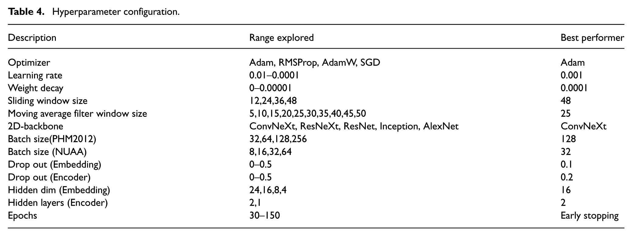
For instance, our experiments revealed that a sliding window size of 48 and a batch size of 128 yielded the best performance for the RUL prediction task on the PHM2012 dataset. The Adam optimizer, paired with an optimized learning rate of 0.001, was ultimately selected for its rapid convergence and robust performance. The complete details of the explored ranges and the best-performing values for all key hyperparameters are summarized in Table 4.
During training, the model is optimized using gradient updates via the backpropagation (BP) algorithm. The Huber Loss function is applied as the optimization objective. Huber Loss is a balanced loss function that combines the smooth optimization properties of mean squared error (MSE) for small errors with the robustness of MAE for large errors, making it highly effective for filtering outlier noise in RUL prediction. The Huber Loss function is mathematically expressed as:
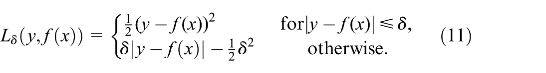
Here, y denotes the true RUL value,
Evaluation metrics
To comprehensively assess the model’s performance, three widely used evaluation metrics were employed: RMSE, MAE, and mean absolute percentage error (MAPE). The mathematical expressions for these metrics are as follows:

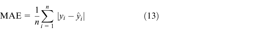
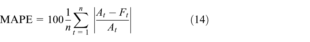
Here,
Comparative experiments
To evaluate the superiority of the proposed method over other state-of-the-art (SOTA) RUL prediction approaches, several advanced neural network models were selected for comparison using the PHM2012 dataset. These baseline models include: the ConvLSTM model, which leverages 2D features; the multi-scale time series analysis ConvLSTM (TT-ConvLSTM) model (Niazi et al., 2024); the multi-scale convolutional neural network (MLP-MSCNN) (Huang et al., 2021); and the CLSTM model (Ma and Mao, 2021), which was the first to apply 2D images for RUL prediction. Furthermore, the proposed method was compared with the Embedded Attention-based Parallel Network (EAPN) (Zhang et al., 2023) and the Memory Fusion Network (CLSTMF) (Wan et al., 2022), both of which are recognized as advanced techniques in bearing RUL prediction. Given that GCNs have shown outstanding performance in RUL prediction in recent years, we also included two state-of-the-art GCN-based methods: DCAGGCN (He et al., 2025) and DyWave-BiAGCN (Zhao et al., 2026).
As shown in Table 5, the proposed method demonstrates highly competitive performance across different operating conditions on the PHM2012 dataset. Overall, our method achieved average RMSE, MAE, and MAPE values of 0.152, 0.133, and 0.723, respectively. When compared with traditional and early 2D-based models such as MLP-MSCNN, TT-ConvLSTM, and CLSTMs, the proposed method exhibits significant improvements across most test bearings.
The detailed result for PHM2012 dataset.
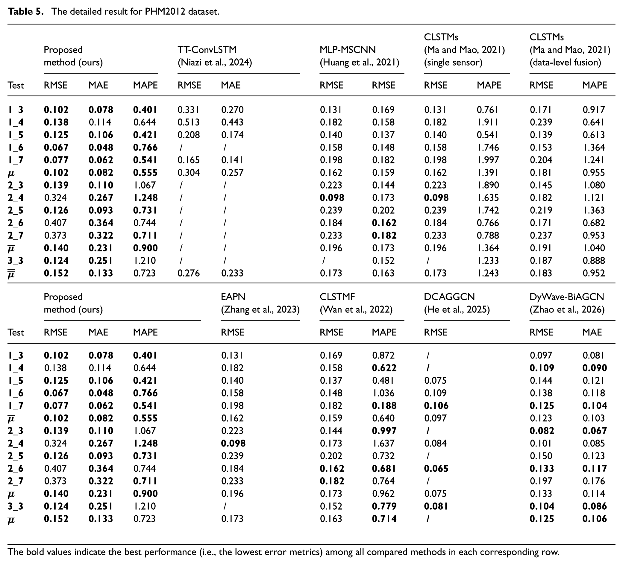
The bold values indicate the best performance (i.e., the lowest error metrics) among all compared methods in each corresponding row.
Furthermore, we evaluated the applicability of recent advanced techniques, including GCN-based models (DCAGGCN and DyWave-BiAGCN) and parallel/fusion networks (EAPN and CLSTMF). While the GCN-based methods, particularly DyWave-BiAGCN, showed outstanding predictive accuracy on certain specific test subsets (e.g. achieving lower RMSE in Condition 2), our proposed method demonstrated superior or highly comparable results under Condition 1 (e.g. test bearings 1_3, 1_6, 1_7). It is worth noting that although the proposed model did not strictly outperform the SOTA GCN models in every individual metric across all tests, it maintained a highly stable overall performance without the complex spatial graph construction typically required by GCNs. This indicates that, despite minor fluctuations in specific test cases (e.g. 2_4, 2_6), the proposed method exhibits strong robustness and generalization capabilities, ensuring reliable RUL prediction under complex and varying operating conditions.
Figure 7 presents the prediction results for test bearing 1_3 (Figure 7(a)) and test bearing 1_7 (Figure 7(b)) from the PHM2012 dataset. Since the prediction starting point is determined adaptively by a 3σ interval threshold algorithm, the timeline in the figures exclusively represents the continuous degradation phase of the bearings. To provide a detailed stage performance comparison, the absolute error values are visualized as pink shaded areas at the bottom of the figures, with lower amplitudes indicating higher prediction accuracy. In addition, a 95% prediction interval (PI) band (red shaded area) is introduced to quantify the prediction uncertainty at different stages.
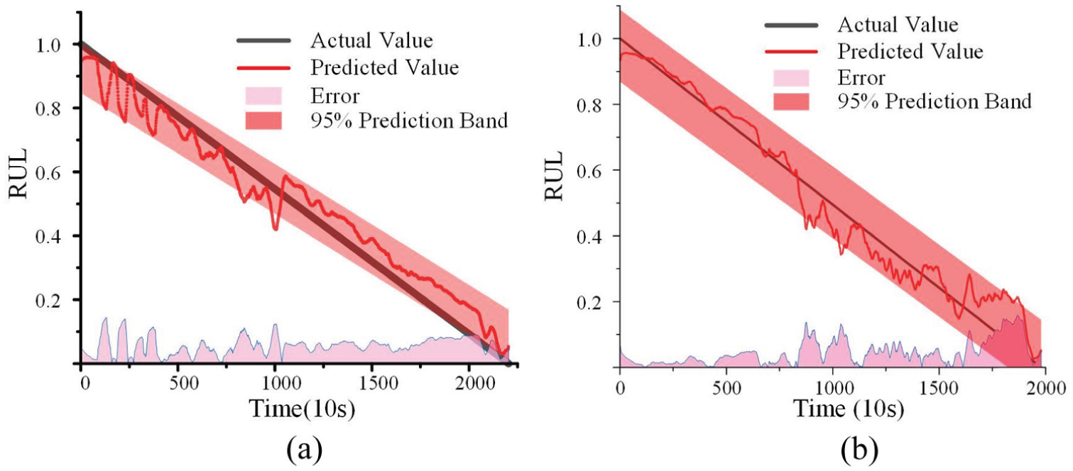
Experimental results of the proposed model: (a) experimental results of the model for PHM2012 bearing 1_3 and (b) experimental results of the model for PHM2012 bearing 1_7.
A local error analysis reveals the model’s performance across different degradation stages. For Bearing 1_3 (Figure 7(a)), the error remains relatively low and stable throughout the process. Although minor local error fluctuations occur in the early and intermediate stages (e.g. around 100–300 seconds and 800–1000 seconds) due to dynamic operational noise, the predicted values tightly track the actual RUL. More importantly, as the bearing approaches the late degradation stage (after 1500 seconds), the local error converges, indicating high reliability near the critical failure point.
For Bearing 1_7 (Figure 7(b)), the stage performance shows a slightly different pattern. In the early degradation stage (0–800 seconds), the model tracks the actual value accurately with minimal error. In the intermediate stage (800–1200 seconds), the predicted RUL exhibits a noticeable downward fluctuation, leading to a temporary peak in the local error. This indicates the model’s sensitivity to sudden, severe degradation signals captured during this period. However, in the late stage (after 1500 seconds), the model effectively self-corrects, and the prediction curve realigns with the actual RUL.
To assess whether the proposed method of decoupling signals into two-dimensional (2D) representations preserves more information than conventional approaches, a comparative experiment was conducted. The proposed signal processing technique was evaluated against traditional methods, namely the CWT and the STFT, both of which convert one-dimensional signals into 2D time-frequency representations. To ensure a fair comparison, a 2D temporal feature embedding layer was integrated into the traditional signal images to incorporate temporal information, while maintaining consistent model configurations. The experiments were validated using the PHM2012 and NUAA datasets. The comparative findings for four specific test cases—Bearings 1_3 and 1_7 from the PHM2012 dataset, and Bearings 3 and 4 from the NUAA dataset—are illustrated in Figure 8. Comprehensive quantitative results are provided in Table 6.
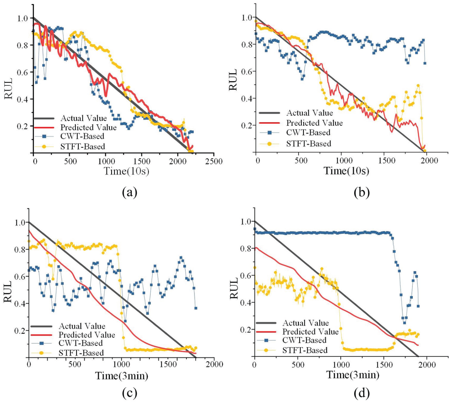
Comparison results with traditional 2D signal processing methods: CWT and STFT: (a) comparative experimental results for PHM2012 bearing 1_3, (b) comparative experimental results for PHM2012 bearing 1_7, (c) comparative experimental results for NUAA bearing 3, and (d) comparative experimental results for NUAA bearing 4.
The detailed result for PHM2012 dataset.
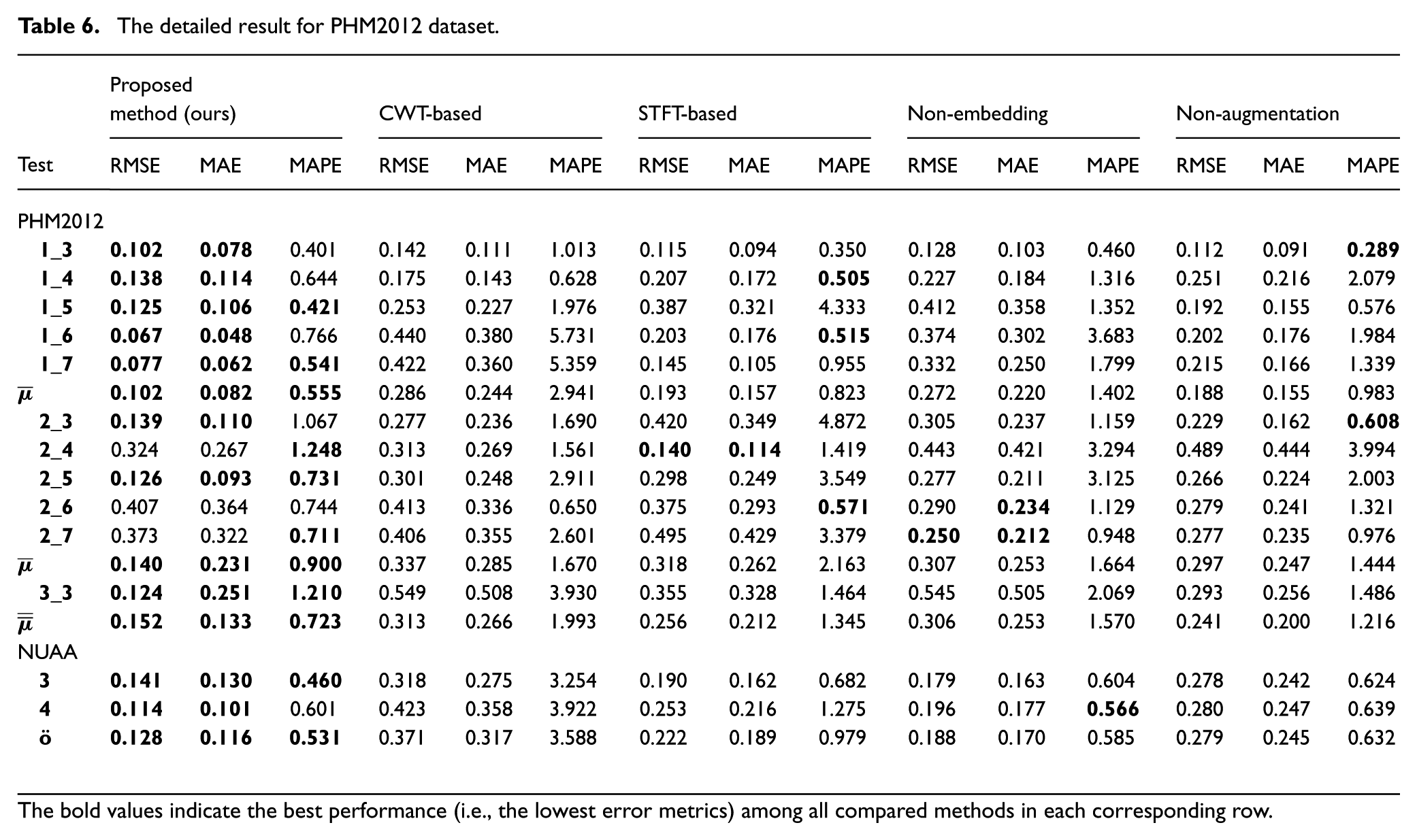
The bold values indicate the best performance (i.e., the lowest error metrics) among all compared methods in each corresponding row.
Figure 8 demonstrates that traditional two-dimensional signal processing methods are inadequate for accurately capturing subtle degradation signals within the proposed framework. The CWT-based method only captured the general degradation trend in the experiment with Bearing 1_3, where its predicted values showed significant oscillations compared to the actual values. In the other three sets of experiments, it largely failed to capture the degradation trends over time. Although the STFT-based method could broadly identify different stages of bearing degradation, it could not accurately distinguish between these stages, leading to a limited overlap between the predicted and actual values. In contrast, the proposed method exhibited significantly reduced fluctuations and generated predictions closer to the actual values, thereby outperforming the baseline methods.
Ablation study
To assess the individual contributions of the key modules proposed in this study, ablation experiments were conducted on both datasets. For each dataset, two specific ablation tests were performed: the first evaluated the role of the feature embedding layer, and the second investigated the impact of the trend decomposition data augmentation module. The experiment omitting the embedding layer aimed to validate its effectiveness in achieving robust feature representation, while the removal of the trend decomposition module sought to determine its ability to accurately capture monotonic degradation trends. For illustration, comparative plots were generated using Bearings 1_3 and 1_7 from the PHM2012 dataset, and Bearings 3 and 4 from the NUAA dataset, as depicted in Figure 9.
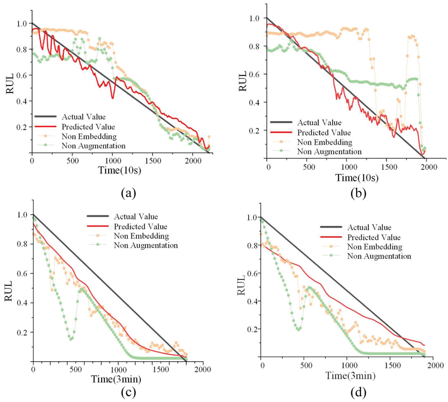
Presentation of the results of the ablation experiment: (a) ablation experiment results for bearing 1_3 from the PHM2012 dataset, (b) ablation experiment results for bearing 1_7 from the PHM2012 dataset, (c) ablation experiment results for bearing 3 from the NUAA dataset, and (d) ablation experiment results for bearing 4 from the NUAA dataset.
Figure 9 shows that, in the absence of the feature embedding module, the prediction curve (denoted by the orange squares) exhibits significant fluctuations at the beginning of the prediction, particularly in Figure 9(a). In this case, the model’s ability to track the bearing degradation process is noticeably impaired, indicating that without embedded feature processing, the model struggles to reliably capture degradation information from noisy early-stage data. When the data augmentation module is excluded, the model’s prediction curve, although smoother, still fails to consistently align with the actual RUL curve. Notably, in Figure 9(b), both ablation configurations show significant deviations in the later stages of severe degradation, highlighting the absolute necessity of the two proposed modules for accurately capturing final degradation trends. By integrating these two modules, the model achieves reduced fluctuations and closer alignment with the true values across all four test bearings. This confirms that the integration of feature embedding and data augmentation into the neural network significantly enhances prediction accuracy and stability.
As detailed in the rightmost columns of Table 6, the proposed complete method consistently achieves lower RMSE, MAE, and MAPE values across all test sets, underscoring its robustness for RUL prediction tasks. In the ablation experiments, methods lacking either the feature embedding module or the data augmentation module, despite performing moderately well on some test sets, consistently fail to match the overall accuracy of the complete proposed method. This emphasizes the critical, irreplaceable role of these modules in capturing bearing degradation trends.
On the NUAA dataset, the experimental results further validate the effectiveness of the proposed architecture. For Bearings 3 and 4 in the NUAA dataset, the proposed method achieves an average RMSE of 0.128, an average MAE of 0.116, and an average MAPE of 0.531, significantly outperforming both the CWT and STFT baseline methods, as well as the ablation models. Analysis of the comprehensive results in Table 6 confirms that the proposed method—which incorporates periodic convolutional modules guided by expert knowledge—excels in metrics such as RMSE, MAE, and MAPE. It demonstrates superior predictive capabilities, particularly in complex, multi-condition industrial scenarios.
To further elucidate the mechanisms behind these performance gains, we analyzed the specific roles and synergistic effects of the two proposed modules. The experimental results in Table 6 and Figure 9 show that the feature embedding layer is crucial for the stability of the RUL prediction, especially during the early stages of bearing operation. As seen in Figure 9(a), without the embedding layer (Non-Embedding), the prediction curve exhibits high-frequency oscillations. This occurs because raw vibration signals at the early degradation stage have a low signal-to-noise ratio (SNR). The embedding layer, which integrates 17 types of expert-defined time and frequency domain features, provides the model with a robust physical prior. This enables the network to effectively filter out non-degradation-related noise and establish a stable health indicator (HI) baseline from the outset.
Furthermore, as shown in Table 6, removing the trend decomposition module (Non-Augmentation) leads to a significant increase in RMSE and MAE (e.g. for Bearing 1_4, the RMSE increases from 0.138 to 0.251). Without decomposition, the model struggles to decouple the monotonic degradation trend from stochastic, high-frequency fluctuations. The STL-based augmentation enables the model to focus explicitly on the underlying trend component, ensuring that the predicted curve aligns closely with the ground truth even during the rapid degradation phase in the late life stage (Figure 9(b)).
Ultimately, these two modules exhibit a strong complementary relationship. The feature embedding layer enhances the discriminative capacity of multi-source signals by mapping them into a high-dimensional space, thereby significantly improving the quality of the input features. Concurrently, the trend decomposition module extracts vital temporal evolution patterns from the data. This interaction yields two key benefits: First, the improved feature quality minimizes the influence of raw signal noise, enabling a much more accurate trend decomposition. Second, the trend decomposition module generates diverse trend samples, which effectively mitigates the risk of the embedding layer overfitting to specific operating conditions. This complementary mechanism is the primary reason why the proposed method consistently achieves the lowest average errors across diverse test bearings when compared to ablation versions that utilize only a single module.
Conclusion
This paper proposes a neural network model that synergistically integrates expert knowledge embedding with a periodic identification module. Comprehensive evaluations on the PHM2012 and NUAA datasets yield the following conclusions:
The proposed model demonstrates superior RUL prediction accuracy compared to state-of-the-art approaches, achieving an average RMSE of 0.152 (PHM2012) and 0.128 (NUAA), an MAE of 0.133 (PHM2012) and 0.116 (NUAA), and a MAPE of 0.723 (PHM2012) and 0.531 (NUAA). These results confirm its robust generalization capability across diverse operational conditions.
The periodic identification module significantly enhances prediction reliability. When benchmarked against traditional signal processing methods under controlled hyperparameters and model structures, this module improves the RMSE, MAE, and MAPE by 12.3%, 9.8%, and 18.1%, respectively, across the datasets.
Ablation studies validate the critical contributions of the expert knowledge embedding module and the trend decomposition data augmentation module. The removal of these modules leads to a 22.4% increase in MAPE and a 15.7% rise in RMSE, underscoring their effectiveness in enhancing feature representation and mitigating the impact of data scarcity.
This framework provides a systematic solution for bearing degradation analysis in complex environments. Future research should prioritize computational efficiency optimization and few-shot learning strategies to further enhance its practicality in data-constrained industrial scenarios.
Footnotes
Acknowledgements
This research was undertaken at Key Laboratory of Traffic Safety on Track (Central South University), Ministry of Education, China. The authors gratefully acknowledge the Intelligent Diagnosis and Expert System for Laboratory (IDES) at Nanjing University of Aeronautics and Astronautics (![]() ) for their invaluable contribution as a data provider for this research.
) for their invaluable contribution as a data provider for this research.
Funding
The authors received no financial support for the research, authorship, and/or publication of this article.
Declaration of conflicting interests
The authors declared no potential conflicts of interest with respect to the research, authorship, and/or publication of this article.
Data availability statement
The data that support the findings of this study are available from publicly accessible sources. The PHM2012 dataset is provided by the FEMTO ST institute (Nectoux et al., 2012) and can be accessed via the PRONOSTIA platform. The NUAA dataset is from the Intelligent Diagnosis and Expert System Laboratory at Nanjing University of Aeronautics and Astronautics and is publicly available at ![]() .
.