Downtime of in-use water pump installations for high-rise residential buildings

Abstract

This study examines the fresh and flushing water pump installations for high-rise residential buildings in Hong Kong in terms of system availability, mean time to failure, mean time between failures and restoration time. Together with some reliability data published elsewhere, it applies Bayesian analysis to improve our understanding of the downtime characteristics of water pump installations. For three consecutive years (2005–2007), water pump failures in 46 typical high-rise residential buildings were recorded to determine the component failure rates. In order to study the failure patterns, Monte Carlo simulations were performed for the operations of 100 parallel pump sets over a period of 10 years. The mean time to failure, total downtime, failure counts and system availability estimated for the fresh water pump installations were 1.24 years, 8990 h, 709 and 90% while those estimated for the flushing seawater pump installations were 0.46 years, 4049 h, 2081 and 78%, respectively. The results are useful in the calculation of water supply availability for high-rise residential buildings while keeping the balance between maintenance cost and system reliability. This study also demonstrates a method for reliability modelling of water supply for high-rise residential buildings.

Practical applications: This study demonstrates a method for reliability modelling of building services systems. With the use of Bayesian analysis, example estimates of the mean time to failure, total downtime, failure counts and system availability were determined for the fresh and flushing water pump installations for high-rise residential buildings in Hong Kong.

1 Introduction

Hong Kong is a high-rise city in which water is supplied through two completely separate networks – one for fresh water supply and the other for seawater flushing. The latter is a cost-effective and environment-friendly water conservation measure.¹ As water mains below the street operate at different pressures, pumping facilities are usually provided at each point where the water enters a high-rise residential building. These pumping facilities are installed in duplicate to permit continuous water supply when one of the pumps fails. Water secured from the street mains is stored in a break tank and then transferred through a pair of transfer pumps to a gravity tank elevated above the building roof for water distribution to every floor of the building. Sufficient water pressure is ensured by a pair of booster pumps set up especially for the topmost floors. Sometimes, instead of a gravity tank system, a hydro pneumatic pressure boosting system or a variable volume pumping system is used.

The usual problems associated with city mains are deteriorated pipes, defective joints, corrosion and faulty service connections. Among them, corrosion appears to be a detrimental factor in pipe failures.² In Hong Kong, water installation equipment and materials must be up to standard. However, the current standards are according to the test reports issued by the manufacturers. Systematic considerations for the influence of various installation arrangements and usage patterns on the reliability of a water supply system in buildings are still lacking. A study showed that a geographic information system model with historical repair data, soil type and temperature can be used to identify the areas of a water distribution network where failure risk exists.³

Together with some reliability data published elsewhere, this study applied Bayesian analysis to improve our understanding of the downtime characteristics of water pump installations.

2 Water supply systems

A survey on water pump failures in high-rise residential buildings was conducted in Hong Kong from 2005 to 2007. It covered the three major categories of local high-rise housing estates: (1) publicly owned; (2) government subsidised; and (3) privately owned.⁴ A total of 46 buildings, whose details are outlined in Table 1, were surveyed.

Table 1

Data of the 46 high-rise residential buildings surveyed

Residential building type	Sample size (no.)	Number of apartments	Floor area (m²)	Year of completion	Number of installation components for fresh water system and flushing water system
					Gate valve	Check valve	Flexible connector	Strainer	Pump	Riser pipe
(1) Public	12	18 312	18–68	1987–1989	48	24	48	24	24	12
(2) Subsidised	16	33 022	42–76	1983–1990	64	32	64	32	32	16
(3) Private	18	2022	48–89	1989–1992	72	36	72	36	36	18

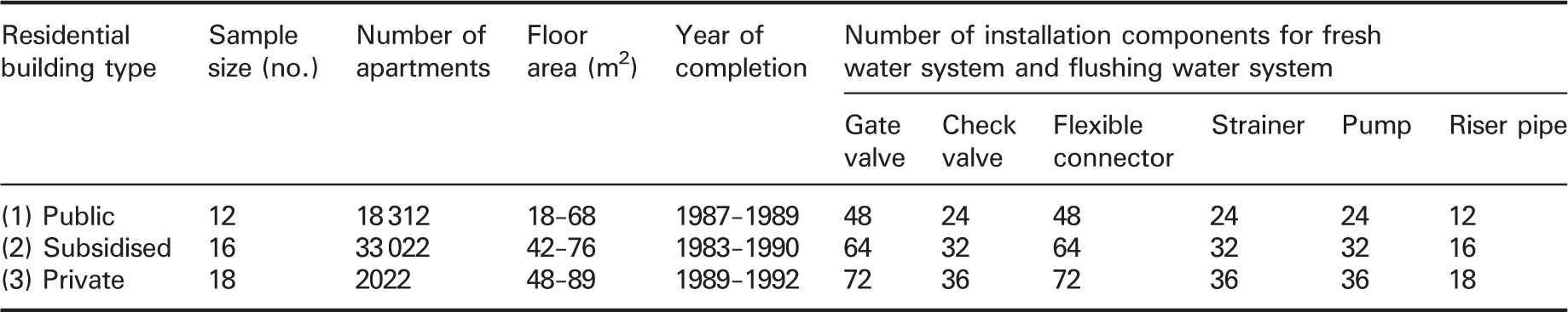
Figure 1 illustrates a typical water pump installation for the surveyed buildings. The installation consists of two gate valves, a strainer, a pump, two flexible connectors, a check valve (non-return valve) and a riser pipe. For three consecutive years (i.e. 2005–2007), failure records of these components including emergency breakdowns and repair times were collected from both of the fresh and flushing water supply systems servicing the buildings. No water pump preventive maintenance was performed in that period.

Figure 1

A typical water pump installation for high-rise residential buildings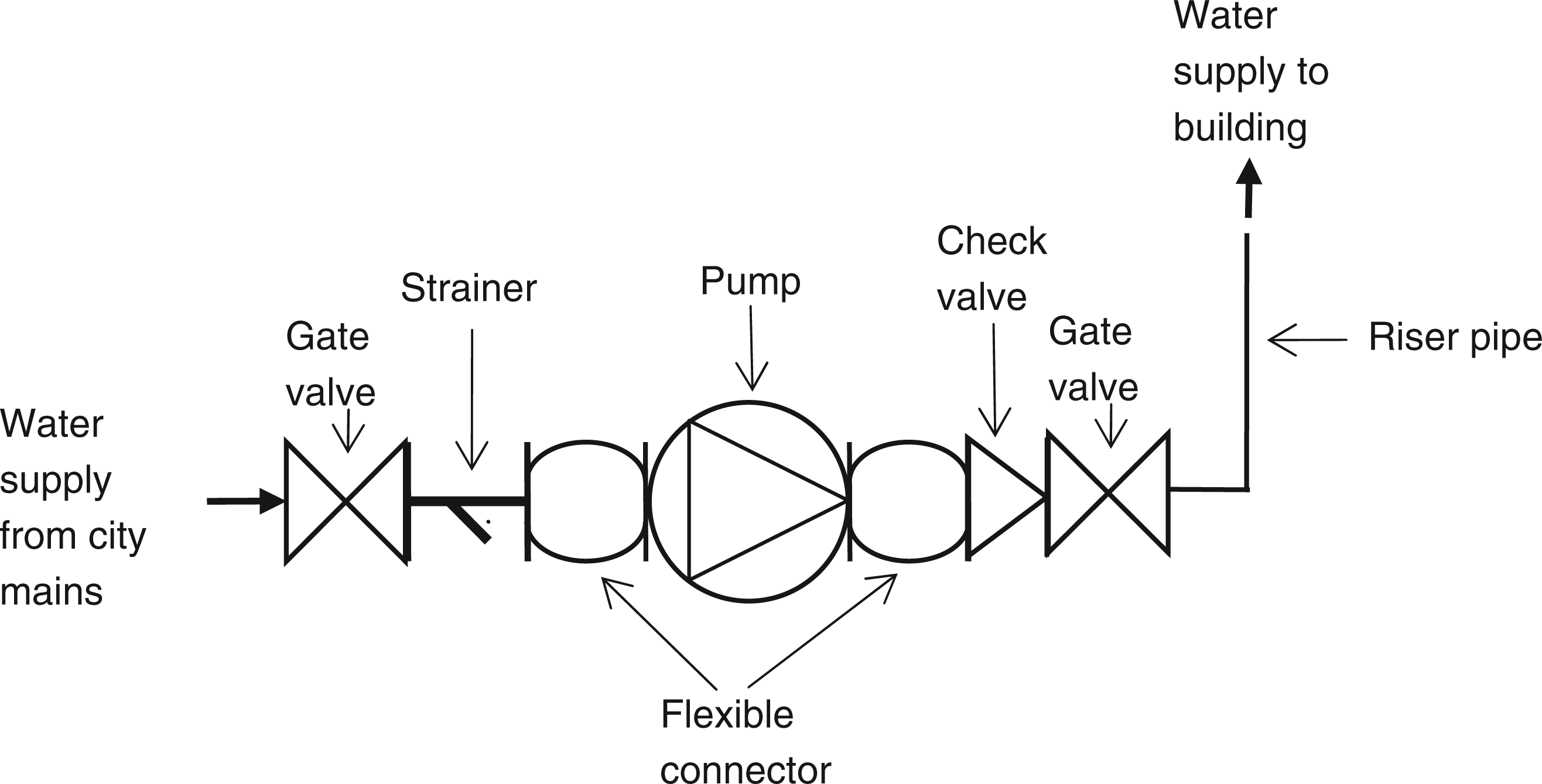

3 Failure records

The total yearly failure counts logged and the restoration times estimated by the component repair engineers are shown in Table 2. For pump failures, two modes are presented – an overhaul needed and a replacement needed. The observed failure rate λ (h⁻¹) can be determined for a component using M, the total number of installation components of the same type and N_f, the total failure counts recorded in the service period τ (=8760 h for 1 year)

(1)

Table 2

Failure records of components in water pump installations

Component	Restoration time (h)	Yearly failure counts N_f for building types (1), (2) and (3)^a									Observed failure rate λ for 3 consecutive years (×10⁻⁶ h⁻¹)					Reference failure rate⁵ λ₀ (×10⁻⁶ h⁻¹)	Component failure rate λ₁ (×10⁻⁶ h⁻¹)
		(1)	(1)	(1)	(2)	(2)	(2)	(3)	(3)	(3)	(1)	(2)	(3)	GM	GSD		GM	GSD
Fresh water system
Gate valve	1–3	0	0	0	0	0	0	0	0	0	0	0	0	–	–	0.1–50	0.02	1.28
Check valve	1–3	0	1	0	2	0	2	1	2	1	4.8	7.1	4.2	5.0	1.5	1–8	5	1.5
Flexible connector	1–3	1	0	1	3	3	9	5	3	2	1.6	8.9	5.3	4.9	1.9	–	4.9	1.9
Strainer	1–3	0	0	0	0	0	0	0	0	0	0	0	0	–	–	–	0.04	2.38
Pump^b	24–72	2	4	4	5	7	3	2	5	2	16	18	9.5	13	1.7	0.7–200	13	1.7
	(12–48)	(1)	(0)	(0)	(2)	(0)	(0)	(0)	(1)	(0)	(4.8)	(7.1)	(3.2)	(4.8)	(1.5)		(4.8)	(1.5)
Riser pipe	1–3	3	3	4	7	2	9	2	15	4	32	43	44	33	1.9	0.2	33	1.9
Flushing water system
Gate valve	1–3	4	4	3	0	9	13	8	2	1	8.7	20	5.8	7.9	2.4	0.1–50	7.9	2.4
Check valve	1–3	0	4	3	5	9	5	7	6	3	17	23	17	18	1.4	1–8	18	1.4
Flexible connector	1–3	2	10	5	0	2	1	0	1	1	13	2.7	1.6	4.2	2.9	–	4.2	2.9
Strainer	1–3	1	1	1	0	5	3	1	1	0	4.8	14	3.2	5.7	1.9	–	5.7	1.9
Pump^b	24–72	6	7	5	3	1	5	9	3	9	29	11	22	17	2.1	0.7–200	17	2.1
	(12–48)	(1)	(2)	(4)	(5)	(11)	(7)	(3)	(13)	(5)	(11)	(27)	(22)	(17)	(2.0)		(17)	(2.0)
Riser pipe	1–3	2	22	88	1	2	5	4	12	8	355	19	51	47	4.3	0.2	47	4.3

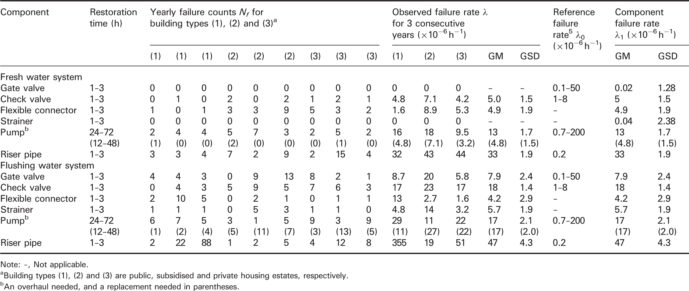
Note: –, Not applicable.

Building types (1), (2) and (3) are public, subsidised and private housing estates, respectively.

An overhaul needed, and a replacement needed in parentheses.

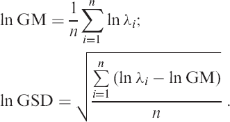
Except for those components that reported zero failures (i.e. the gate valves and strainers in the fresh water system), the geometric mean (GM) and geometric standard deviation (GSD) of λ obtained from the yearly records give the failure rate of a component as follows, where n is the number of yearly records available and i = 1 … n

(2)

According to the literature, water distribution component failure is rarely expected to occur (usually once in >10⁴h of operation).⁵ Apparently, the zero-failure data indicated that a 26 280-h (=3-year) survey was insufficient for accurate analysis. Nevertheless, such data could be employed to improve the state of knowledge of the component failure rate via Bayes’ theorem.⁶

Bayes’ theorem relates the conditional and marginal/prior probabilities of events A and B, where B has a non-vanishing probability. Its key idea is that the probability of an event A given an event B depends not only on the relationship between events A and B but also on the marginal probability of occurrence of each event. For example, if the failure rate of a component determined by a sample test is known to be 99% accurate, it could be due to 1% incorrect identification by the test (false positives), 1% missed cases (false negatives) or a mix of both. The application of Bayes’ theorem allows calculations of the conditional probability of component failure, given an observed failure rate, for any of these three cases.

Hence, for A_i, a set of mutually exclusive and exhaustive events A describing the existing understanding of failure rates i (for i = 1,2, … ) of a specific component, given event B, a new failure-free observation for that component, the posterior probability P(A_i|B) is defined as

(3)

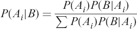
P(B|A_i) can be worked out as follows, where τ is the failure-free service period

(4)

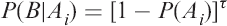
As it was difficult to obtain enough information to determine the precise shape of the failure distribution for the component concerned, a uniform prior probability distribution was assumed for the Bayesian analysis.⁷ Besides, Simpson’s rule was applied to a normally distributed parameter ζ (or its transformation) with mean µ and standard deviation σ as expressed below,⁸ where min, pro and max denote the minimum, probable and maximum values of the parameter ζ

(5)

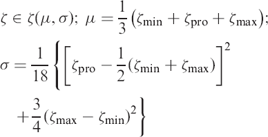
A prior distribution characterised by the GM = 1.2 × 10⁻⁶ and GSD = 35, i.e. λ_a ∼ G(1.2 × 10⁻⁶, 35), as graphed in Figure 2, was suggested in this study. It was decided based on the failure probability range (0.1 × 10⁻⁶ to 15 × 10⁻⁶) reported earlier for other water systems.⁵ Values of P(B|A_i) for the gate valves and strainers where zero failures were observed were determined using Equation (4). Figure 2 also shows the posterior probabilities of these two components given by Equation (3) as the best estimates of the failure rates λ_a_′. The estimates were 0.02 × 10⁻⁶ h⁻¹ and 0.04 × 10⁻⁶ h⁻¹ for the gate valves and strainers, respectively.

Figure 2

Failure rates of gate valves and strainers for fresh water pump installations Note: Posterior estimates for fresh water pump installations. —— Gate valve λ_a′∼G(0.02×10⁻⁶, 1.28); —— Strainer λ_a′∼G(0.04×10⁻⁶, 2.38).

4 Simulations for system failures

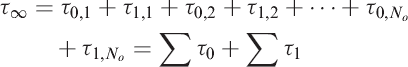
Based on the component failure rates summarised in Table 2, simulations were carried out in order that the failure patterns of both the fresh and flushing water supply systems could be studied. Operation of a pump installation at any time was represented by either ‘state 0’ – installation available or ‘state 1’ – installation failure. Any faulty installation component would lead to state 1 and a downtime τ₁ (h) (i.e. a period of state 1) till the repair was completed. The time between failures was defined as τ₀ (h) (i.e. a period of state 0). Hence, the entire operation period of a pump installation τ_∞ (h) can be expressed by a sum of time series τ_i, where i = 1,2, … , N_o and N_o is the total number of time periods of faulty-available pairs for the installation

(6)

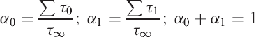
Installation availability α₀ and installation unavailability α₁ are then given by

(7)

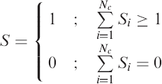
Making use of the non-constant component failure rates from Table 2, operations of a system composed of N_c components connected in series can be approximated via Monte Carlo simulations.

The component operation state S (in each hour) is described by

(8)

where S_i is the operation state of a component i

(9)

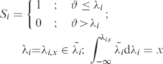
In Equation (9), ${\tilde{λ}}_{i}$ is a distribution function for the component failure rate λ_i at percentile x = ϑ, and ϑ ∈ [0,1] is a random number taken from a pseudorandom number set generated by the prime modulus multiplicative linear congruential generator.⁹ The pseudoset has been tested and applied in a number of engineering applications.¹⁰^–¹²

In this study, a 10-year (i.e. τ_∞ = 87 600 h) operation of 200 water pump installations – 100 fresh and 100 flushing – was simulated. The choice of the simulation period should be long enough to tentatively include more than five expected failure counts per installation component. An expression of the mean time to failure τ_m (h) given by a constant hazard rate model with an assumed exponential time to failure for each component i can be employed to justify the choice¹³

(10)

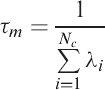
As Equation (10) gave an estimated mean time to failure of 15 316 h (1.7 years) for the fresh water pump installations or 7765 h (0.9 years) for the flushing ones, i.e. an equivalence of six or more expected failure counts within 10 years per installation component, the simulation period was considered satisfactory.

Limited by the computer memory, the number of simulations required had to be balanced by accuracy and simulation run time. Parameter sensitivity to the number of simulations was examined by doubling the number of installations from 100 to 200 and the simulation time from 50 to 100 h per case. As the average values of the parameters concerned (such as τ₀ and τ₁) did not change significantly (p > 0.4, t-test), the simulations of 100 installations for each water supply system were selected for demonstrations.

With reference to some relevant literature, convenient parametric distributions including exponential, normal and Gamma distributions were chosen to fit the simulated data sets of downtime and time between failures in this pilot study.¹⁴^–¹⁸ The exponential probability distribution to which typical equipment failure patterns approximated well would best describe the time between failures for the water pumps.¹⁵ The Gamma distribution, on the other hand, was employed to represent the downtimes for the monotone systems (i.e. systems of only two states: ‘operating’ and ‘failed’) studied.¹⁶ The normal distribution (that is supposed to arise from additive effects of a large number of independent causative random variables) was used to approximate the random outcome.¹⁴ It should be noted that the downtime distribution of a monotone system (either Poisson or Gamma) can be approximated by the normal distribution.^17,18

The counts of τ₀ (h) and τ₁ (h) were obtained from the simulated time series of S. Figure 3 exhibits the counts of τ₀ (h) for both the fresh and flushing water pump installations. τ₀ (h) can be described by exponential distributions (p ≥ 0.5, Chi-squared test) with a density function stated below, where the regression constant ν₀ is 377 (or 0.46 with respect to percentage frequency) for the fresh water pump installations and 2641 (or 1.43 with respect to percentage frequency) for the flushing water pump installations

(11)

Figure 3

Times between failures for fresh and flushing water pump installations Note: ^—— Fresh water pump installations (ν₀, ν)=(377, 92×10⁻⁶); ♦––– Flushing water pump installations (ν₀, ν)=(2641, 247×10⁻⁶).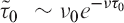

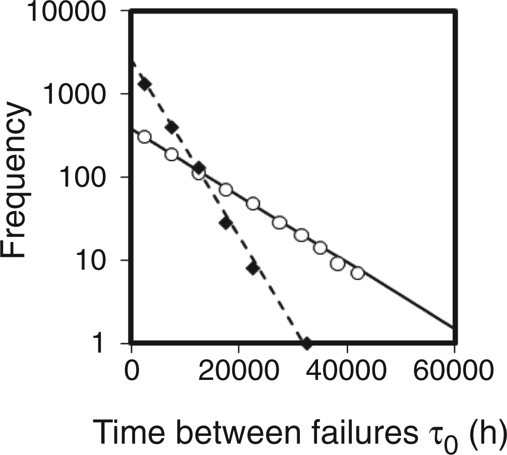
The explanatory parameter values reported for the fresh and flushing water pump installations were ν = 92 × 10⁻⁶ and 247 × 10⁻⁶ corresponding to the mean times to failure τ_m = 10 817 h (1.24 years) and 4048 h (0.46 years), respectively, i.e. about 30% and 50% lower than those estimated using the constant hazard rate model.

Figure 4 shows the downtimes τ₁ (h) for the fresh and flushing water pump installations in terms of frequency and percentage frequency. The failure counts observed in the flushing system were about three times higher and that was consistent with the shorter estimates of mean time to failure found for the system. Most failures (73% and 82% for the fresh and flushing water pump installations, respectively) were in the downtime range from 1 to 5 h; the rest (i.e. 27% and 18%, respectively) had downtimes ≥13 h. Over the 10-year simulation period, the total downtime for the 100 fresh water pump installations was 8990 h with 709 failures and that for the 100 flushing water pump installations was 18 988 h with 2081 failures.

Figure 4

Downtimes of fresh and flushing water pump installations: (a) frequency, (b) percentage frequency Note: —— Fresh water pump installations; ––– Flushing water pump installations.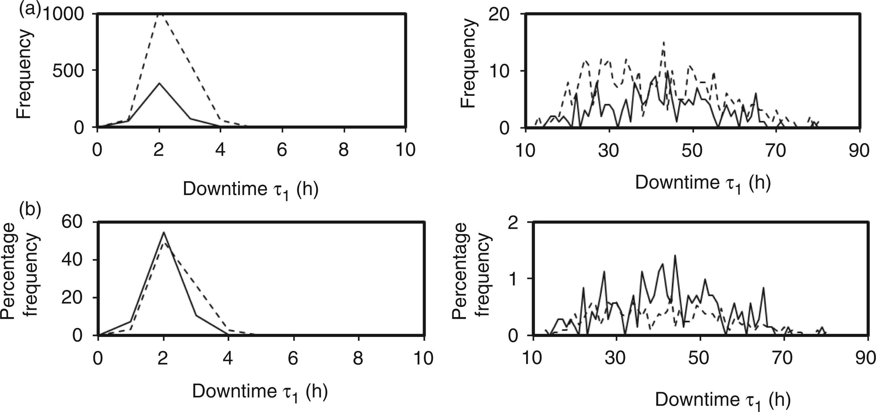

Figure 5 illustrates the downtimes for 100 fresh water supply systems and 100 flushing water supply systems which could be approximated by normal distributions (p ≥ 0.95, Shapiro–Wilk’s test). The average downtime and the corresponding availability for the fresh water supply system were 90 h (SD = 63 h) and 0.90 while those for the flushing system were 190 h (SD = 75 h) and 0.78, respectively.

Figure 5

Downtime of water pump installations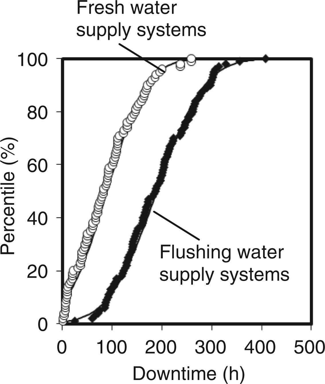

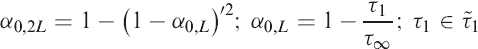
To reduce installation unavailability, pumps are typically operated in parallel (i.e. two installations connected in parallel) as a means of flow control and for emergency back-up. The availability of a parallel pump installation α_0,2 _L is calculated using the following equation, where α_0, _L is the availability of a pump installation,¹⁹ and the downtime τ₁ of each installation can be sampled from the parametric distributions shown in Figure 5 via Monte Carlo simulation

(12)

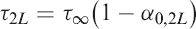
The total downtime of a parallel pump installation τ₂ _L (h) in an operation period τ_∞ (h) is

(13)

It can be approximated by a Gamma distribution (p > 0.95, Chi-squared test), 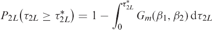${\tilde{τ}}_{2 L} ~ G_{m} (β_{1}, β_{2})$ , for describing the performance in terms of the allowable downtime of the water pump installations. The probability of a parallel pump installation P₂ _L associated with a total downtime τ_2L ≥ $τ_{2 L}^{*}$ (h) in τ_∞ (h) can be determined by

(14)

Figure 6 shows the total downtime distribution of parallel water pump installations. If the maximum allowable downtime per year = 1 h, then P₂ _L would be 40 × 10⁻⁶ and 0.01, respectively for the fresh and flushing water pump installations in Hong Kong residential buildings.

Figure 6

Total downtimes of parallel water pump installations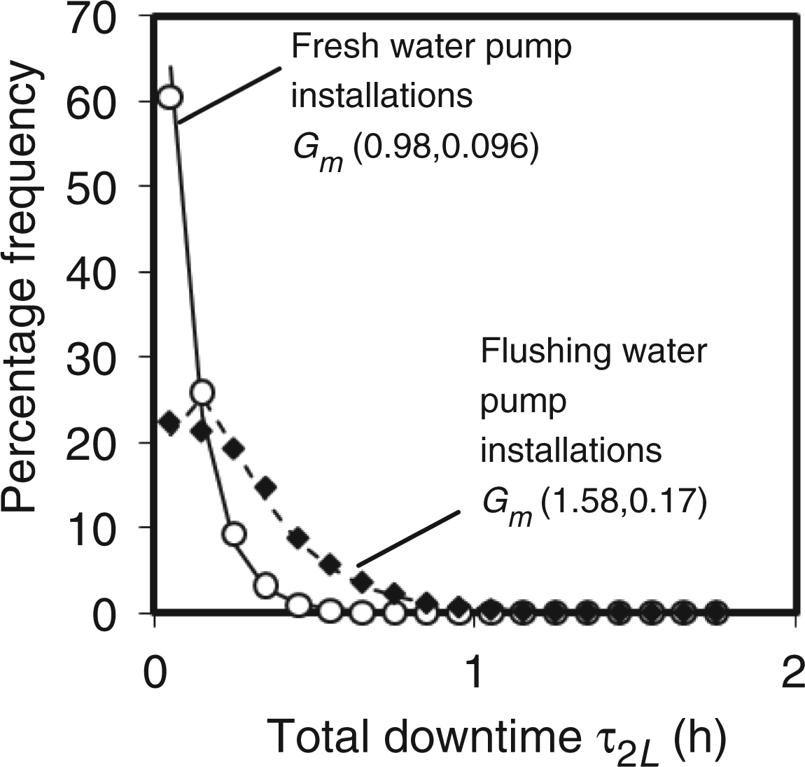

5 Conclusion

Currently in Hong Kong, systematic considerations for the influence of various installation arrangements and usage patterns on the reliability of a water supply system are lacking. Together with some reliability data published elsewhere, this study applied Bayesian analysis to improve our understanding of the downtime characteristics of water pump installations. Based on a survey on water pump failures conducted in Hong Kong from 2005 to 2007 for typical high-rise residential buildings, the failure patterns of installation components were estimated via Monte Carlo simulations. From the virtual operations of 100 parallel pump sets over a period of 10 years, the mean time to failure, total downtime, failure counts and system availability for the fresh water pump installations were 1.24 years, 8990 h, 709 and 90%, while those for the flushing water pump installations were 0.46 years, 18 988 h, 2081 and 78%, respectively. It is noted that for Hong Kong, the seawater flushing water closet is considered as a cost-effective and environment-friendly water conservation measure. This study reported that seawater flushing water pumps were associated with more failures but shorter downtimes than the fresh water supply pumps. The results would be useful in the calculation of water supply availability for high-rise residential buildings while keeping the balance between maintenance cost and system reliability. This study also demonstrated a method for reliability modelling of water supply for high-rise residential buildings.

Footnotes

Nomenclature

Greek

Subscripts

Superscripts

Acknowledgement

The study described in this article was partly funded by the Research Grants Council of the Hong Kong Special Administrative Region, China (PolyU533709E).

References

Lee

. Conservation of water resources – use of sea water for flushing in Hong Kong. Journal of Water Supply Research and Technology-Aqua 1997; 46(4): 202–9.

Luk

Tang

. Sustainability of toilet flushing water supply in Hong Kong. Water and Environment Journal 2005; 19(2): 85–90.

Tao Z. Application of GIS and CARE-W systems on water distribution networks, Skärholmen. Stockholm, Sweden. MSc Thesis, 781027-A242, International Master Programme of Environmental Engineering & Sustainable Infrastructure, Sweden: Kungliga Tekniska Högskolan (Royal Institute of Technology), 2006.

Wong

Mui

. An occupant load survey for residential buildings in Hong Kong. International Journal for Housing Science and its Applications 2006; 30(3): 195–204.

Fong

. Reliability study on sprinkler system to be installed in old high-rise buildings. International Journal on Engineering Performance-Based Fire Codes 2000; 2(2): 61–7.

Gelman A, Carlin JB, Stern HS, Rubin DB. Bayesian data analysis, 2nd edn. Boca Raton: Chapman & Hall/CRC, 2003.

Aitken CGG, Taroni F. Statistics and the evaluation of evidence for forensic scientists, 2nd edn. England: John Wiley & Sons, 2004.

Lerche I, Paleologos EK. Environmental risk analysis, New York: McGraw-Hill, 2001.

Park

Miller

. Random number generators: good ones are hard to find. Communications of the ACM 1988; 31(10): 1192–201.

10.

Wong

Mui

. A transient ventilation demand model for air-conditioned offices. Applied Energy 2008; 85(7): 545–54.

11.

Wong

Mui

. Stochastic modelling of water demand by domestic washrooms in residential tower blocks. Water and Environment Journal 2008; 22(2): 125–30.

12.

Wong

Mui

Guan

. Shower water heat recovery in high-rise residential buildings of Hong Kong. Applied Energy 2010; 87(2): 703–9.

13.

Modarres M, Joglar-Billoch F. Reliability. The SFPE handbook of fire protection engineering, 3rd edn. Section 5, Chapter 3. Bethesda, MD, USA: Maryland, USA: Society of Fire Protection Engineers, JR Hall (Ed.), JM Watts (Ed.), 2002: 24–39.

14.

Jardine AKS, Tsang AHC. Maintenance, replacement, and reliability. London: CRC Press, 2006.

15.

Wagner

Shamir

. Water distribution reliability: simulation methods. Journal of Water Resources Planning and Management 1988; 114(3): 276–94.

16.

Law AM, Kelton. Simulation modeling and analysis, 2nd edn. New York, NY: McGraw-Hill, 1990.

17.

Muth

. A method for predicting system downtime. IEEE Transactions on Reliability 1968; R17(2): 97–102.

18.

Haukas

Aven

. Formulae for the downtime distribution of a monotone system observed in a time interval. Reliability Engineering and System Safety 1996; 52(1): 19–26.

19.

. A study on the reliability of fire water supply system in high-rise buildings. Fire Technology 2002; 38(1): 71–9.