Methodologies for the generation of design summer years for building energy simulation using UKCP09 probabilistic climate projections

Abstract

Design summer years representing near-extreme hot summers have been used in the United Kingdom for the evaluation of thermal comfort and overheating risk. The years have been selected from measured weather data basically representative of an assumed stationary climate. Recent developments have made available ‘morphed’ equivalents of these years by shifting and stretching the measured variables using change factors produced by the UKCIP02 climate projections. The release of the latest, probabilistic, climate projections of UKCP09 together with the availability of a weather generator that can produce plausible daily or hourly sequences of weather variables has opened up the opportunity for generating new design summer years which can be used in risk-based decision-making. There are many possible methods for the production of design summer years from UKCP09 output: in this article, the original concept of the design summer year is largely retained, but a number of alternative methodologies for generating the years are explored. An alternative, more robust measure of warmth (weighted cooling degree hours) is also employed. It is demonstrated that the UKCP09 weather generator is capable of producing years for the baseline period, which are comparable with those in current use. Four methodologies for the generation of future years are described, and their output related to the future (deterministic) years that are currently available. It is concluded that, in general, years produced from the UKCP09 projections are warmer than those generated previously.

Practical applications: The methodologies described in this article will facilitate designers who have access to the output of the UKCP09 weather generator (WG) to generate Design Summer Year hourly files tailored to their needs. The files produced will differ according to the methodology selected, in addition to location, emissions scenario and timeslice.

1 Introduction

The design summer year (DSY)¹ was developed in the United Kingdom as a means of assessing the overheating risk in naturally ventilated and, to a lesser extent, mixed-mode buildings. The DSY is a complete historical year intended to represent near-extreme hot conditions and generally has a return period of approximately 8 years.

Reference years are highly dependent on data availability and, being related to a standard meteorological period (ideally 30 years), represent an assumed stationary climate. The limitations of stationarity have recently become apparent as the life span of new buildings is comparable to the time horizon of contemporary climate models, hence such a building is expected to experience a significant change in climate over its lifetime. The availability of output from general and regional circulation models has opened up the possibility of estimating the future performance of buildings under a range of possible future climates driven by different emission scenarios.

The production of future hourly weather files, by temporal downscaling of climate model output, is problematical. One effective solution is the ‘morphing’ approach where weather variables in existing reference years are shifted and stretched (on a monthly basis) using the climate model output.² Morphed weather years have been used to explore the future performance of a variety of building types in the United Kingdom³ and worldwide.⁴ They are also available commercially for 14 locations in the United Kingdom.^5,6

The recently released UKCP09 climate projections⁷ provide a probabilistic picture of key climate variables, hence they open up the possibility of providing probabilistic reference years which could inform risk-based decision-making. The issues involved in revising the way in which future building simulation weather files are produced are worthy of investigation, as it is likely that the trend towards ensemble climate model runs is likely to increase in recognition of a need for a probabilistic view of future changes.⁸

The morphing methodology enables the temporal downscaling of climate model output by transforming existing reference years, which are based on measured values. This methodology means that the temporal variability of the years is fixed in all future projections. An alternative approach is now available due to the coupling of a statistical WG with the UKCP09 projections.⁹ This produces statistically coherent weather years at daily or hourly resolution, but it should be remembered that the statistical relationships between the variables is determined by analysis of measured data.

A standard run of the generator (WG), for hourly data, produces 100 files, each of which is calculated using change factors sampled from the available range of 10 000 possibilities. Each one of these files can be regarded as representative of a candidate future climate. The files themselves contain a 30-year sequence which encapsulates the inter-annual variability to be expected of a stationary climate. These ‘scenario’ files are accompanied on a one-to-one basis by ‘control’ files which represent the baseline period 1961–1990.

2 Design summer years

2.1 Selection methodology

The current selection process is to assemble measured data for the reference period at the required location, rank the years according to a measure of summer warmth, then select the year corresponding to the middle of the upper quartile of the ranked list.¹⁰ The warmth measure adopted was the average air temperature for the period April–September. This has the merit of simplicity, but it has known problems. In particular, for some locations the level of predicted overheating risk can be greater when using a test reference year (TRY) than the DSY. This clearly conflicts with the concept of the TRY as representative of average conditions and the DSY as near–extreme. Notwithstanding these problems, the view was taken that it would not be appropriate to revisit the DSY concept at this stage, as this would raise substantive issues of accreditation. There is a significant issue with regard to using the DSY in demonstrating compliance with regulations, but we would regard this as a separate issue. The original intention was to facilitate the exploration of building performance under summer conditions and in this context the idea of using a complete year is still valid.

The use of WG output as the resource from which to generate DSYs raises a number of issues. Firstly, there are very large numbers of candidate years from which to select a DSY, in contrast to the limited availability of observed data. Secondly, there are a number of variables which are required by most weather file formats that are not available from the WG, notably wind speed, wind direction, cloud cover and barometric pressure. Some of these quantities are important drivers of building thermal behaviour, particularly, in regard to passive aspects such as natural ventilation and night cooling. Algorithms for accommodating this restriction have been described elsewhere,¹¹ but it is currently an unresolved question as to whether or not these algorithms will be perceived with the same confidence as the measured data which underpins the morphing procedure.

It was decided at the outset to retain the concept of using complete years, as opposed to generating composite years from individual months (an alternative approach adopted by the PROCLIMATION project).¹² This was partly because the re-definition of the DSY concept has wider implications than the scope of this work, but most importantly the retention of complete years means that the statistical methods such as extreme value analysis (for example, the prediction of return periods) can be used to inform risk-based decision-making.

Four methods for selecting a DSY from WG runs were investigated. A flow diagram for the selection methodologies is shown in Figure 1. In a standard WG run, 100 sets of change factors are selected from the 10 000 available. This selection can either be made at random or close to a fixed percentile of one or two change factors (temperature was used here). Percentile sampling means that the probabilistic attribute of the DSY can be established at the outset, but if a range of probabilistic years is required then multiple runs of the WG will be needed.

Figure 1

Flow diagram for design summer year (DSY) methods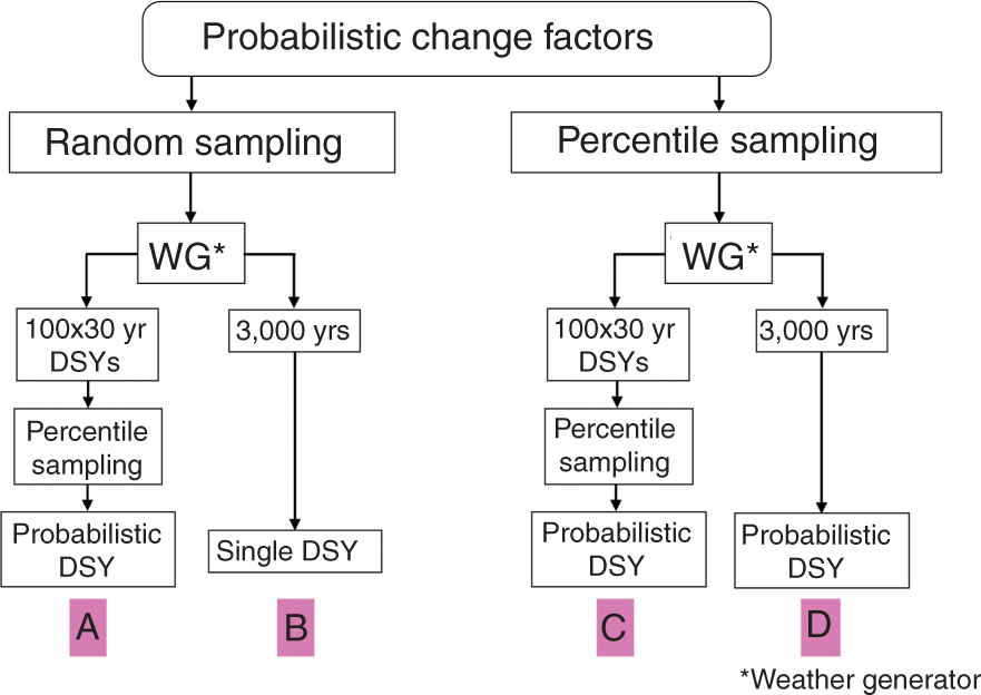

Whichever sampling method is used in the initial stage, there are two possible ways of treating the outputs of a standard WG run. The more logical method is to select one DSY from each of the 100 candidate ‘climates’, which can be regarded as being of equal probability of occurrence. This means that, as at present, the DSYs are selected from within the inter-annual variability of a stationary climate and the distinction between this source of variability and the modelling uncertainty is maintained. If this is carried out following random sampling, then the 100 candidate DSYs can be ranked and a probabilistic DSY obtained by sampling from the ranked list at the required percentile (Method A in Figure 1). If the probabilistic element results from sampling the change factors, selection from the ranked list was made at either the 50% level or the candidate year closest to that with the most probable value was chosen (Method C).

The alternative is to disregard this distinction and to treat all 3000 yearly files as members of the same set. Following random change factor sampling, this results in the determination of the year closest to the mid-point of the upper quartile taking place at the end of the process, hence only one DSY is obtained (Method B). A similar consideration applies if the sampling of the change factors is from a specified percentile; although only one DSY is obtained, it is probabilistic as a result of the initial sampling method (Method D).

2.2 DSYs for the current period

A first step was to compare DSYs produced from the output of the WG for the control period (1961–1990) with the equivalent years from observed data, in order to provide confidence in the generation of future years. This was done for the cities of London, Manchester and Edinburgh¹ as these DSYs (released in 2002) used data closer to the control period than is the case for more recently published data, 1976–1995, 1982–1994 and 1976–1992, respectively. As there are no change factors involved, the DSYs were obtained from the WG by ranking all 3000 control files and selecting the year corresponding to the middle of the upper quartile (Method B in Figure 1). Figure 2 shows that the WG is able to produce DSYs close to those derived from measured data, based on the April–September mean temperature. All three generated DSYs were within 0.5°C of the values derived from observed data.

Figure 2

Comparison of design summer years (DSYs) from the weather generator and from actual years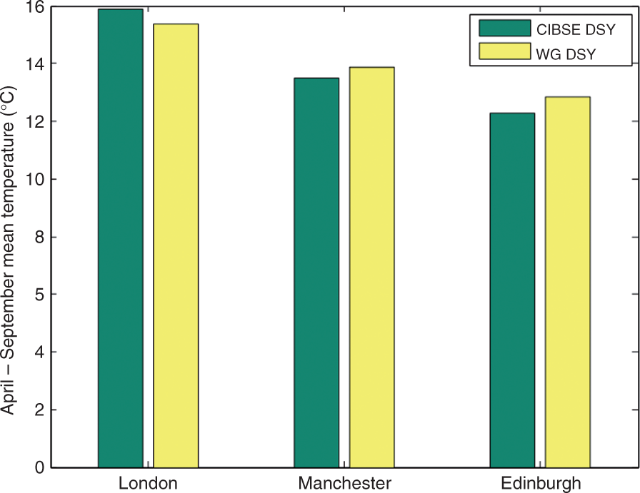

The WG was effective in reproducing the overall temperature statistics for the control period as illustrated in Table 1 for the annual mean temperature (AnMean), April to September mean (A-Smean), July to August mean (J-Amean) and maximum hourly temperature (maxTmax).

Table 1

Temperature-based warmth criteria for London

Data source	AnMean	A-Smean	J-Amean	MaxTmax
BADC data¹³	10.6	14.5	16.9	30.0
Weather generator	10.6	14.6	17.1	29.9

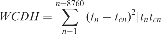
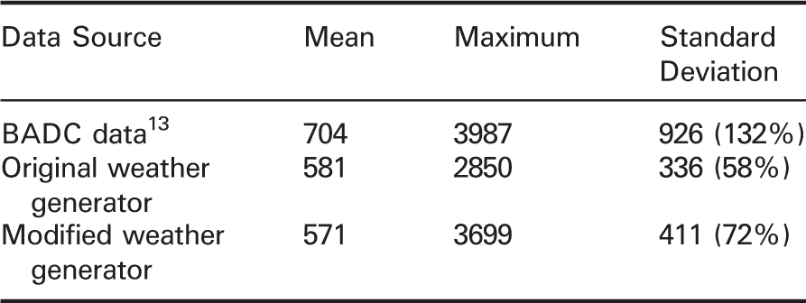
A further method of estimating summer warmth was also used; weighted cooling degree hours (WCDH).¹⁴ This measure is based on the adaptive comfort temperature¹⁵ hence is well-suited to the type of building to which the DSY concept applies.where t_n is the dry bulb temperature at hour n in ^oC and t_c_,_n the corresponding adaptive comfort temperature.

The quadratic nature of this parameter is broadly consistent with the relationship of discomfort with departure from the comfort temperature.¹⁶ In addition, in contrast with measures such as hours over a threshold temperature, it integrates the extent of deviation and therefore better reflects the influence of hot weather periods. The difference in nature of the two measures is illustrated in Figure 3, which illustrates the probability distributions obtained from a WG run for the control period for London. It was found that for both the generated data and the measured data the April to September mean temperature followed a normal distribution, whereas using WCDH generates a Weibull-like distribution. This may impact on the selection of future DSYs as the ‘most likely’ estimate from a Weibull distribution can be different from the central estimate.

Figure 3

Probability distributions for two warmth measures: (a) April to September mean temperature and (b) Weighted cooling degree hours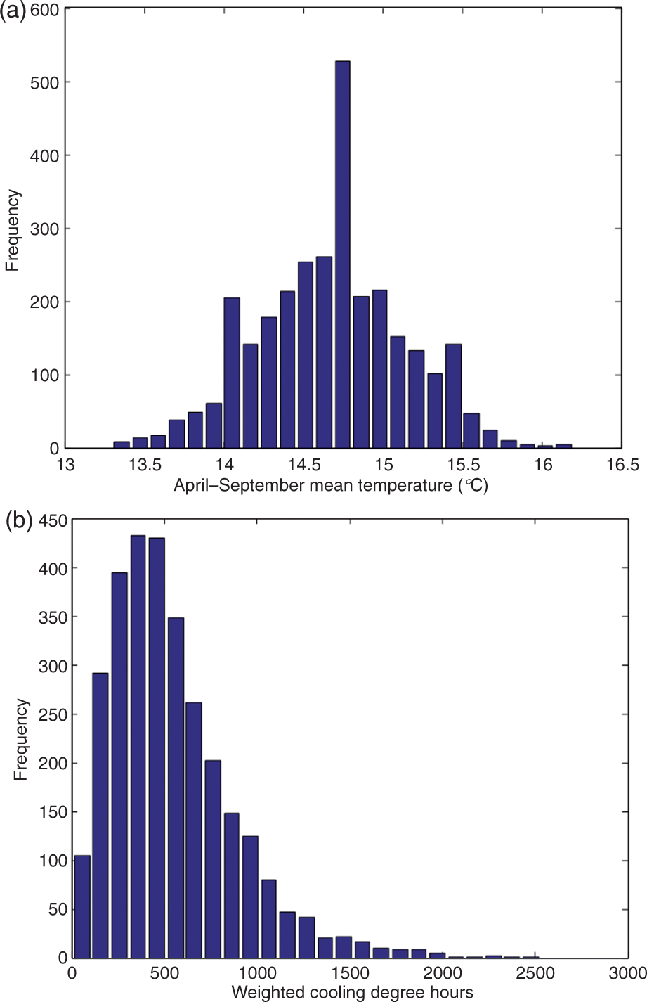

Analysis of WG output indicated that using the WCDH criterion, the generator had limitations in predicting hot spells, as illustrated by the first two rows in Table 2. The hottest observed year (1976) produced a WCDH value of 3987 whereas 3000 runs of the WG produced a hottest year of 2850. Concern over the generation of hot periods led to a modification of the WG,^17,18 which proved much more successful in respect to hot years, as indicated by the last row in Table 2. However, it should be noted that the year-to-year variability of the measured data is still rather higher than that predicted by either version of the WG.

Table 2

Weighted cooling degree hours

Data Source	Mean	Maximum	Standard Deviation
BADC data¹³	704	3987	926 (132%)
Original weather generator	581	2850	336 (58%)
Modified weather generator	571	3699	411 (72%)

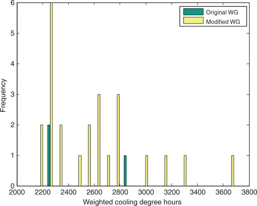
The improved performance is illustrated by the comparison of the probability distributions (for the control period) produced by the two generators as shown in Figure 4. The distributions can be seen to be broadly very similar, but a focus on the warm ‘tail’ of the distribution emphasises the improved performance of the new version in generating hot years (Figure 5).

Figure 4

PDF for the two weather generators - London

Figure 5

Warm tail of the distribution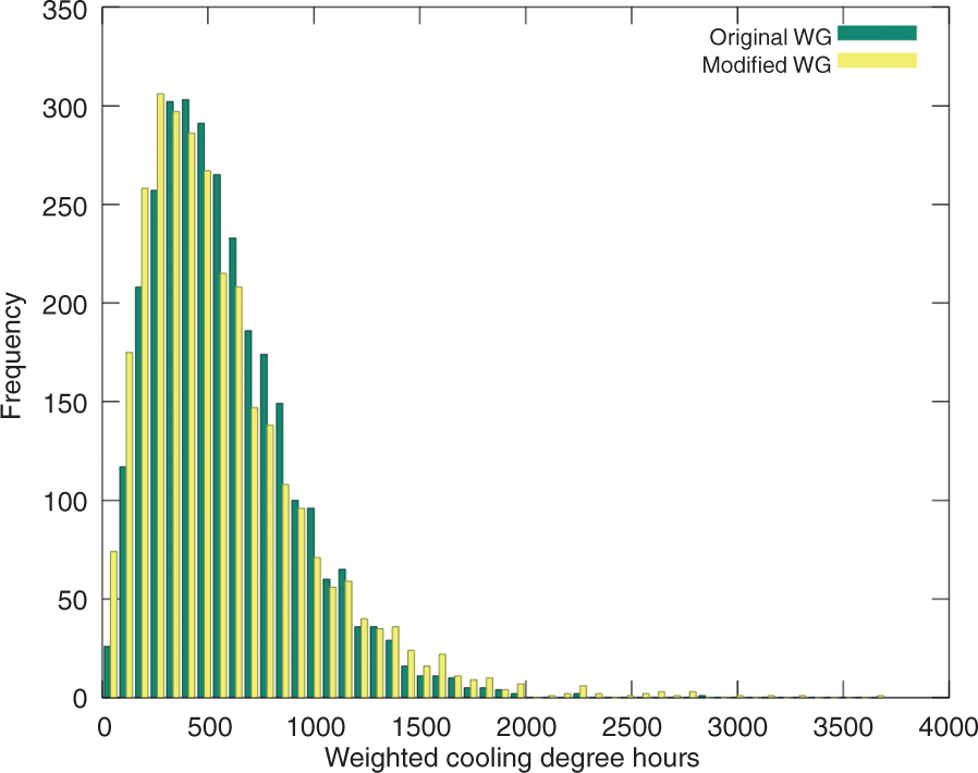

2.3 Characteristics of future DSYs

A framework is needed which can form a basis for comparison of future, probabilistic DSYs. The reference adopted was the existing morphed DSYs obtained from the UKCIP02 projections.⁵ These projections covered the same time span as in UKCP09, but had three timeslices (20s, 50s and 80s) and used four emission scenarios instead of the three used in the most recent projections. The existing DSYs for London are shown in Figure 6.

Figure 6

Morphed design summer years (DSYs) for London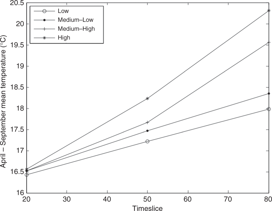

The High and Low scenarios from UKCIP02 are equivalent to those used in UKCP09 so just these two sets of values were used as comparators. Method A represents the closest procedure to that which underpins the selection of the current DSYs, hence by implication the morphed reference years. Operating Method A produces 100 candidate DSYs, each of which represents a plausible future climate. For comparison purposes, these were ranked and a representative year selected at the 50th percentile. Figure 7 shows the results for London, for the two comparable emission scenarios and the three coincident timeslices. In every case, Method A produced slightly warmer DSYs than the morphed versions calculated from UKCIP02 data, a trend that was maintained across all three locations studied. This is consistent with the general observation that UKCP09 projections are somewhat warmer than those from UKCIP02, which may result from some significant advances in climate modelling.¹⁹

Figure 7

Method A design summer years (DSYs) compared to morphed UKCIP02 files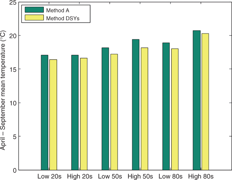

Method B, in which all 3000 files are processed together, was only used in the selection of DSYs from the control runs, as carrying out the DSY selection from all the files produced by a random change factor run precludes obtaining probabilistic reference years.

An important consideration is to ascertain if there is any significant difference between operating the WG such that the change factors are selected on a probabilistic basis (Methods C and D), compared to using randomly selected change factors (Methods A and B) and applying the probabilistic selection later in the process. Method D will produce a single probabilistic year (defined by the change factor selection) whereas Method C produces 100 candidate DSYs. In this case, a single year was selected at the 50th percentile after ranking on the warmth measure. It should be noted that, if probabilistic years are required at, for example, 10th, 50th and 90th percentiles, then these can be obtained from a single WG run using method A, whereas methods C and D required three WG runs.

Figure 8 compares Methods A, B, C and D for London for the 2050s medium emission scenario using the two warmth measures taking the central estimate in each case. Based on April–September mean temperature there appears to be little difference between the three probabilistic methods, but method A (using random change factor sampling) always produces slightly warmer years than the alternative methods. The differences between the methods are amplified if the non-linear WCDH criterion is used.

Figure 8

Probabilistic design summer years (DSYs) for alternative warmth measures: (a) April to September mean temperature and (b) Weighted cooling degree hours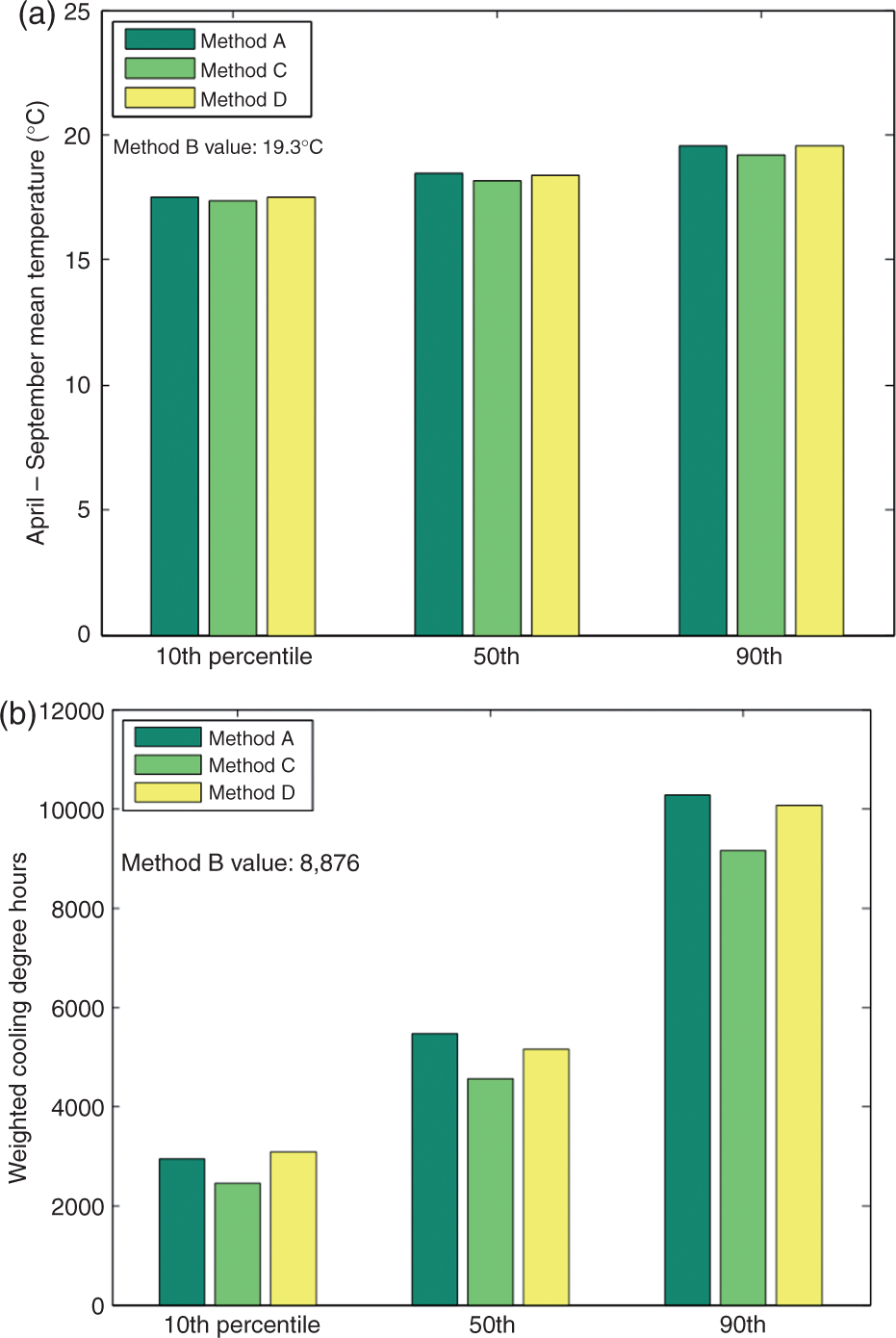

3 Conclusions

Four procedures have been investigated for producing probabilistic future Design Summer Years (DSYs) using the output from the UKCP09 WG. The existing basis for DSY selection was maintained, that is a sequence of candidate years representing a stationary climate are ranked according to a measure of summer warmth and the year at the mid-point of the upper quartile is selected. Whilst this procedure is open to criticism, there has not been any meaningful analysis of alternative procedures; though this is an area of current activity. The ranking used in this work was the mean April– September temperature, as used at present although results from the use of an alternative measure, WCDH, are also presented here. WCDH are shown to provide greater discrimination between candidate years than the existing criterion.

The initial stage was to establish the extent to which output from the WG, using weather files generated for the control period 1961–1990, could produce DSYs comparable to those that were derived from measured data. This was done for three locations: London, Manchester and Edinburgh as the DSYs for these cities were obtained from data most closely aligned with the control period. This comparison showed that the WG aligned well with measured data in generating reference years, thus providing an underpinning of confidence in the projections. In addition, the modifications made to the WG in late 2010 improved significantly its performance in generating hot years such as 1976.

The generation of hourly data files for future timeslices and emission scenarios from the WG was performed in two ways: change factors were either sampled at random or centred around a specified point in the probability distribution of temperature, specifically at the 10, 50 and 90 percentile levels. The latter method has a significantly higher computational overhead in that the WG has to be run for each percentile. The resulting output was typically 100 files, each representing a plausible future climate. Each of these files, in turn, consisted of 30 one-year sequences, thereby encapsulating inter-annual variability. Processing the output in this way maintains a distinction between the two sources of uncertainty.

The alternative treatment is to lose this distinction by treating all 3000 years as members of one set. If this is done using random sampling then it is not possible to generate probabilistic DSYs, as only one year can be selected using the DSY criterion. If the WG output is obtained by sampling from a restricted part of the probability density function of the temperature change factor, then a single probabilistic year is obtained from each WG run.

We maintain that random sampling of the change factors, followed by selecting DSYs from the resulting set of plausible climates (Method A in the text), affords greater flexibility and mirrors the existing selection process more closely than any of the three alternatives. It also allows for greater transparency in that the distribution of the candidate DSYs can be readily ascertained.

Whereas the outputs from the control period could be compared with their equivalents obtained from measured data, this is clearly not possible for future projections. The existing future DSYs, produced by ‘morphing’ existing years using change factors from UKCIP02 data, were used as a framework with which to compare the outputs of the methods investigated which can produce probabilistic years. It is recognised, however, that comparison of UKCIP02 to UKCP09 is complicated by differences in the modelling procedures.

It was shown that, for comparable timeslices and emission scenarios, the central estimates from the probabilistic DSYs were fairly close to those of the existing morphed years. In general, the centrally estimated DSYs produced from the UKCP09 projections were slightly warmer than those derived from UKCIP02, which is to be expected given the general characteristics of the two projections.

In terms of overall performance Method A affords the most flexibility and economy of effort. If its central estimates are used, it provides comparable outputs in relation to the existing morphed methods, and a range of probabilistic years is easily extracted from its output. If such an outcome is needed, then a range of DSYs is easily generated, which can be used to support risk-based decision-making. The methods described here preserve the statistical coherence of individual years, hence can be used with further techniques such as extreme value analysis. Even if probabilistic years are not required, the ability to generate output on a 5-km grid, together with lack of reliance on the availability of measured data, are positive indications that reference years produced by this method offer some advantages over those currently available. However, it remains to be seen whether the algorithms that have been developed to add in the data which are not available directly from the WG will develop sufficient confidence to underpin the industrial uptake of this method of producing probabilistic years.

Footnotes

Figures 1–5, 7 and 8 appear in color online:

Acknowledgement

The authors would like to acknowledge support for the PROCLIMATION project from the Engineering and Physical Sciences Research Council under grant EP/F038151 ‘The use of probabilistic climate change scenarios in building environmental performance simulation’.

References

Chartered Institution of Building Services Engineers (CIBSE). Guide J: weather, solar and illuminance data, London, CIBSE, 2002.

Belcher

Hacker

Powell

. Constructing design weather for future climates. Building Services Engineering Research and Technology 2005; 26: 49–61.

Chartered Institution of Building Services Engineers (CIBSE). Climate change and the indoor environment: impacts and adaptation TM 36, London, CIBSE, 2005.

Crawley

. Estimating the impacts of climate change and urbanization on building performance. Journal of Building Performance Simulation 2008; 1(2): 91–115.

Chartered Institution of Building Services Engineers (CIBSE). CIBSE TRY/DSY hourly weather data set – 14 sites, London, CIBSE, 2009.

Hacker

Capon

Mylona

. Use of climate change scenarios for building simulation: the CIBSE future weather years. The Chartered Institution of Building Services Engineers, London, UK. CIBSE TM48: 2009.

Murphy

Sexton

DMH

Jenkins

Booth

BBB

Brown

Clark

Collins

Harris

Kendon

Betts

Brown

Humphrey

McCarthy

Donald

Stephens

Wallace

Warren

Wilby

Wood

. UK climate projections Science Report: climate change projections, Exeter UK, Met Office Hadley Centre, 2009.

Slingo

Bates

Nikiforakis

Piggott

Roberts

Shaffrey

Stevens

Vidale

Weller

. Developing the next generation climate system models: challenges and achievements. Proceedings of the Royal Society A: Mathematical, Physical and Engineering Sciences 2009; 367: 815–31.

Jones

Kilsby

Harpham

Glenis

Burton

. UK climate projections Science Report: projections of future daily climate for the UK from the weather generator, UK, University of Newcastle, 2009.

10.

Levermore

Parkinson

. Analyses and algorithms for the new test reference years and design summer years for the UK. Building Services Engineering Research and Technology 2006; 27(4): 311–25.

11.

Watkins

Levermore

Parkinson

. Constructing a future weather file for use in building simulation using UKCP09 projections. Building Services Engineering Research and Technology 2011; 32(3): 293–299.

12.

Eames

Kershaw

Coley

. On the creation of future probabilistic design weather years from UKCP09. Building Services Engineering Research and Technology 2011; 32(2): 127–42.

13.

British Atmospheric Data Centre. MIDAS land surface stations data. Available at: www.badc.nerc.ac.uk/ukmo-midas 2006 (accessed 12 May 2011).

14.

Nicol

Hacker

Spires

Davies

. Suggestion for new approach to over-heating diagnostics. Building Research and Information 2009; 374, 348–57.

15.

Humphreys

Nicol

. Understanding the adaptive approach to thermal comfort. ASHRAE Transactions 1998; 104(1): 991–1004.

16.

Nicol

Humphreys

. Adaptive thermal comfort and sustainable thermal standards for buildings. Energy and Buildings 2002; 34: 563–72.

17.

UKCP09. Available at: www.ukclimateprojections.defra.gov.uk/content/view/1206/500/.

18.

Jones

Harpham

. Available at: www.ukcip.org.uk/wordpress/wp-content/UKCP09/UC_2211_CRU.pdf.

19.

UK Climate Projections (UKCP09), DEFRA. Available at: www.ukclimateprojections.defra.gov.uk/content/view/1338/531/.