Freezing soil effects on earth-contact heat transfer

Abstract

The inclusion of soil freezing and snow cover within the context of a building energy simulation is explored. In particular, a method of including soil freezing within the simulation of heat flow from a building to the neighbouring foundation soils is considered. Non-linear thermal conductivity and heat capacity relations are explored that account for the effect of soil freezing. In addition, the work also considers latent heat generated by phase change that occurs as the soil water temperature reduces and ice forms. A simple approach to represent the insulating effect that snow cover may have on the net heat flow at the ground surface is also provided. The approach is illustrated by application to the simulation of a full-scale ground heat transfer experiment performed by others. The results provide a first indication of the potential significance of the inclusion of ground freezing within the context of modelling heat transfer from a full-scale monitored building. Overall transient temperature variations are shown to be dependent on ice content and latent heat effects. Non-linear, ice-content dependent, thermal conductivity and heat capacity are included in the work. Good correlation between measured and simulated temperature variations has been achieved.

Practical application: The principle application relates to the assessment of heat transfer from buildings through to the underlying foundation soils. In addition, the work is of direct relevance to a wider range of applications, for example, ground source heat pumps, thermo-active piles and foundations. The model lends itself to application with respect to utilisation of ground energy within the context of pavement design, particularly, in relation to the alleviation of winter ice problems. It also applies within the context of assessment of urban heat island phenomenon and heat and moisture transfer beneath freezer foundations.

Keywords

Soil freezing thermal simulation heat transfer building energy earth contact

Introduction

The fact that space heating accounts for roughly 60% of total delivered UK residential energy demand underpins the drive towards more sustainable construction and energy utilisation in the future.^1,2 Furthermore, the UK Government’s Climate Change Bill 2008 commits the country to a reduction in carbon dioxide emissions of 80% by 2050 based on 1990 levels.³ Innovation in energy-efficiency and improved uptake of renewable energy technologies can make key contributions in this respect. The role that ground heat transfer can make with respect to these objectives is increasingly recognised. In the building energy sector, ground-coupling has been investigated for a number of years. The specific contribution of heat loss from buildings through foundation materials to the underlying foundation soils has received considerable attention – Zoras⁴ provides a recent review.

Well-established technologies also exist for ground energy utilisation, for example, ground source heat pumps, thermo-active piles and foundations, among others.⁵ Lui et al.⁶ present an in-depth investigation of the role of ground heat transfer within the context of the urban heat island phenomenon. Innovative approaches are now emerging with respect to utilisation of ground energy within the context of pavement design (performance) – particularly, in relation to the alleviation of winter ice problems.⁷ Krarti^8,9 presented research on the assessment of heat and moisture transfer beneath freezer foundations. This work also requires an intimate understanding of the thermo-dynamic response of the underlying soil profile. Overduin et al.¹⁰ presented a detailed study on the measurement of thermal conductivity in freezing and thawing soils. They provide field data collected (in Alaska) from a complete freeze–thaw cycle in silty clay. Their results showed a seasonally bimodal apparent thermal conductivity, with a sharp transition between frozen and thawed values during thaw. The use of soil composition data to account for changes in heat flow due to the effect of latent heat during phase change was used to develop a relationship between soil thermal conductivity and temperature.

In many of the above practical problems, ice formation may contribute to the overall ground energy picture and this fact provides a key motivation for the current paper. In particular, the current work aims to explore the influence of ground freezing on earth-contact heat transfer from a test building. The particular data set studied in this paper has been previously considered by Rees et al.¹¹ who provide some further background on the experimental set-up. Their work focused on the determination of representative initial conditions and demonstrated that some aspects of the problem can be better represented via three-dimensional (3D) simulation. However, their results were described as yielding ‘fair’ correlation to the measured data and highlighted an issue related to the reliability of a section of the boundary data provided in the experimental data set. The simulations presented were based on the solution of the standard heat conduction equation and no attempt was made at that time to consider the possible influence of soil freezing during the winter months.

In view of the above, the current paper re-visits the Minnesota data set^11,12 with the aim of specifically exploring the influence of soil freezing. To this end, an extended theoretical model is presented here that includes ice formation and provides a relatively simple method of estimating the influence of ice content on the key thermal properties of the soil – namely, thermal conductivity and specific heat capacity. Latent heat of fusion associated with the phase change that takes place as water turns to ice and vice versa is explored for the first time within the context of this type of field problem. The current work also includes a correction to the external boundary data that was used previously and an exploration of the impact of snow on the ground surface boundary condition.

Theoretical and numerical model

The approach used in this study to represent heat transfer in a partially saturated frozen soil subjected to freezing conditions is based on a coupled thermo-hydro-mechanical model of frozen soils presented by Thomas et al.¹³ Thomas et al.’s model has been simplified to consider only the thermal field and extended to consider unsaturated conditions; thereby allowing the impact of partially saturated pores on freezing processes to be considered.

In this study, the soil is assumed to be a partially saturated medium within which the soil is fully frozen, partially frozen or unfrozen and considered to consist of solid grains, pore air, pore water and pore ice. Local thermal equilibrium is assumed, that is, the local temperature is the same for soil solid, pore water and ice. The approach developed allows consideration of (a) conduction, (b) phase change of pore water, (c) latent heat of fusion on freezing and thawing, (d) impact of partial saturation and freezing on thermal conductivity and heat capacity, (e) non-linear variation of ice content with temperature and (f) heterogeneous variations in moisture content.

Moisture and ice content

The volumetric moisture content for freezing soils is defined as the sum of the volumetric water content θ _l and the volumetric ice content θ _i , respectively, which are defined as θ _l = n(1 – S_i)S_r and θ _i = nS_iS_r, where n is the porosity of the freezing soil. S_r is the degree of moisture saturation and, in the absence of consideration of moisture movement, is assumed as a heterogeneous constant. S_i refers to the degree of moisture in the ice phase and can be represented by a power function of the temperature according to many experiments with varying water contents and different physical properties¹⁴

S_{i} = 1 - [1 - (T - T_{0})]^{α} T \leq T_{0}

(1)

where T is temperature (in Kelvin or ℃) and T₀ is the freezing point of pore water, α is a parameter which is dependent on pore size, if variations of the chemical composition of the pore liquid are not considered. As this relationship only tends towards unity, a threshold value of S_i is used to indicate a fully frozen state within the model. Figure 1 shows the relationship of S_i and T–T₀ with α ranging from −10 to −1. Alternatively, a linear relationship can be used, with T_s representing the temperature at which the soil is fully frozen, sometimes termed the segregation temperature

S_{i} = \frac{(T_{0} - T)}{(T_{0} - T_{s})} T_{s} \leq T \leq T_{0}

(2)

Figure 1.

Relationship between degree of moisture in the ice phase and temperature (after Thomas et al., 2009).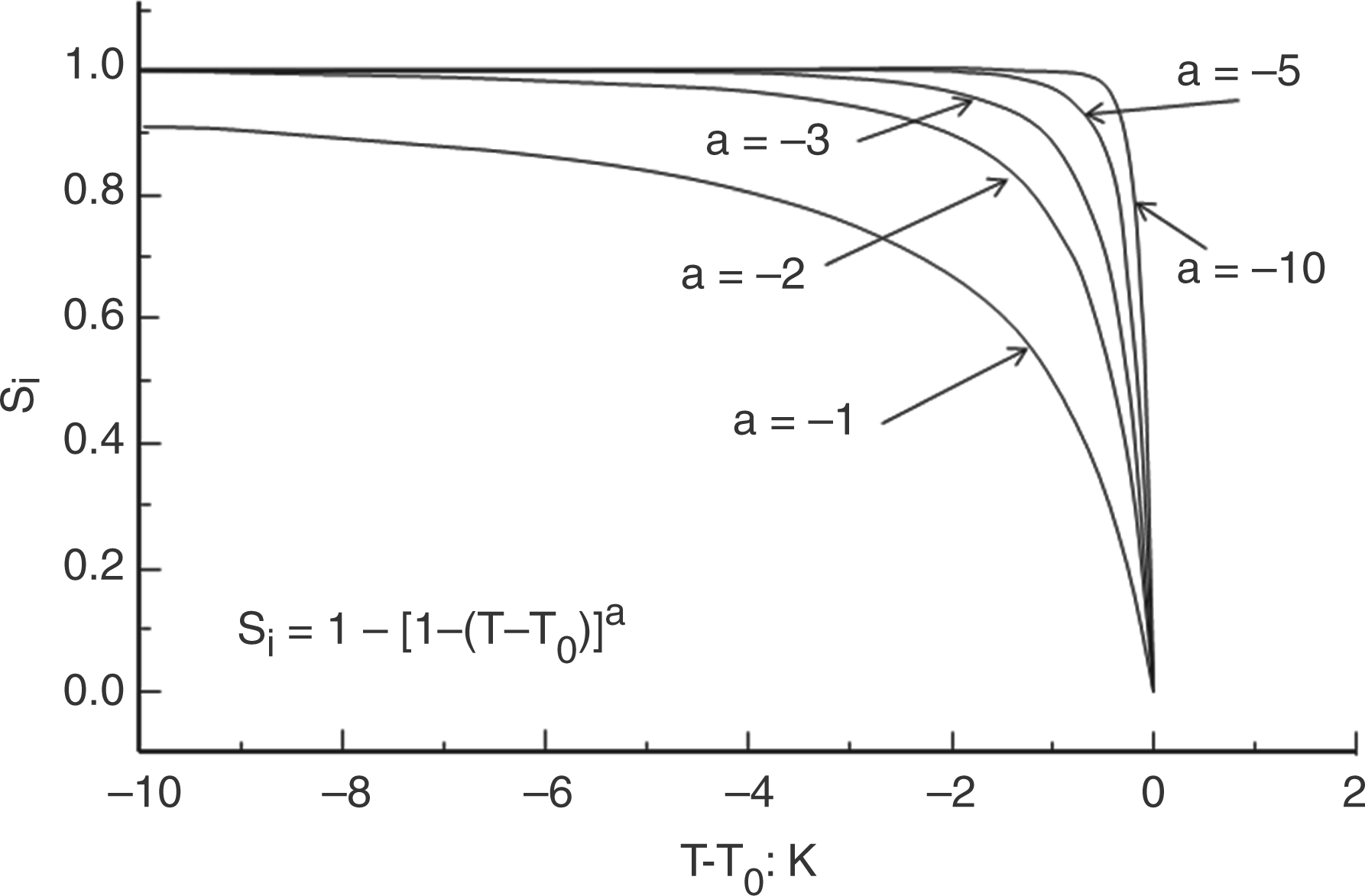

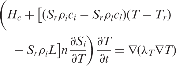
Heat transfer

The law of energy conservation of heat for freezing soils can be expressed as

\frac{\partial (Φ d V)}{\partial t} + \nabla Q d V = 0

(3)

where Φ refers to the heat content of soil per unit volume and is defined as

Φ = H_{c} (T - T_{r}) - {LnS}_{r} S_{i} ρ_{i}

(4)

where T_r is the reference temperature, L is the latent heat of fusion, ρ _i is the density of ice and H_c is the volumetric heat capacity of the soil and is defined, based on De Vries method,¹⁵ as

H_{c} = (1 - S_{i}) S_{r} n ρ_{l} c_{l} + {nS}_{r} S_{i} ρ_{i} c_{i} + n (1 - S_{r}) ρ_{a} c_{a} + (1 - n) ρ_{s} c_{s}

(5)

where c_l, c_i, c_a and c_s are the specific heat capacities of pore water, pore air, pore ice and the solid particles, respectively; ρ _l , ρ _a and ρ _s are the density of pore water, pore air and the solid particles, respectively. Q is the heat flux per unit volume, including conduction and pore water convection and is defined as

Q = - λ_{T} \nabla T

(6)

where λ_T is the thermal conductivity of the soil and will vary with degree of moisture saturation and degree of moisture in the ice phase. Finally, the governing equation of heat transfer can be written as

(H_{c} + [(S_{r} ρ_{i} c_{i} - S_{r} ρ_{l} c_{l}) (T - T_{r}) - S_{r} ρ_{i} L] n \frac{\partial S_{i}}{\partial T}) \frac{\partial T}{\partial t} = \nabla (λ_{T} \nabla T)

(7)

Solution of the governing equation for heat transfer for initial value problems has been achieved by implementation of a Galerkin weighted residual finite element approximation for the spatial terms and a finite difference approximation for the temporal terms. This approach has been shown to provide stable solutions to highly non-linear problems.^16,17

Experimental case study

The framework outlined above is explored by application of the model to the simulation of field-measured data. In particular, the data used was measured at a full-scale experiment carried out at the University of Minnesota, Minneapolis, United States.^11,12 The experimental building was square in plan (5.89 × 5.89 m²) with a wall thickness of 304.8 mm. Figure 2 provides a cross section through the building illustrating the ground conditions salient to the problem considered here. The building was instrumented extensively, both inside (26 internal temperature and heat flux measurement locations) and in the envelope (733 transducer locations). Unfortunately, no measurements in the surrounding ground were made.

Figure 2.

Minnesota experiment (dimensions in mm).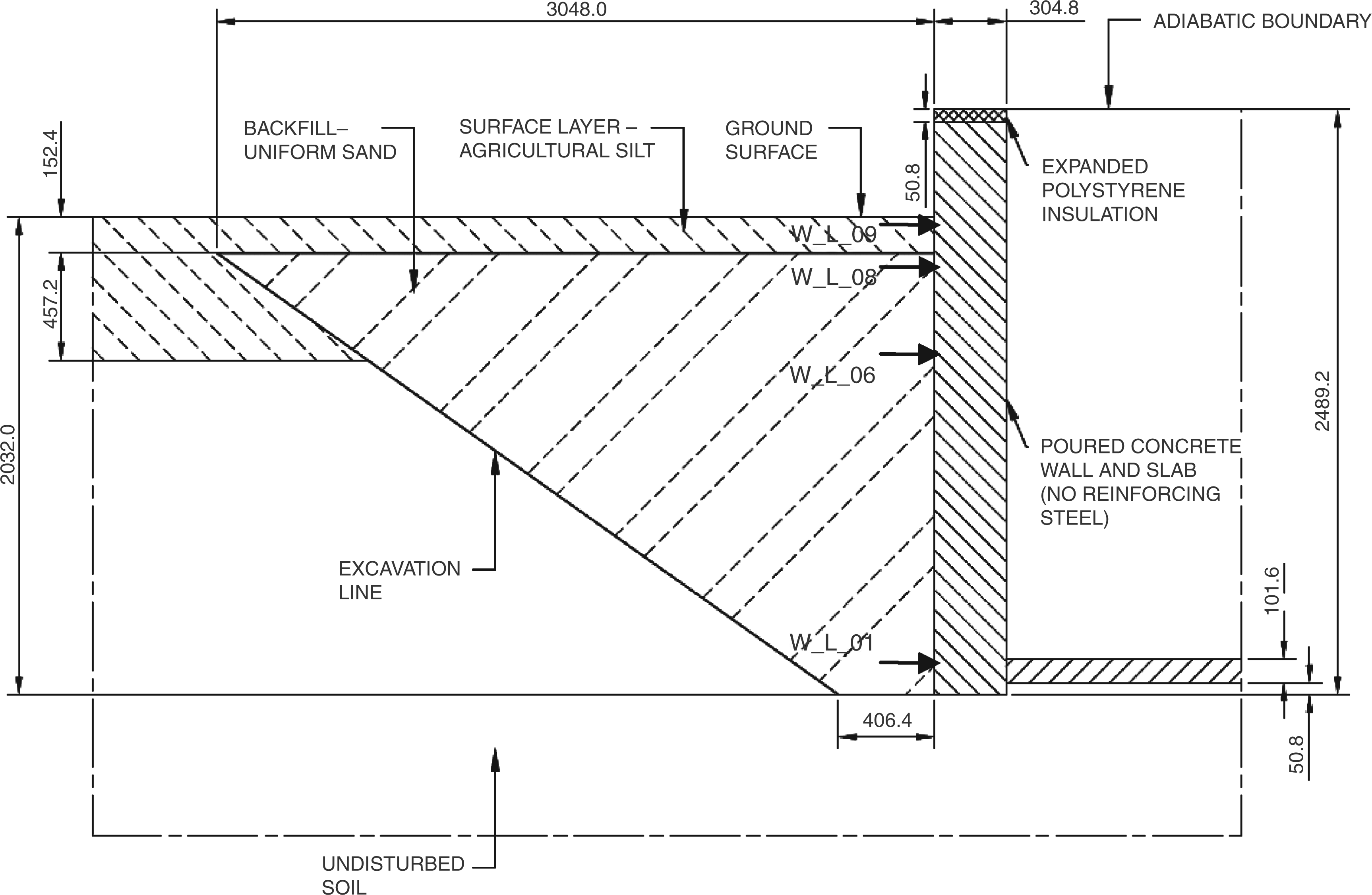

In order to assess the performance of the numerical model, the results from four transducers located in the West wall of the building (as shown in Figure 2) have been considered. These are referred to W_L_01, W_L_06, W_L_08 and W_L_09 located at depths below ground of 1887.5 mm, 661.1 mm, 203.9 mm and 51.5 mm, respectively. W_L_01 is located near the finished floor level of the building and W_L_09 is located near the ground surface. All four transducers were embedded 6.35 mm below the exterior surface of the concrete wall.

The seasonal period under consideration ranges from 1 September 1990 to 30 April 1991 (a total of 243 days). During this period, the main precipitation was in the form of snowfall. A small amount of rainfall occurred in April (approximately 3 mm/day on average over the month). The ground surface was covered with snow for a considerable proportion of the period under consideration. The measured daily mean air temperatures inside and outside (dry-bulb) are presented in Figure 3. The mean indoor air temperature variation is based on an average of four internal surface transducers. As would be expected, the magnitude of variation in external temperature is clearly much greater than that occurring inside the structure.

Figure 3.

Boundary data.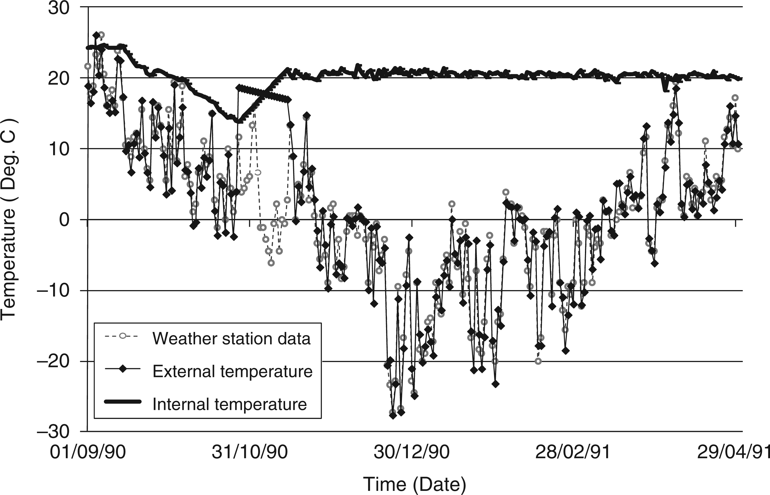

In the raw data presented in Figure 3, it is clear that the external temperature readings failed for the period between18 October 1990 and 13 November 1990 – the plotted data simply shows a linear fit in this region. An attempt has been made to estimate the external temperature during this period using data from a local weather station (Minnesota airport). The data from this station is also provided in Figure 3 for direct comparison with the air temperature data measured at the experimental site for the whole time period considered. The overall pattern of behaviour appears similar in both locations. Statistical analysis between the two data sets (excluding the period between 18 October 1990 and 13 November 1990) yields a root mean square error (RMSE) value of 1.79℃. Therefore the data provided at the local airport weather station has been used to ‘correct’ the faulty patch of data recorded at the experimental site. In addition, an indication of the depth of snow cover during the period of the experiment was obtained from the State Climatology Office in University of Minnesota, St. Pauls (Minnesota, USA). This information indicated that the ground surface was covered with snow for considerable periods, particularly, in December 1990 and January 1991. Figure 4 presents the ‘corrected’ external air temperature along with the approximate depth of snow cover.

Figure 4.

Boundary data (corrected) and snow depth.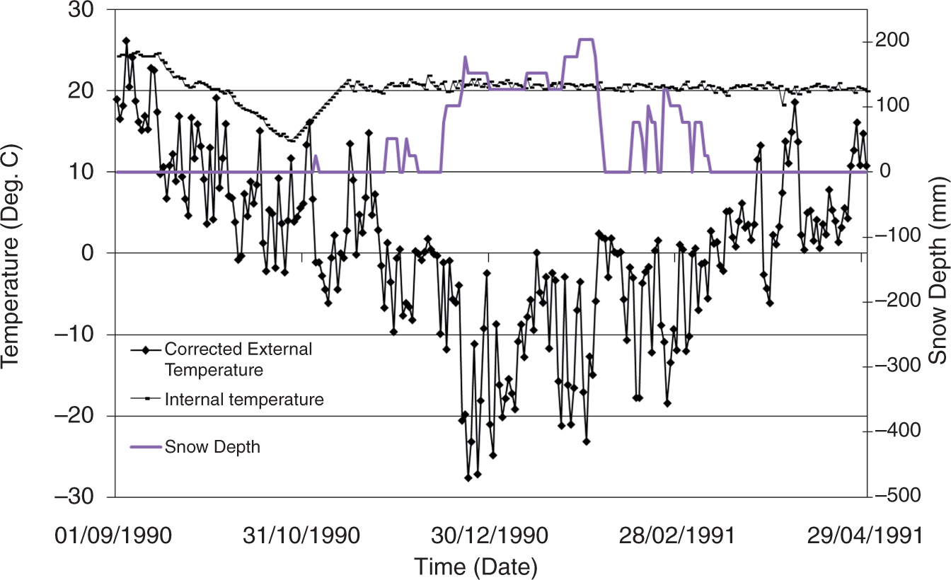

No transducers were located in the soil mass remote from the building. Validation of the numerical simulation is therefore limited to comparison of behaviour near the surface of the walls of the structure. For the sake of brevity, the experimental data recorded during this period is shown later in conjunction with the numerical results achieved. Unfortunately, the authors do not have specific information on the accuracy of weather data measurements made during the experiment. However, some useful general guidance on this matter can be found elsewhere.¹⁸

Material parameters

The fundamental measurement of key thermal properties pertaining to the materials at the Minnesota test site was undertaken by Shipp.¹² The material properties required for the current model can be estimated following the approach of Rees et al.¹¹ The resulting properties are shown in Tables 1–4. Additional physical parameters used are given in Table 5. Johansen¹⁹ provided a means of estimating the variation in thermal conductivity of saturated unfrozen soil, λ, as a function of saturated and dry thermal conductivities using the Kersten number (K_e)

λ = (λ_{sat} - λ_{dry}) K_{e} + λ_{dry}

(8)

Table 1.

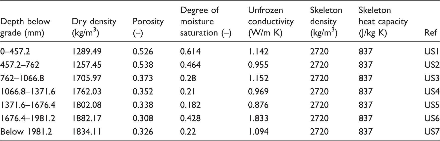
Material properties – undisturbed soil.

Depth below grade (mm)	Dry density (kg/m³)	Porosity (–)	Degree of moisture saturation (–)	Unfrozen conductivity (W/m K)	Skeleton density (kg/m³)	Skeleton heat capacity (J/kg K)	Ref
0–457.2	1289.49	0.526	0.614	1.142	2720	837	US1
457.2–762	1257.45	0.538	0.464	0.955	2720	837	US2
762–1066.8	1705.97	0.373	0.28	1.152	2720	837	US3
1066.8–1371.6	1762.03	0.352	0.21	0.969	2720	837	US4
1371.6–1676.4	1802.08	0.338	0.182	0.876	2720	837	US5
1676.4–1981.2	1882.17	0.308	0.428	1.833	2720	837	US6
Below 1981.2	1834.11	0.326	0.22	1.094	2720	837	US7

Table 2.

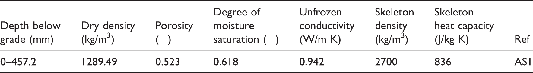
Material properties – agricultural silt.

Depth below grade (mm)	Dry density (kg/m³)	Porosity (−)	Degree of moisture saturation (−)	Unfrozen conductivity (W/m K)	Skeleton density (kg/m³)	Skeleton heat capacity (J/kg K)	Ref
0–457.2	1289.49	0.523	0.618	0.942	2700	836	AS1

Table 3.

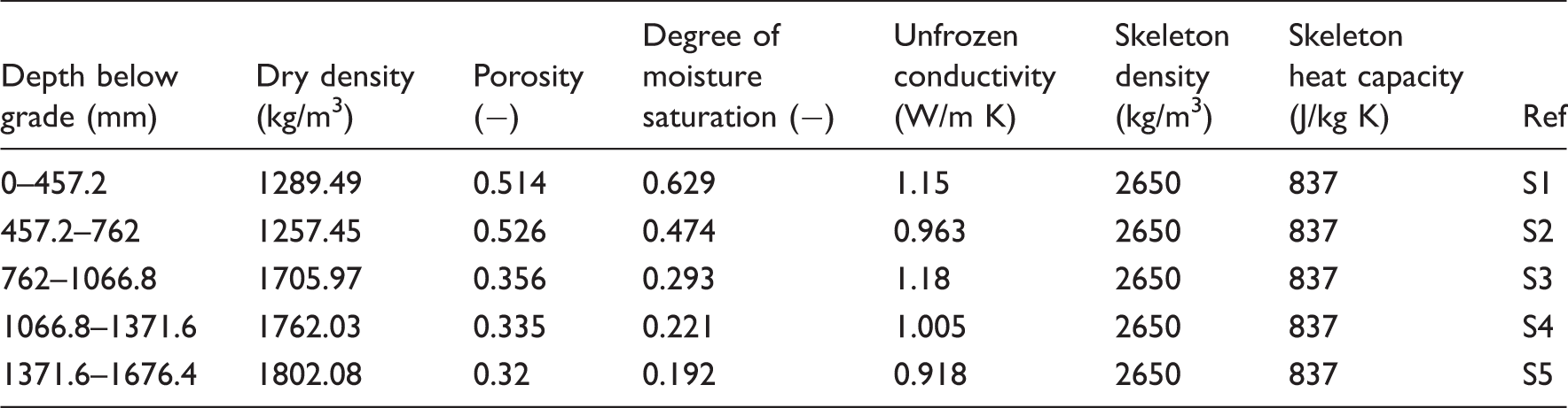
Material properties – uniform sand.

Depth below grade (mm)	Dry density (kg/m³)	Porosity (−)	Degree of moisture saturation (−)	Unfrozen conductivity (W/m K)	Skeleton density (kg/m³)	Skeleton heat capacity (J/kg K)	Ref
0–457.2	1289.49	0.514	0.629	1.15	2650	837	S1
457.2–762	1257.45	0.526	0.474	0.963	2650	837	S2
762–1066.8	1705.97	0.356	0.293	1.18	2650	837	S3
1066.8–1371.6	1762.03	0.335	0.221	1.005	2650	837	S4
1371.6–1676.4	1802.08	0.32	0.192	0.918	2650	837	S5

Table 4.

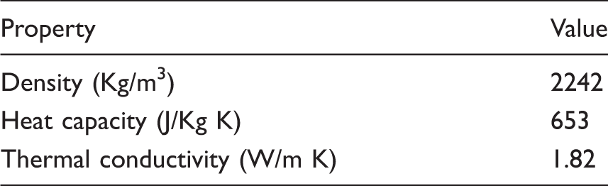
Material properties – concrete.

Property	Value
Density (Kg/m³)	2242
Heat capacity (J/Kg K)	653
Thermal conductivity (W/m K)	1.82

Table 5.

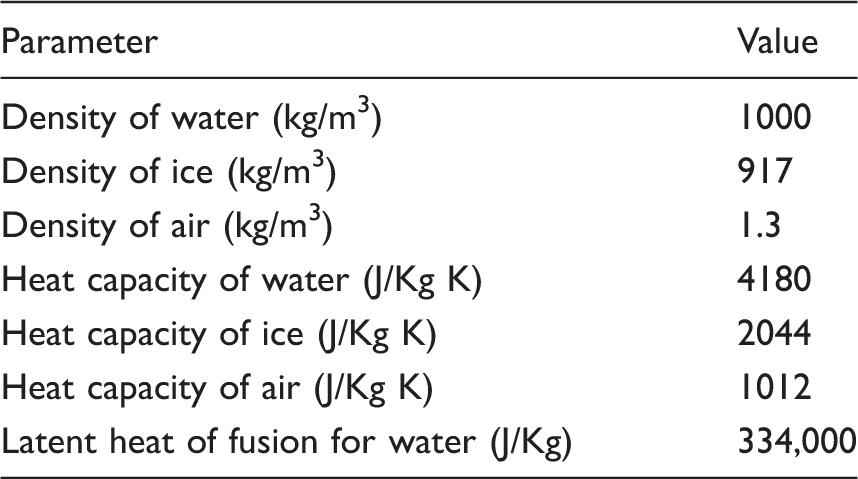
Physical parameters.

Parameter	Value
Density of water (kg/m³)	1000
Density of ice (kg/m³)	917
Density of air (kg/m³)	1.3
Heat capacity of water (J/Kg K)	4180
Heat capacity of ice (J/Kg K)	2044
Heat capacity of air (J/Kg K)	1012
Latent heat of fusion for water (J/Kg)	334,000

The Kersten number (K_e) is a function of the degree of saturation (S_r)

K_{e} ≅ 0.7 \log S_{r} + 1.0 clay content < 2 %

(9)

K_{e} ≅ \log S_{r} + 1.0 clay content > 2 %

(10)

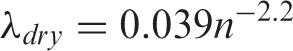
For completeness, the following semi-empirical power function is given for estimation of dry heat conductivity (λ_dry)

λ_{dry} = 0.039 n^{- 2.2}

(11)

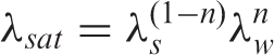
A geometric mean equation can be employed to define the saturated thermal conductivity (λ_sat)

λ_{sat} = λ_{s}^{(1 - n)} λ_{w}^{n}

(12)

where λ _w is the thermal conductivity of liquid phase and is taken as 0.58 W/mK. λ _s is the thermal conductivity of solid phase and can be determined from

λ_{s} = λ_{q}^{q} λ_{o}^{(1 - q)}

(13)

where, following Johansen,¹⁹ λ _q is the thermal conductivity of quartz and can be taken as 7.7 W/mK, λ _o is the thermal conductivity of other minerals and can be taken as 2.0 W/mK and q is the quartz content.

Finally, a modification to the unfrozen thermal conductivity is made, following the approach of Thomas et al.,¹³ to represent the impact of partial and total freezing of the soil water

λ_{T} = λ - (S_{i} . {nS}_{r}) \cdot (λ_{w} - λ_{i})

(14)

where λ _i is the thermal conductivity of the ice phase and is taken as 2.22 W/mK.

For the purpose of the subsequent numerical simulation, the distribution of material properties throughout the region considered is shown in Figure 5. In this manner, the variation of properties with depth, for each material type, can be represented.

Figure 5.

Material property representation.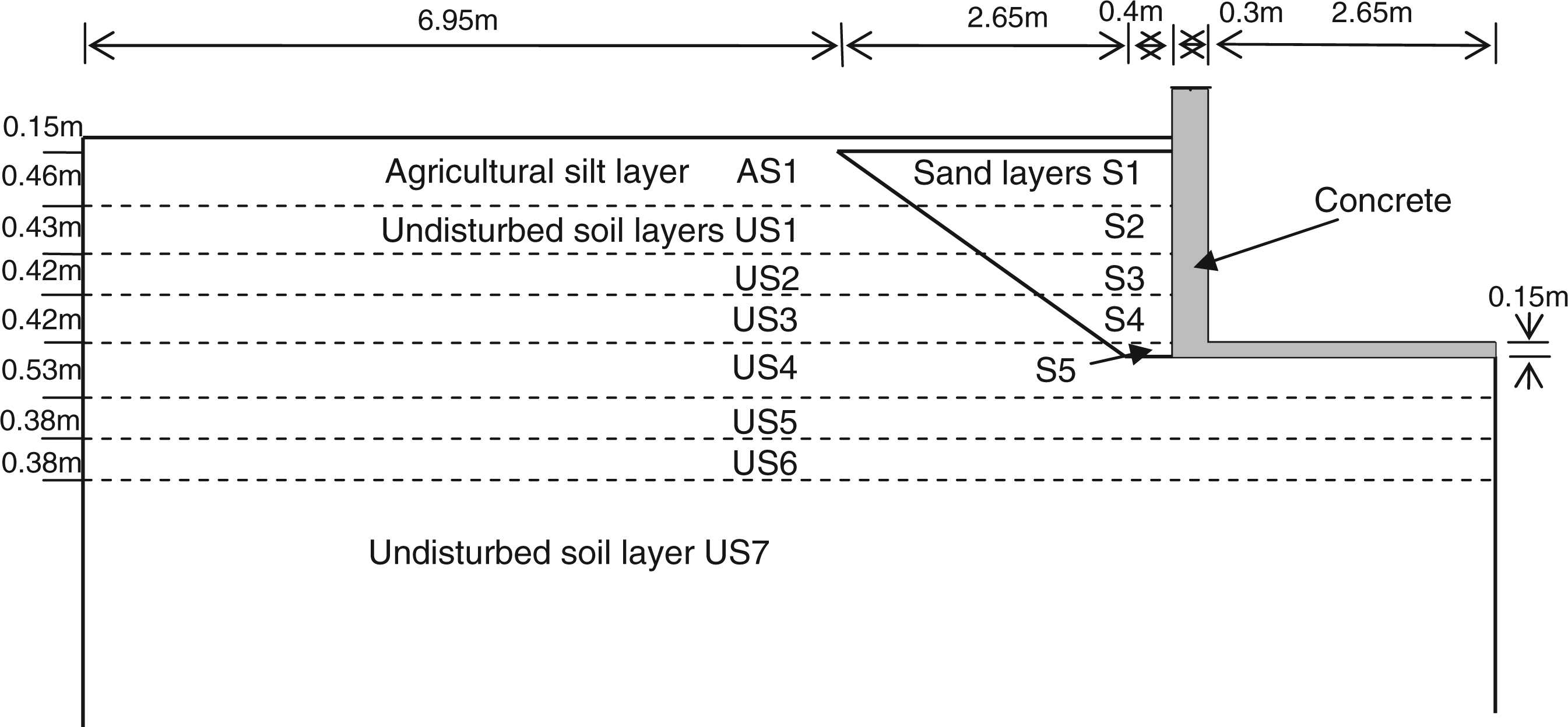

Numerical simulation

The domain shown in Figure 5 has been used as the basis for the formation of the finite element mesh shown in Figure 6. The mesh consists of 200 elements and 636 nodes. Quadrilateral, eight node elements are used for spatial discretisation.²⁰ The time-dependent nature of the solution is accommodated via an implicit mid-interval backward-difference algorithm.¹⁶ A fixed time-step size of 21,600 s was employed. Convergence of the spatial and temporal discretisation process has been considered previously¹¹ and the approach adopted here has been found to produce converged results. Spatial discretisation and the domain representation therefore facilitate inclusion of each individual material type and depth variation of soil properties within the following numerical simulations.

Figure 6.

Finite element mesh.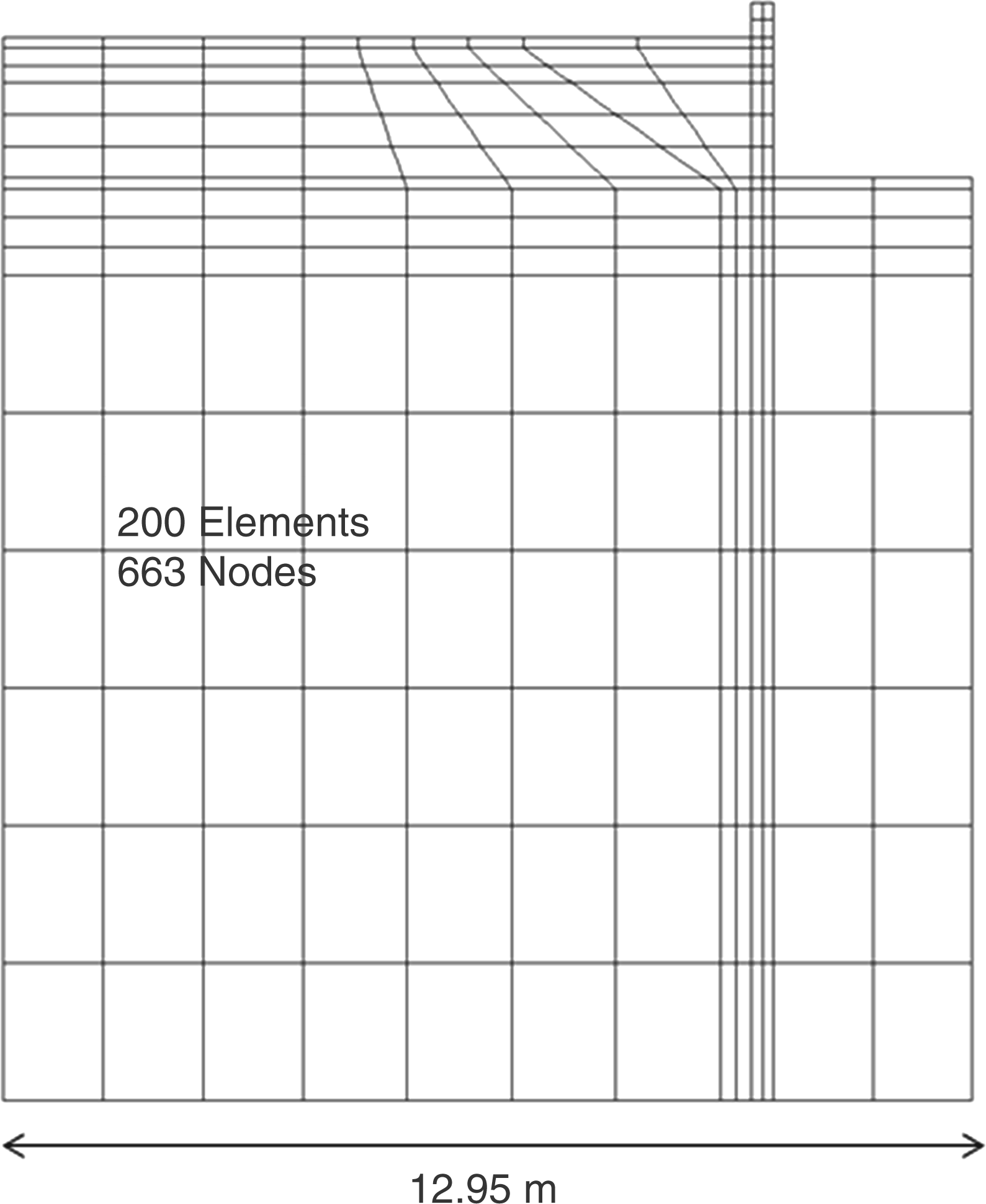

Three numerical simulations have been undertaken to explore the influence of soil-freezing processes and snow cover during the winter months. In terms of the processes considered, these simulations are presented in order of progressively increasing complexity allowing the impact of these various processes to be assessed. In summary, the simulations undertaken are

Simulation 1 – Provides a benchmark transient heat transfer simulation. The ‘corrected’ boundary conditions presented in Figure 4 are employed as time-varying Dirichlet boundary conditions prescribed on the external soil surface and on the internal surface of the building (wall and floor). Following Rees et al.,¹¹ the lower boundary is set at 8.8℃ and the remaining vertical boundaries are assigned a zero flux Neumann boundary condition. In this simulation, ice formation is included within the simulation via a non-linear heat capacity and thermal conductivity that are dependent on ice content (refer to equations (5) and (7), respectively). Latent heat of fusion is not considered so equation (4) is reduced to

Φ = H_{c} (T - T_{r})

(15)

Simulation 2 – Extends Simulation 1 to include latent heat of fusion effects due to phase change (refer to equation (4)).

Simulation 3 – Develops Simulation 2 to include representation of the insulating effect that a snow layer will create when present on the external soil surface.

Initial conditions in the system are obtained following the approach of Rees et al.¹¹ with a ‘pre-analysis’ simulation undertaken. This approach allows a realistic estimation of the non-homogenous temperature field at the start of the time period under consideration (i.e. 1 September 1990 to 30 April 1991). The approach consists of taking a uniform initial temperature across the whole domain, at a value equal to the average air temperature of the period 1 September 1989 to 31 August 1990 (namely 8.8℃), and then applying time-varying Dirichlet boundary conditions to the external soil surface and the internal surface of the building based on measured data for this time period (as presented in Figure 4). A Dirichlet boundary condition is applied to the lower boundary of the domain at a fixed temperature of 8.8℃ and a zero flux Neumann boundary condition is applied to the remaining surfaces. This analysis is repeated for three full cycles of the measured data (i.e. a pseudo 36-month analysis) and the results at 24 and 36 months compared to ensure that a stabilised set of initial conditions have been achieved. The analysis of the 243 day period from 1 September 1990 to 30 April 1991 is then made. It is recognised that, in some circumstances, rainfall may give rise to an advective flux at the surface, however, given the relatively low rainfall rate during this period (detailed above) this is excluded from consideration in this work.

It can be seen in Figure 4 that snow was present on the soil surface from 6 December 1990 to 10 March 1991 with the snow depth typically varying between 10 and 20 cm. The effect of this snow layer on the external soil surface will lead to a thermal buffering between the soil surface temperature and the measured air temperature. Therefore an attempt is made here to characterise the impact of this layer, via a one-dimensional analysis, to obtain an estimate of the soil surface temperature below the snow layer. The domain considered is a snow layer (with a set thickness of either 10 or 20 cm) plus a soil layer of 14.17 m. A time-varying Dirichlet boundary condition is applied to the snow surface based on measured data for the relevant time period and a Dirichlet boundary condition of 8.8℃ applied at the bottom of the domain. Suitable spatial and temporal convergence was obtained via trial and error. The thermal properties of snow depend on age, compaction and climatic conditions and typical values are readily available from the literature.²¹^–²³ Based on this information, a representative set of material parameters for snow, that correspond to the conditions present in the Minnesota case, have been selected, namely (a) snow density 300 kg/m³, (b) thermal conductivity 0.6 W/mK and (c) heat capacity 2090 J/kgK. Initial conditions from the results of Simulation 2 are taken for the soil and the snow temperature is set at an initial value of 0℃.

Results

Figures 7–10 present the transient temperature variations from of all three simulations for sensors W_L_09, W_L_08, W_L_06 and W_L_01, respectively (the positions of these sensors are indicated on Figure 2). Experimentally measured values at these locations are also shown and a RMSE value of the simulated results compared to the measured data for the whole period of the simulation given. While the individual simulation results are of interest, comparisons across the simulations are more informative of the systems behaviour. As such, a number of general observations about the results are made before a more detailed analysis of the different simulations is undertaken.

Figure 7.

Measured data and Simulations 1–3 for W_L_09.

Figure 8.

Measured data and Simulations 1–3 for W_L_08.

Figure 9.

Measured data and Simulations 1–3 for W_L_06.

Figure 10.

Measured data and Simulations 1–3 for W_L_01.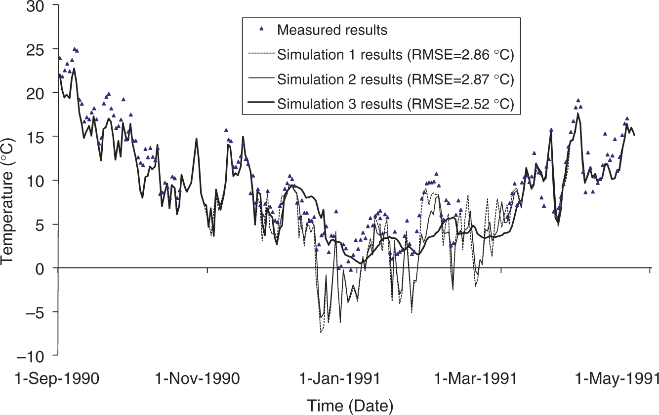

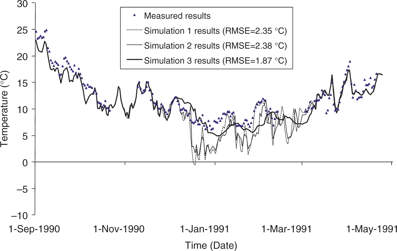
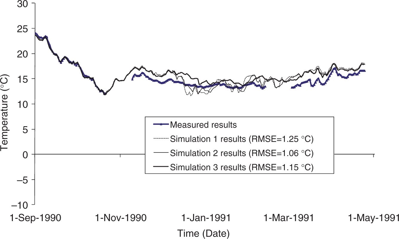
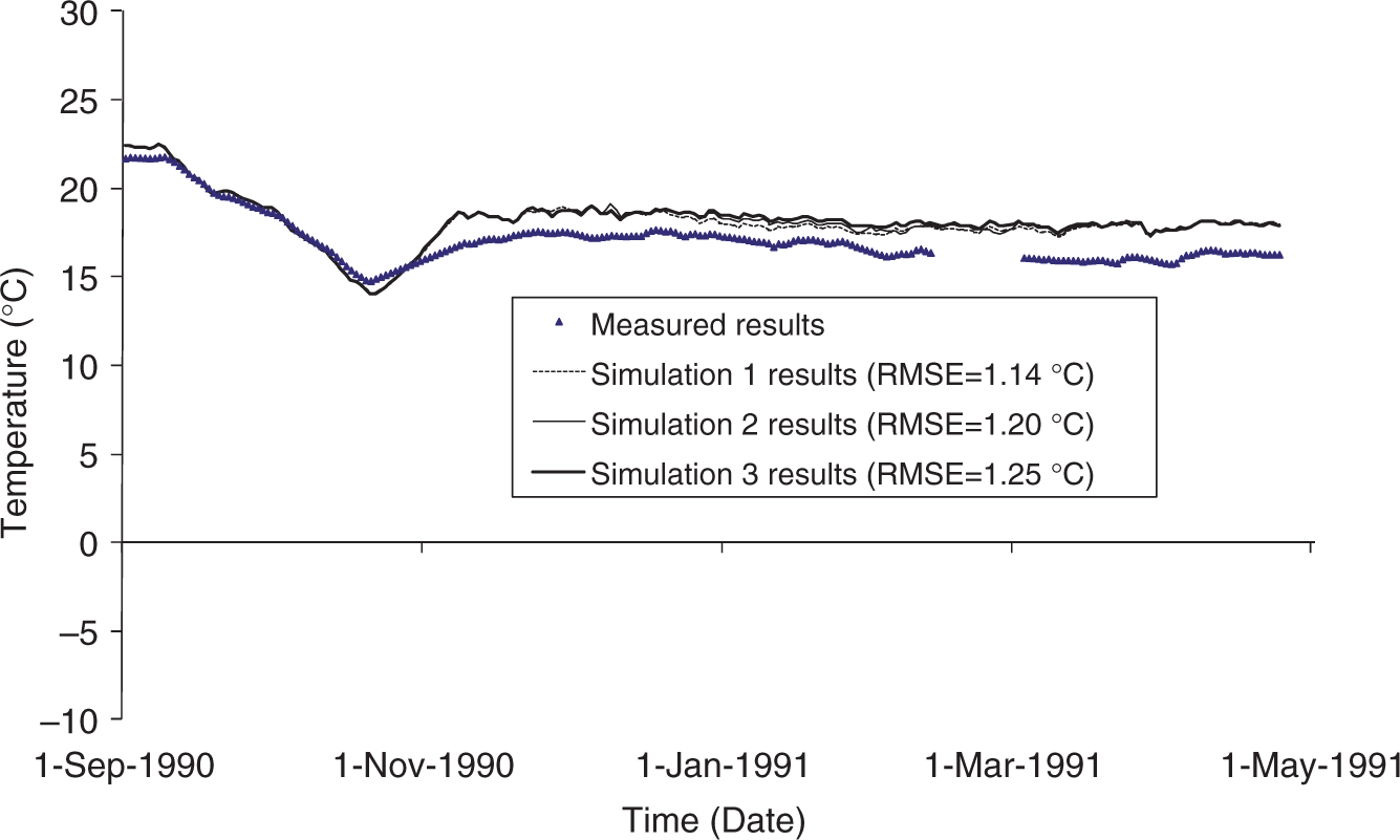
Comparison across the three simulations shows that, as would be expected, before the air temperature drops below 0℃, the results from each analysis are practically identical. During the period where air temperatures are below 0℃, there is a strong divergence between the results. Interestingly, after this period, in all regions the simulation results re-converge indicating that the impact of freezing, thawing and latent heat effects are relatively transient and do not appear to have a long-term impact on the thermal regime.

The simulation results show a very good correlation with the measured data before the air temperature drops below 0℃ for each of the four sensor locations. However, in the freezing period, only when latent heat effects are considered is the simulation able to reasonably capture the experimentally measured behaviour. An increasingly improving match between measured and simulated results is found with increasing depth, for example, the RMSE for Simulation 3 reduces from 2.52℃ at W_L_09 to 1.25℃ at W_L_01. The marked divergence between the measured and simulated data found after November 1990 at W_L_01 was also encountered by Rees et al.¹¹ who identified that this point was influenced by the 3D nature of the building geometry, which is not considered here.

To illustrate the spatial penetration of sub-zero temperature, an example contour plot is shown in Figure 11. This plot represents the temperature distribution predicted on 1st March 1991 for Simulation 1. The impact of the building structure on the system can be clearly seen with (a) the frozen zone of soil restricted to the region below bare soil and (b) the soil temperature below the building remaining appreciably above the average air temperature. These elevated temperatures are due to a combination of residual thermal energy from the inter-seasonal cycle and the continuous downward thermal flux from the building structure.

Figure 11.

Contour plot of temperature (℃) on 1 March 1991 (Simulation 1).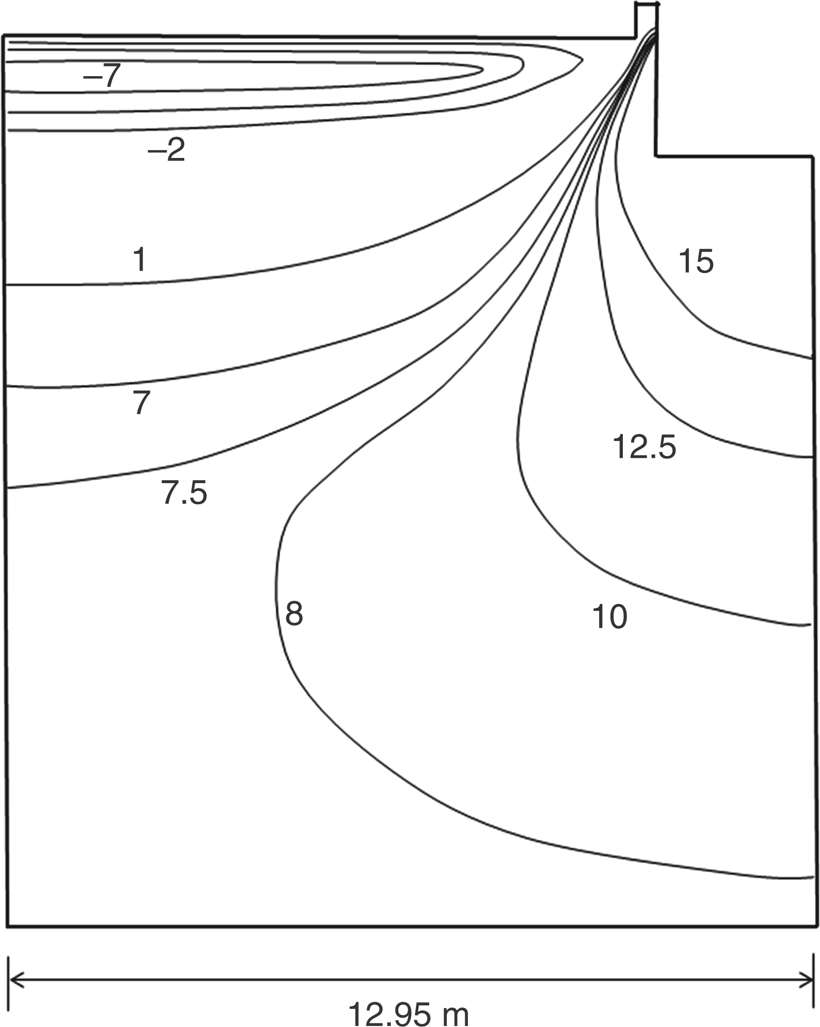

In Simulation 1, ice formation was included within the simulation via the non-linear heat capacity and thermal conductivity relations defined in equations (5) and (7), respectively. Latent heat of fusion is not considered in this simulation. Considering the depth of ice formation, it is clear that the heat transfer near the soil surface will be influenced to some extent. This is best illustrated via consideration of the thermal parameters in the soil layer nearest the ground surface (AS1). Equation (5) produced heat capacity variations between 2430 and 1684 kJ/m³K for the ice content variation generated in the simulation in this layer of agricultural silt. Similarly, thermal conductivity varied between 0.942 W/mK in the unfrozen soil and 1.472 W/mK when the ice content reached a maximum of 1.0.

The inclusion of latent heat effects is revealed by Simulation 2. The results are based on implementation of equation (4), with a latent heat of fusion for water of 334 kJ/kg resulting in a need for a removal of ∼99 MJ/m³ (in terms of total soil volume) of heat energy to achieve full freezing in the upper most layer (AS1). The impact of this process is exhibited in the results, for example in Figure 8, where the transient development of temperature in Simulation 2 can be seen to be delayed and damped in comparison to the results of Simulation 1 during times of freezing and thawing. This delay in temperature change is often termed the ‘zero curtain’ where the temperature at a specific point of soil being subjected to either freezing or thawing remains close to the segregation temperature, until complete freezing or complete thawing has occurred. The impact of these latent heat effects will be strongly controlled by the moisture content of the soil, which is considered in the model via the various layers defined in Tables 1 and 3 and equations (5) and (7) of the model. Subsequently, the decrease of moisture content with depth (see Table 3) will result in a decrease in the potential impacts of latent heat effects with depth. In comparison to Simulation 1, the RMSE values are relatively unchanged in the upper regions (W_L_09 and W_L_08) and show only small variations in the lower regions (W_L_06 and W_L_01) indicating that overall impact of including latent heat effects is relatively small. In terms of steady-state conditions, latent heat effects do not impact on the results, however, in terms of transient problems, they can result in an observable impact.

The presence of a layer of snow at the ground surface is considered in Simulation 3. Initial one-dimensional analyses have been undertaken to estimate the soil surface temperature below the snow layer. The results of these analyses, for the period 8 February 1991 to 10 March 1991, when the snow depth was approximately 10 cm are shown in Figure 12, with the measured surface air temperatures and the modelled soil surface temperatures presented. The insulating effect of the snow layer results in considerably lower variations in temperature at the soil surface (−2 to −8℃) than in the air (2 to −18℃), a similar variation was found in the period 6 December 1990 to 7 February 1991. These modified soil surface temperatures were then used in Simulation 3. The impact of the snow layer on the thermal response of the ground is clear in Figures 7–10 with considerably higher temperatures simulated, yielding a much closer correlation with the observed data. In terms of statistical measures, the RMSE values are significantly lower than those of Simulations 1 and 2 with a decrease in RMSE value, compared to Simulation 1, of 11.7% at W_L_09 and 20.3% at W_L_08. These differences are highlighted more clearly when only the period when snow cover is present (6 December 1990 to 10 March 1991) is considered, with decreases in RMSE values of 19% and 30.2% at W_L_09 and W_L_08 found, respectively.

Figure 12.

One-dimensional simulation of snow layer.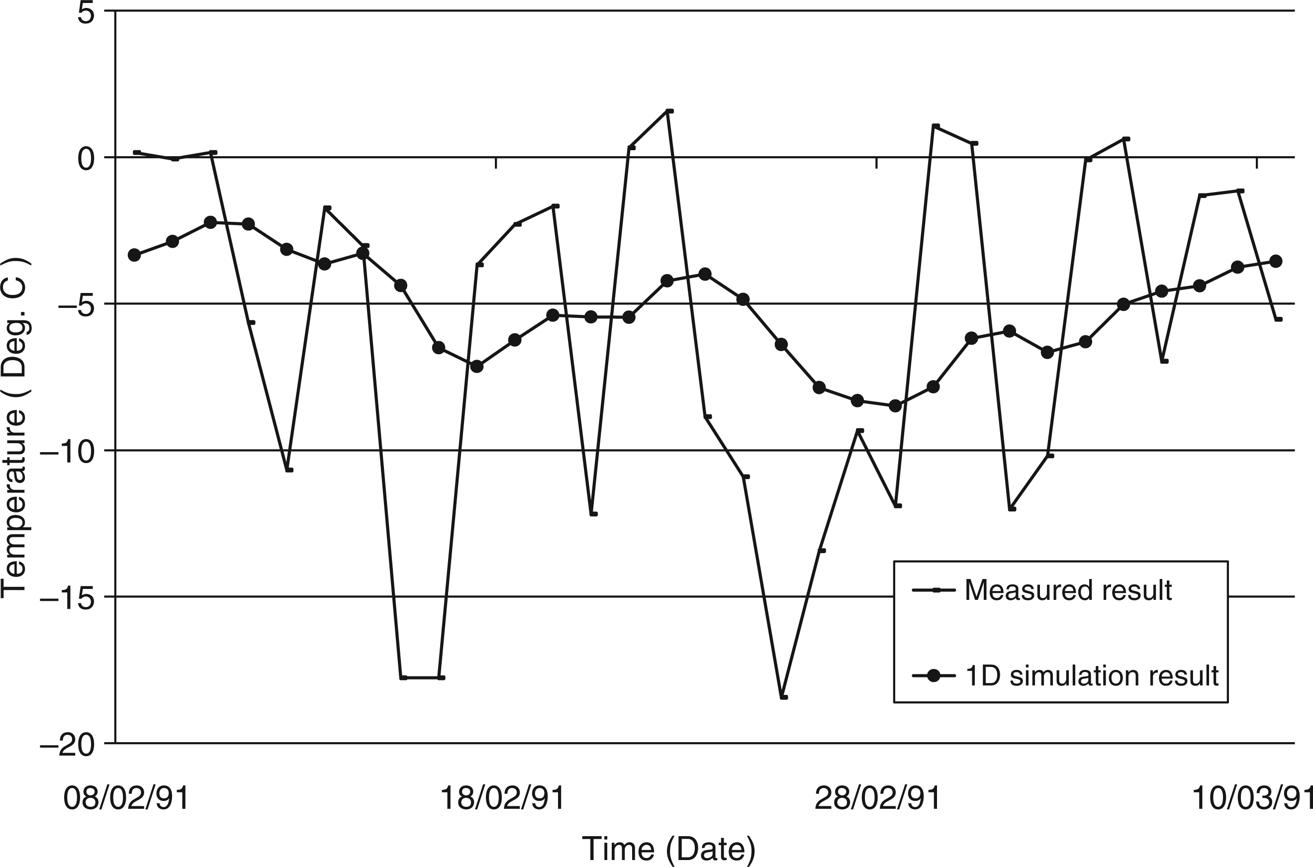

Conclusions

An approach for including the influence of soil freezing within the context of earth-contact ground heat transfer simulation has been presented. The model developed includes non-linear, ice content dependent, partial saturation, thermal conductivity and heat capacity. The formation of ice within the soil matrix as a function of temperature and time can be represented by the model. Latent heat effects due to phase change (between water and ice) and the impact of surface snow layers are also explored in the paper. The performance of the new model has been assessed via a series of numerical simulations that explore the influence of ground freezing on heat transfer patterns adjacent to a full-scale monitored building.

The results reveal the importance of correctly representing the impact of soil-freezing processes when considering earth-contact heat transfer. In particular, both the influence of ice content on thermal material parameters (namely conductivity and heat capacity) and latent heat of fusion are found to have an important impact on the thermal field. The importance of correctly representing soil surface boundary conditions has also been demonstrated with the necessity of capturing the impact of snow layers highlighted, via implementation of a simple modelling approach. Although the current work utilizes field data from the United States, the results would appear to suggest that simulation of near-surface ground heat transfer installations in the UK climate may benefit from similar treatment (particularly, given the relatively harsh winters of 2009 and 2010). However, further work is clearly required to make more definitive conclusions in this respect.

Footnotes

Funding

This research received no specific grant from any funding agency in the public, commercial or not-for-profit sectors.

Notation

References

Crosbie

Baker

. Energy-efficiency interventions in housing: learning from the inhabitants. Build Res Inform 2010; 38(1): 70–79.

Boardman

Darby

Killip

. 40% house, Oxford: Environmental Energy Change Institute, University of Oxford, 2005.

DEFRA – Department of Environment, Food and Rural Affairs. Climate change bill, http://www.defra.gov.uk (2009, accessed May 2011).

Zoras

. A review of building earth-contact heat transfer. Adv Build Energy Res 2009; 3(1): 289–314.

Brandl

. Energy foundations and other thermo-active ground structures. Geotechnique 2006; 56(2): 81–122.

Liu

Shi

Tang

. A numerical and field investigation of underground temperatures under urban heat island. Build Environ 2011; 46: 1205–1210.

Carder DR, Barker KJ, Hewitt MG, et al. Performance of an interseasonal heat transfer facility for collection, storage and re-use of solar heat from the road surface. TRL Published Project Report PPR302, 2008, Berks: TRL Ltd.

Krarti

. Analysis of heat and moisture transfer beneath freezer foundations—Part I. Transact ASME 2004; 126: 716–725.

Krarti

. Analysis of heat and moisture transfer beneath freezer foundations—Part II. Transact ASME 2004; 126: 726–731.

10.

Overduin

Kane

van Loon

WKP

. Measuring thermal conductivity in freezing and thawing soil using the soil temperature response to heating. Cold Regions Sci Technol 2006; 45: 8–22.

11.

Rees

Zhou

Thomas

. Multidimensional simulation of earth-contact heat transfer. Build Res Inform 2006; 34(6): 565–572.

12.

Shipp PH. Basement, crawlspace, and slab-on-grade thermal performance. In: Proceedings of ASHRAE/DOE conference on thermal performance of the exterior envelopes of buildings, Las Vegas, Nevada, 6–9 December 1982, 1983, pp.160–179.

13.

Thomas

Cleall

. Modelling of cryogenic processes in permafrost and seasonally frozen soils. Geotechnique 2009; 59(3): 173–184.

14.

Tice AR, Anderson DM and Banin A. The prediction of unfrozen water contents in frozen soils from liquid limit determinations. Alexandria, VA: CRREL US Army Corps of Engineers, 1976.

15.

De Vries

. In: Van Wisk

(ed.) Physics of plant environment, Amsterdam: North-Holland Publishing Company Ltd., 1966, pp. 211–235.

16.

Thomas

. Analysis of coupled heat, moisture and air transfer in a deformable unsaturated soil. Geotechnique 1995; 45: 677–689.

17.

Cleall

Seetharam

Thomas

. Inclusion of some aspects of chemical behaviour of unsaturated soil in thermo/hydro/chemical/mechanical models. I: model development. ASCE J Eng Mech 2007; 133(3): 338–347.

18.

Menne

Williams

Palecki

. On the reliability of the U.S. surface temperature record. J Geophys Res 2010; 115: p1–9, D11108–p1–9, D11108.

19.

Johansen O. Thermal conductivity of soils. PhD Thesis, University of Trondheim, Norway, 1975.

20.

Lewis

Morgan

Thomas

. The finite element method in heat transfer analysis, Oxford: John Wiley & Sons Ltd, 1996.

21.

Fukusako

. Thermophysical properties of ice, snow, and sea ice. Int J Thermophys 1988; 11(2): 353–372.

22.

Goodrich

. The influence of snow cover on the ground thermal regime. Can Geotechn J 1982; 19: 421–432.

23.

Woodside

. Calculation of the thermal conductivity of porous media. Can J Phys 1958; 36(7): 815–815.