Predictive performance of a wastewater source heat pump using artificial neural networks

Abstract

A pilot-scale wastewater source heat pump was operated for 30 days to recover heat from waste bathwater and to warm up fresh bathwater. The results indicated that the fresh water successfully warmed up to the designated 45℃, 50℃, and 55℃ with the coefficients of performance of 2.3–3.5. Artificial neural networks including back propagation, radial basis function, and nonlinear autoregressive model with exogenous input were used to simulate this process. The root-mean-square error and coefficient of variation of the simulated results, using the experimental data taken on the first 18, 21, 24, and 27 days, respectively, as a package of training data, showed that taking the data measured on more days as the training data improved simulation accuracy. The nonlinear autoregressive model with exogenous input needed at least 24 days’ training data to achieve acceptable simulation results, the back propagation needed 27 days, while the radial basis function did not achieve acceptable results. Predictions based on the nonlinear autoregressive model with exogenous input modeling showed that the performance of the wastewater source heat pump system could gradually be stabilized within 42 days.

Practical application: This study showed that the wastewater source heat pump can recover heat from waste bathwater to warm up fresh bathwater, and also demonstrated that the artificial neural network, especially nonlinear autoregressive model with exogenous input, is appropriate for predicting heat pump performance. Using this system can reduce building energy consumption, while using the artificial neural network model can help operate and maintain the wastewater source heat pump system.

Keywords

Wastewater source heat pump artificial neural network heat transfer capacity coefficients of performance

Introduction

A wastewater source heat pump (WWSHP) is considered as an environmentally friendly and energy-saving device,^1–4 and has been widely used for building heating and air conditioning in recent years.^5,6 Related studies found this method as feasible for recovering heat from urban sewage, dishwasher disposals, and waste bathwater with economic benefits.^7–9 Researchers have also noticed the challenges in collecting high-temperature wastewater, filtering large-sized particles, and cleaning fouling.^8,10 Bio-fouling, such as heterotrophic bacteria, microbial nutrients, and suspended substances,¹¹ can significantly reduce heat transfer efficiency.¹² Efforts have been made to experimentally examine the performance of WWSHP in various conditions. For example, Li et al.² applied WWSHP to generate heat for desalination, and found its coefficients of performance (COP) to be 3–11.

Numerical methods have also been applied to predict the performance of heat pump devices. In general, three modeling approaches have been used, i.e., the dynamic model, empirical model, and artificial neural network (ANN) model. To use dynamic models, a well-established dynamic theory about each part of the heat pump is required. However, the mechanism of fouling caused by waste water in a WWSHP is still not explicitly understood, which presents a technical hurdle in simulating the gradually deteriorating WWSHP performance. Likewise, fouling also invalidates the application of empirical models. As noted, there are six mechanisms involved in the waterside fouling, i.e., scaling, particulate, chemical reaction, corrosion, bio-fouling, and freezing.¹³ In a WWSHP, fouling on the surface of the heat exchanger is a complex issue that may involve multiple mechanisms due to the tangled driving factors. Besides, after cleaning, the fouling growth trend may be different from the previous cycle, which makes it difficult to develop an empirical model. The ANN has an excellent approximation and fast processing capacity^14,15 and can dynamically predict the performance of the WWSHP based on its current and past operating conditions. Therefore, the ANN model was selected to predict the performance of the WWSHP in this study.

Previous studies have employed the ANN technique to estimate potential outputs of refrigerant compressors,¹⁶ evaporative condensers,¹⁷ heat exchangers,¹⁸ and cooling coils,¹⁹ with successful outcomes. Commonly used ANN models are back propagation (BP),²⁰ radial basis function (RBF),²¹ the nonlinear autoregressive model with exogenous input (NARX),²² and the adaptive neuron fuzzy interface systems (ANFIS).²³ Esen et al.²⁴ used the BP model to simulate the performance of a horizontal ground-coupled heat pump and achieved excellent results in terms of 1% root-mean-squared error (RMSE), 99.999% of absolute fraction of variance (R²), and 28.62% of coefficient of variation (COV); Balcilar et al. applied the RBF model to determine the heat transfer coefficient and pressure drop of R134a inside of the vertical smooth tubes, and found that the predicted results were close to the experimentally measured results with ±5% deviations for all tested conditions;²⁵ Hayati et al.²⁶ worked on the ANFIS model to predict the heat transfer rate of a wire-on-tube type heat exchanger, and noted that the predicted values agreed with the actual values from the experiments with a mean relative error less than 2.55%. These studies demonstrated the feasibility of the ANN models for simulating heat pump performance, and also indicated that the application of the ANN models may depend on the type of heat source/sink and the structure of the tested devices. Selection of the ANN models, however, was addressed in previous studies, although it was generally believed that high accuracy, fast speed, and limited training data requirement were preferred.

Our previous study of the WWSHP using waste bathwater as a heat source has shown that its performance (heat transfer capacity, COP) was a function of a variety of factors, including inlet wastewater flowrate and temperature, inlet refrigerant flowrate and temperature, build-up of fouling, and so on. The involvement of multi-variations inspired us to consider using ANN to simulate the heat recovery process. Also, given the fact that factors such as build-up of fouling are often nonlinear,^11,27,28 ANN would be an effective tool in this case.²⁹ To our best knowledge, no such test has been carried out. Therefore, we hypothesize that the performance of the WWSHP system depends on its current and past performance. To test this hypothesis, a pilot-scale WWSHP system was built using waste bathwater as feedstock and was operated for 30 days. Measured results taken during a certain period of time were employed as training data so that the ANN model could predict the system performance on the following days. The objectives of this study are composed of: (i) examining the performance of the WWSHP using waste bathwater as a heat source; (ii) testing the feasibility of the ANN models in predicting the performance of the WWSHP system; three ANN models were selected, including BP, RBF, and NARX; and (iii) predicting performance of the WWSHP using the most appropriate ANN model.

Materials and methods

Experimental set-up

The pilot-scale WWSHP system was composed of three units: a wastewater collection and storage unit, a heat pump, and a fresh water heating unit (Figure 1). The wastewater tank (WWT) measured 0.9 m (L) × 0.7 m (W) × 1.2 m (H), inside which a wastewater pump (WP1) circulated wastewater into the heat pump. Heat was recovered and then was used to warm up fresh bathwater that was stored in a fresh water tank (FWT). After extraction of the heat, the wastewater was returned to the WWT. When temperature T₆ was lower than 26℃, the wastewater was drained off from the bottom of the WWT by the wastewater pump (WP2). Two-level sensors (LV801, OMEGA, Shanghai, China) were installed on the WWT, and were used to maintain the wastewater in the WWT at an appropriate level by regulating the solenoid valves (SV). Wastewater temperature inside of the WWT was measured along its centerline, 1080 mm (T₄), 750 mm (T₅), and 50 mm (T₆) above the bottom using platinum-resistance thermometers (range: −50 to 500℃; accuracy: ±0.1℃). Flowrates of the two WPs were measured using flow meters (range: 0.1–11.8 m³/h; accuracy: ±1.5%; Omega, FTB8010B-PT, Stamford, CT, USA). The fresh water at the inlet of the FWT had a temperature of about 26℃ (T₃), and was warmed up in the FWT. When the temperature (T₂) reached a high limit (T_HL), the hot fresh water was drained off from the top of the FWT, and the cool fresh water was compensated from the bottom of the FWT. 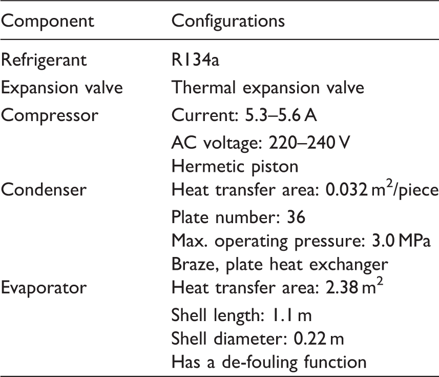The selected shell-and-tube evaporator had a de-fouling function that was described in detail in a previous study.¹² Electric consumption was recorded continuously using a current meter (range: 0–20 A, accuracy: ±0.5%, YOKOGAWA-CW120, Chelmsford Essex, England) and a voltage meter (range: 0–400, accuracy: ±0.5%, YOKOGAWA-CW120, Chelmsford Essex, England). Data were recorded every 30 s using a data logger (Model: SWP-NSP-M, Changhui, Hongkong SAR). Specifications of the WWSHP are given in Table 1.

Figure 1.

Schematic design of the experimental set-up: FWT – fresh water tank; PC – plate condenser; EX – expansion valve; CO – compressors; EV – evaporator; WP1 – wastewater pump 1; WP2 – wastewater pump 2; WWT – wastewater tank; SV – solenoid valve; LS – level sensor; FM – flowrate meter; T – temperature sensor; P – pressure sensor.

Table 1.

Wastewater source heat pump specifications.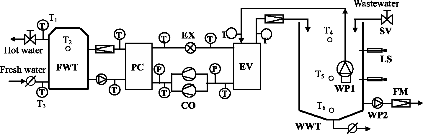

Component	Configurations
Refrigerant	R134a
Expansion valve	Thermal expansion valve
Compressor	Current: 5.3–5.6 A
	AC voltage: 220–240 V
	Hermetic piston
Condenser	Heat transfer area: 0.032 m²/piece
	Plate number: 36
	Max. operating pressure: 3.0 MPa
	Braze, plate heat exchanger
Evaporator	Heat transfer area: 2.38 m²
	Shell length: 1.1 m
	Shell diameter: 0.22 m
	Has a de-fouling function

Experimental procedure and performance evaluation

The system was designed to provide warm bathwater with the T_HL designated to be 45℃, 50℃, or 55℃. For each condition, five heating processes were conducted and each process took about 30 min. One heating process refers to the procedure of warming the fresh bathwater in the FWT to the desired temperature. The system was operated for 30 days.

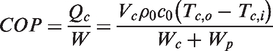
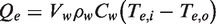
Six operating parameters were monitored, including operating time, inlet wastewater temperature, inlet freshwater temperature, outlet freshwater temperature, and flowrate of WP1 and WP2. Then, the system COP and the evaporator heat transfer capacity were calculated using equations (1) and (2).

COP = \frac{Q_{c}}{W} = \frac{V_{c} ρ_{0} c_{0} (T_{c, o} - T_{c, i})}{W_{c} + W_{p}}

(1)

Q_{e} = V_{w} ρ_{w} C_{w} (T_{e, i} - T_{e, o})

(2)

where Q_c and Q_e: heat transfer capacity of the condenser and the evaporator, respectively; W: total system power consumption, include W_c (two compressors) and W_p (one freshwater pump and two WPs); V_c: condenser wastewater flowrate; V_w: evaporator wastewater flowrate; ρ₀ and c₀: density and specific heat of freshwater, respectively; ρ_w and c_w: density and specific heat of wastewater, respectively; T_c,i and T_c,o: freshwater temperature at the inlet and outlet of the condenser; T_e,i and T_e,o: wastewater temperature at the inlet and outlet of the evaporator.

The daily averaged results of the COP, heat transfer capacity of evaporator, and refrigerant evaporating temperature were used for the ANN simulation and are reported in this paper.

Artificial neural network analysis

Three ANN models, including the BP, RBF, and NARX methods, were examined in this study with the purpose of testing their feasibilities in predicting the performance of the WWSHP system. Descriptions about these three networks can be found in many previous studies;^21,29,30 therefore, they were only briefly introduced here. As a multi-layer feed-forward neural network, the BP model has an input layer, an output layer, and one or more hidden layers. A schematic form of an artificial neuron model is shown in Figure 2(a). In multi-layer feed-forward networks, neurons are arranged in layers and there is a connection among the neurons in neighboring layers. However, the second model RBF (Figure 2(b)) is embedded in a two-layer neural network, where each hidden layer implements a radial activated function. The inputs of an RBF network are nonlinear while its outputs are linear and implement a weight sum of hidden layer outputs. The third model NARX is a recurrent dynamic network, with feedback connections enclosing several layers of the network. This model relates the current value of a time series which one would like to explain or predict to both past values of the same series and current and past values of the driving (exogenous) series. A diagram of the resulting network of NARX is shown in Figure 2(c).

Figure 2.

Network models. (a) Back propagation artificial neuron (BP); (b) Radial basis function (RBF); and (c) nonlinear autoregressive model with exogenous input (NARX).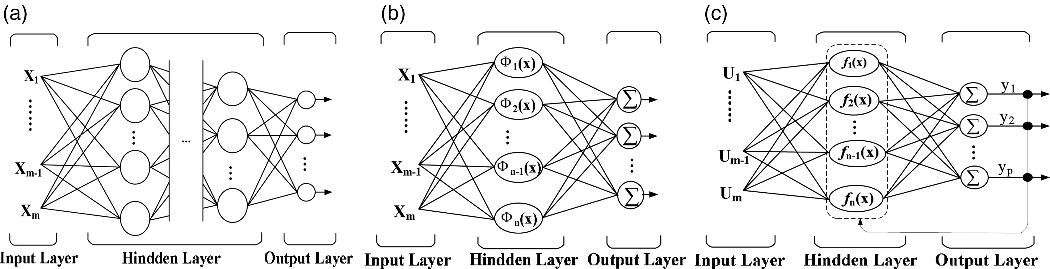

Experimental data were used as the training data to train these three models, respectively. In order to find out which ANN model could achieve an acceptable accuracy based on less training data, experimental data taken on different continuous days were used as the training data for each ANN model. In each training process, all the training data were divided into three contiguous sets. In all, 70% of the data was used as the first set for the training, 15% of the data was used as the second set for validation and the remaining 15% was used as the third set for testing. This training model was used to predict the system performance (evaporating temperature, heat transfer capacity, COP) for the following three days. The predicted results were then compared to the measured data of those three days. To compare the feasibility of the three models in this report, only the comparison results (between the predicted data and the experimental data taken on the following three days) based on the training experimental data taken on first continuous 18 days (means from the 1st day to the 18th day), first 21 days, first 24 days, and first 27 days were presented selectively, which represents the comparison results distinctly.

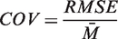
For comparison purposes, the daily system performance under the three working conditions (T_HL = 45℃, 50℃, and 55℃) was combined together; thus, for each output operating parameter, nine data (three conditions/day × three days) were obtained. Paired Student’s t tests were conducted to compare the predicted data and the measured data. The RMSE and COV of the predicted data were calculated using the following two equations³⁰

RMSE = \sqrt{\frac{\sum_{i = 1}^{n} (P_{i} - M_{i}) 2}{n}}

(3)

COV = \frac{RMSE}{\bar{M}}

(4)

where P_i: predicted value of data i; M_i: measured value of data i; n: number of data, equal to 9;

\bar{M}

: mean value of measured data.

If the COV of all three operating parameters (evaporating temperature, heat transfer capacity, and COP) was lower than 0.02, the simulated results were considered acceptable; otherwise, the simulation requires improvement, and more training data (measured on more days) should be applied.

Uncertainty analysis

Parameter uncertainty was estimated according to Holman’s method³¹ as shown in equation (5)

W_{r} = [(\frac{\partial R}{\partial x_{1}} w_{1}) 2 + (\frac{\partial R}{\partial x_{2}} w_{2}) 2 + \dots + (\frac{\partial R}{\partial x_{n}} w_{n}) 2] 0.5

(5)

where W_r: total uncertainty; R: function of interested, R = f(x₁, x₂ , … , x_n); x_i: independent variable; w_i: uncertainty of each independent variable, which was obtained based on sensor resolution and accuracy.

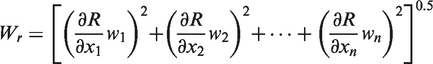
The maximum uncertainty of T₁, T₃, T₄, WP1 flowrate, WP2 flowrate, evaporating temperature, evaporator heat transfer capacity, and system COP was 0.3%, 0.4%, 0.4%, 2%, 2%, 1.2%, 4.2%, and 5.6%, respectively.

Results and discussion

System performance

Warm freshwater was produced at a desired temperature with minor fluctuations in all three working conditions during the 30-day operation (Figure 3(a)), showing the reliability of the WWSHP system. The outlet freshwater temperature, T₁, was 0–1.5℃ higher than the designated T_HL, mainly due to the vertical temperature gradient in the FWT with a slightly higher temperature in the upper layer compared to the lower layer. Note that the stable function of the system was achieved with the supply of ∼29℃ wastewater and ∼26.7℃ freshwater (Table 2). The wastewater circulating rate in the evaporator was 4–5 times higher than the wastewater drain off rate.

Figure 3.

System performance at three operating conditions. (a) Temperature of warm fresh water (T₁), (b) heat transfer capacity, and (c) COP. Hollow circle: T_HL = 55℃; grey diamond: T_HL = 50℃, black triangle: T_HL = 45℃.

Table 2.

System performance at three operating conditions.

T_HL ℃	T₃ ℃	T₄ ℃	Evap. temp., ℃	WP1 flowrate L/s	WP2 flowrate L/s
45	26.63 ± 0.37	28.90 ± 0.39	9.59 ± 0.62	1.28 ± 0.04	0.28 ± 0.05
50	26.70 ± 0.51	29.07 ± 0.71	10.12 ± 0.71	1.29 ± 0.04	0.30 ± 0.06
55	26.72 ± 0.40	29.05 ± 0.46	10.83 ± 0.98	1.29 ± 0.04	0.28 ± 0.05

WP: wastewater pump.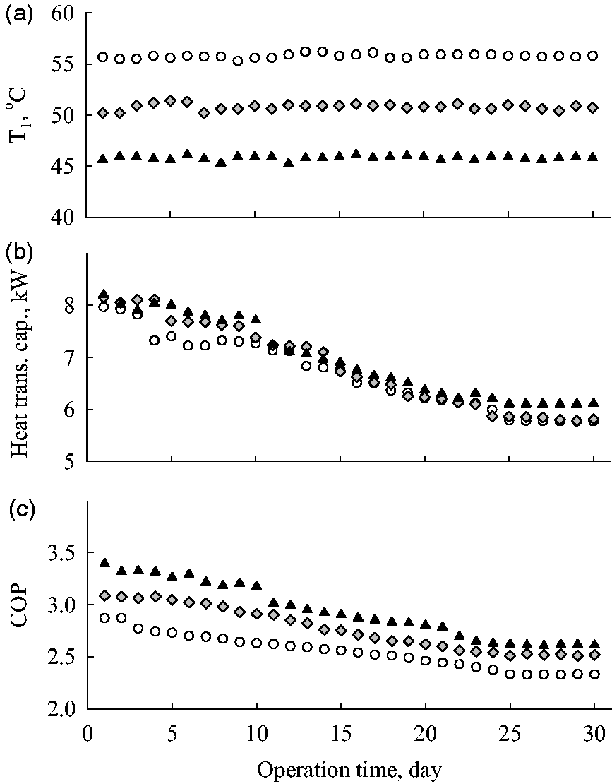

The heat transfer capacity of evaporator gradually dropped from about 8 kW to 6 kW in all three tests. The initial COP was 3.5 at T_HL of 45℃, but decreased during the test and became relatively stable on days 25–30 at 2.6. Similar trends were observed for the T_HL of 50℃ and 55℃. The lowest COP was 2.3. The primary reason for these decreases was the build-up of fouling on the surface of the heat exchangers which reduced the performance of the evaporator. A higher COP and a lower evaporating temperature were observed when the T_HL was set to 45℃, then followed by 50℃ and 55℃. As shown in Figure 3(b) and (c), the trends were not linear, which favors application of the ANN models.

Feasibility of ANNs

Statistical analysis showed that the predicted results were not significantly different from the measured data with p < 0.05 for all cases. For all three models and their three output parameters, the results showed that the differences between the predicted data and the measured data were generally large using 18-day training data; the differences were reduced if more training data (measured on more days) were employed, indicating that using ANN depends on the amount of available training data (Figure 4) while users would like to employ ANN models that require a small amount of training data but have acceptable predicted results.

Figure 4.

Comparison of ANN simulation results based on training data of: (a) 18 days, (b) 21 days, (c) 24 days, and (d) 27 days.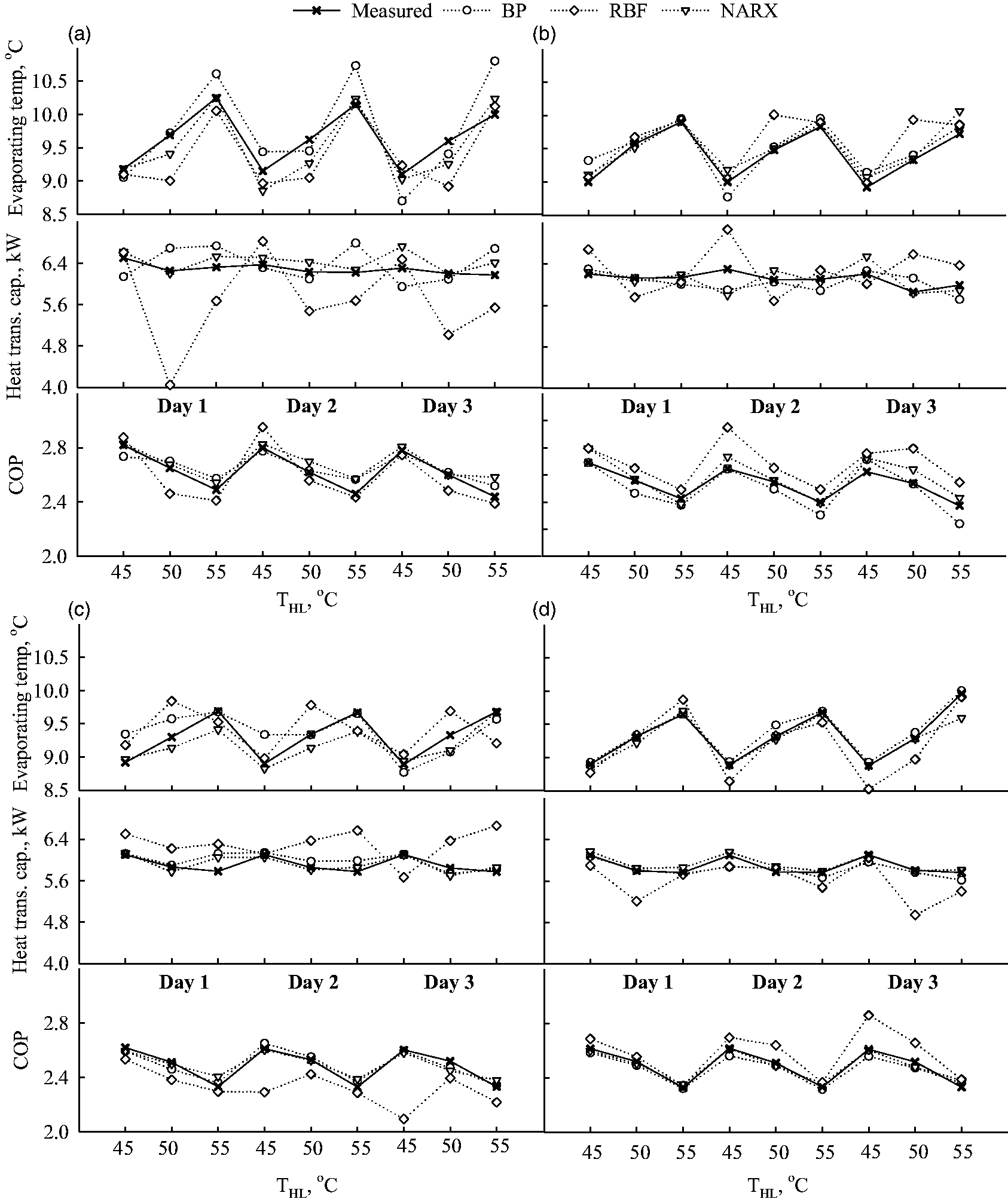

With regard to the evaporating temperature, the BP- and NARX-predicted results increased with the designated T_HL, while mixed trends were observed for the RBF-predicted results. The difference between the predicted data and the measured data was dramatically reduced when compared to the results using 18-day and 21-day training data (Figure 4). RMSE and COV were significantly decreased, and the COV of BP and NARX predicted results was lower than 0.02 using the 21-day training data (Table 3). However, using 24-day training data, did not improve the prediction accuracy, and only the NARX method achieved acceptable results (COV < 0.02). With 27-day training data, both BP- and NARX-predicted results were acceptable, and the COV of RBF-predicted results was very close to 0.02.

Table 3.

RMSE and COV results.

Days	Model	Evaporating temp.		Heat transfer capacity		COP
Days	Model	RMSE	COV	RMSE	COV	RMSE	COV
18	BP	0.400	0.042	0.371	0.059	0.063	0.024
	RBF	0.391	0.041	0.955	0.152	0.100	0.038
	NARX	0.232	0.024	0.196	0.031	0.070	0.027
	BP	0.164	0.017^a	0.210	0.034	0.074	0.0298
21	RBF	0.278	0.029	0.455	0.074	0.166	0.066
24	NARX	0.146	0.016^a	0.218	0.036	0.071	0.028
	BP	0.244	0.026	0.146	0.025	0.034	0.014^a
	RBF	0.340	0.037	0.551	0.093	0.218	0.088
	NARX	0.179	0.019^a	0.115	0.019^a	0.044	0.018^a
27	BP	0.067	0.007^a	0.112	0.019^a	0.035	0.014^a
	RBF	0.205	0.022	0.395	0.067	0.114	0.046
	NARX	0.131	0.014^a	0.060	0.010^a	0.027	0.011^a

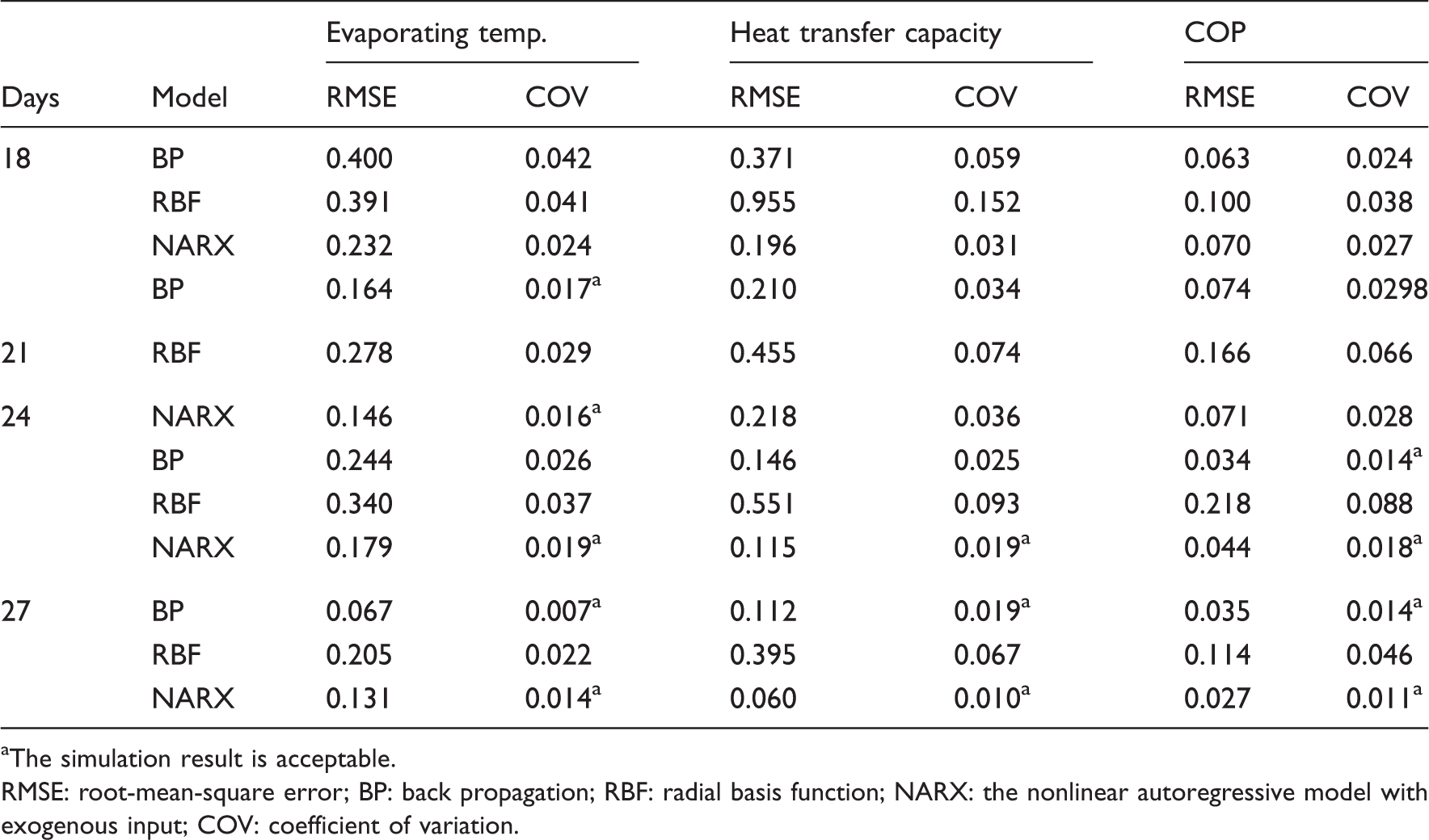
The simulation result is acceptable.

RMSE: root-mean-square error; BP: back propagation; RBF: radial basis function; NARX: the nonlinear autoregressive model with exogenous input; COV: coefficient of variation.

With regard to the heat transfer capacity, the RBF-predicted results were very active using 18-day training data, although the trend of measured data was relatively flat (Figure 4(a)); the simulation quality was improved by using more training data taken on more days. However, the COV (0.067) of the RBF method was still much higher than 0.02 when the 27-day training data were used (Table 3). The BP and NARX results were much closer to the measured data compared to the RBF-predicted results. The COV of BP and NARX became lower than 0.02 if 27-day and 24-day training data were used, respectively.

With regard to the system COP, it decreased with increased T_HL, and the predicted data were all quite close to the measured data, although RBF had a few points that were significantly shifted (Figure 4). The RBF-predicted COP using 24-day training data was lower than the measured data for all nine points, but was higher using 21-day and 27-day training data, indicating that this method was not reliable. Both BP and NARX methods achieved acceptable COV results using 24-day and 27-day training data.

Combining the above observations together, the NARX method displayed the highest prediction accuracy while RBF showed the lowest. The COV of the NARX method-predicted results was lower than 0.02 using 24-day training data and further decreased when using 27-day training data for all three system outputs (Table 3). The COV of the BP-predicted COP result was lower than 0.02 using 24-day training data, but not for evaporating temperature or heat transfer capacity; they achieved this goal when 27-day training data were used, indicating more training data are needed to obtain acceptable predicted results (Table 3). However, the COV of the RBF-predicted results was still higher than 0.02 for all three system outputs using 27-day training data, although their COV values decreased when compared to the results when less training data were applied. A group of training data taken on more than 27 days is needed for the RBF method.

Stability of WWSHP

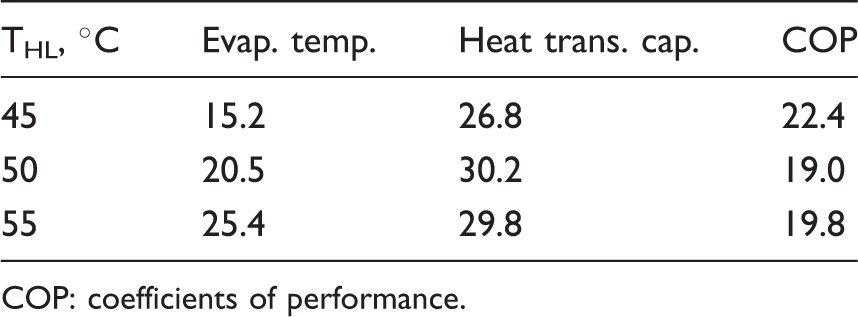
The performance of the WWSHP on following days (from the 31st to 42nd day) was further predicted using the NARX model. The performance on continuous three days (for instance, the 31st to 33rd day, or the 34th to 36th day) was predicted as a group and the experimental/predicted data of previous 24 days (from the 7th to 30th day for the prediction on the 31st to33rd day, from the 10th to 33rd day for the prediction on the 34th to 36th day) were used as the training data. The results are shown in Figure 5; it indicates that the evaporating temperature was slightly decreased and stabilized at 8.7 and 9.0℃ for the T_HL of 45℃ and 50℃, respectively, while the evaporating temperature was relatively constant (9.7℃) at the T_HL of 55℃. Similar phenomena were observed for the heat transfer capacity and the COP. Note that the heat transfer capacity decreased 3–5% before being stabilized for the T_HL of 45℃ and 50℃. Given the reliability of the NARX in predicting the WWSHP performance (Table 3), it is reasonable to consider the predicted results as the performance in the actual tests without extra artificial fouling cleaning. Compared to the initial system performance, the values of the three operating parameters dropped by 15–30%, as shown in Table 4, indicating a necessity for system cleaning and refreshing.

Figure 5.

Prediction of WWSHP performance on days 31–42: (a) evaporating temperature, (b) Heat transfer capacity, and (c) COP.

Table 4.

Percentage decreases of three output parameters.

T_HL, ℃	Evap. temp.	Heat trans. cap.	COP
45	15.2	26.8	22.4
50	20.5	30.2	19.0
55	25.4	29.8	19.8

COP: coefficients of performance.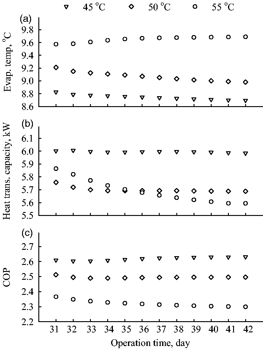

Conclusions

A WWSHP with a de-fouling function was operated for 30 days. The system successfully recovered heat from waste bathwater and warmed up fresh bathwater to the desired 45℃, 50℃, and 55℃ with a COP of 2.3–3.5. Three ANN models, including BP, NARX, and RBF, were used to predict the performance of the WWSHP in terms of evaporating temperature, heat transfer capacity, and COP. Statistical analysis results showed that the NARX model can accurately predict the system performance using at least 24-day training data, the BP model can achieve this goal by using at least 27-day training data, while the RBF model was not able to accurately predict system performance. Thus, the NARX model was selected to continue predicting the WWSHP performance. The results indicated that the performance of the WWSHP system would be stabilized within 42 days. The decrease of the system performance suggested that fouling cleaning is necessary for the WWSHPs.

Footnotes

Funding

The authors wish to acknowledge the financial support from the 12th Five-Year Science and Technology Support Program (No. 2012BAJ06B02) and (No. 2013BAJ12B03), and the University of Illinois at Urbana-Champaign.

Conflict of interest

None declared.

References

Hawley

Fenner

. The potential for thermal energy recovery from wastewater treatment works in southern England. J Water Clim Change 2012; 3: 287–299.

Russell

Sharifi

. Techno-economic feasibility of absorption heat pumps using wastewater as the heating source for desalination. Desalination 2011; 281: 118–127.

Baek

Shin

Yoon

. A study on the design and analysis of a heat pump heating system using wastewater as a heat source. Sol Energy 2005; 78: 427–440.

Funamizu

Iida

Sakakura

. Reuse of heat energy in wastewater: implementation examples in Japan. Water Sci Technol 2001; 43: 277–285.

Zhao

Zhang

. Study of the performance of an urban original source heat pump system. Energy Convers Manag 2010; 51: 765–770.

Vaiopoulou

Melidis

Aivasidis

. Process control, energy recovery and cost savings in acetic acid wastewater treatment. J Hazard Mater 2011; 186: 1141–1146.

Paepe

Theuns

Lenaers

. Heat recovery system for dishwashers. Appl Therm Eng 2003; 23: 743–756.

Liu

Jiang

. Application of an exhaust heat recovery system for domestic hot water. Energy 2010; 35: 1476–1481.

Shen

Jiang

Yao

. A field study of a wastewater source heat pump for domestic hot water heating. Build Serv Eng Res Technol 2012; 34: 433–448.

10.

Song Y, YaoY, Ma Z, et al. Study on performance of heat pump using in sewage treatment and fouling impact on system. In: ICEBO (Proceedings of the Sixth International Conference for Enhanced Building Operations), Shenzhen, 2006.

11.

Tian

Chen

Yang

. Effect of calcium ions on the evolution of biofouling by Bacillus subtilis in plate heat exchangers simulating the heat pump system used with treated sewage in the 2008 Olympic Village. Colloids Surf B 2012; 94: 309–316.

12.

Shen

Jiang

Yao

. Experimental performance evaluation of a novel dry-expansion evaporator with defouling function in a wastewater source heat pump. Appl Energy 2012; 95: 202–209.

13.

Webb

. Principles of enhanced heat transfer, New York: John Wiley and Sons, 1994.

14.

Bechtler

Browne

Bansal

. New approach to dynamic modelling of vapour-compression liquid chillers: artificial neural networks. Appl Therm Eng 2001; 21: 941–953.

15.

Mohanraj

Jayaraj

Muraleedharan

. Applications of artificial neural networks for refrigeration, air-conditioning and heat pump systems-A review. Renew Sustain Energy Rev 2012; 16: 1340–1358.

16.

Yang

Zhao

Zhang

. Loss-efficiency model of single and variable-speed compressors using neural networks. Int J Refrigeration-Revue 2009; 32: 1423–1432.

17.

Ertunc

Hosoz

. Artificial neural network analysis of a refrigeration system with an evaporative condenser. Appl Therm Eng 2006; 26: 627–635.

18.

Pacheco-Vega

Sen

Yang

. Neural network analysis of fin-tube refrigerating heat exchanger with limited experimental data. Int J Heat Mass Transfer 2001; 44: 763–770.

19.

Yigit

Ertunc

. Prediction of the air temperature and humidity at the outlet of a cooling coil using neural networks. Int Commun Heat Mass Transfer 2006; 33: 898–907.

20.

Mohanraj

Jayaraj

Muraleedharan

. Performance prediction of a direct expansion solar assisted heat pump using artificial neural networks. Appl Energy 2009; 86: 1442–1449.

21.

Kalogirou

. Artificial intelligence for the modeling and control of combustion processes: a review. Prog Energy Combust Sci 2003; 29: 515–566.

22.

Mellit

Kalogirou

. Artificial intelligence techniques for photovoltaic applications: a review. Prog Energy Combust Sci 2008; 34: 574–632.

23.

Jang

. ANFIS – adaptive-network-based fuzzy inference system. IEEE Trans Syst Man Cybern 1993; 23: 665–685.

24.

Esen

Inalli

Sengur

. Performance prediction of a ground-coupled heat pump system using artificial neural networks. Expert Syst Appl 2008; 35: 1940–1948.

25.

Balcilar

Dalkilic

Wongwises

. Artificial neural network techniques for the determination of condensation heat transfer characteristics during downward annular flow of R134a inside a vertical smooth tube. Int Commun Heat Mass Transfer 2011; 38: 75–84.

26.

Hayati

Rezaei

Seifi

. Prediction of the heat transfer rate of a single layer wire-on-tube type heat exchanger using ANFIS. Int J Refrigeration-Revue 2009; 32: 1914–1917.

27.

Daniels

Selby

. Biofouling control options for cooling systems. Power 2007; 151: 58–65.

28.

Flemming

Schaule

. Microbial deterioration of materials – biofilm and biofouling – biofouling. Mater Corros 1994; 45: 29–39.

29.

Esen

Inalli

. ANN and ANFIS models for performance evaluation of a vertical ground source heat pump system. Expert Syst Appl 2010; 37: 8134–8147.

30.

Belu

Artificial intelligence techniques for solar energy and photovoltaic applications. In: Efstathiadis

Qazi

Anwar

(eds). Handbook of research on solar energy systems and technologies, Hershey: IGI Global, 2013, pp. 376–436.

31.

Holman

. Experimental methods for engineers, New Delhi: McGraw-Hill Science/Engineering/Math, 2007.