Critical review and illustrative examples of office occupant modelling formalisms

Abstract

It is widely understood that occupants can have a significant impact on building performance. Accordingly, the field has benefited extensively from research efforts in the past decade. However, the methods and terminology involved in modelling occupants in buildings remains fragmented across a large number of studies. This fragmentation represents a major obstacle to those who intend to join in this research endeavor as well as for the convergence and standardization of methods. To address this issue, this paper investigates occupant modelling methods for the key domains of electric lighting, blinds, operable windows, thermostats, plug loads, and occupancy. In the reviewed literature, five broad categories of occupant model formalisms were identified: schedules, Bernoulli models, discrete-time Markov models, discrete-event Markov models, and survival models. Illustrative examples were provided from two independent datasets to demonstrate the strengths and weaknesses of these model forms. It was shown that Markov models are suitable to represent occupants' adaptive behaviors, while survival models are suitable to represent occupancy, non-adaptive behaviors, and infrequently executed adaptive behaviors, such as the blinds opening behavior.

Practical application : The engineering application of the occupant modelling formalisms that are critically reviewed in this paper is that these models are highly beneficial for incorporating occupants' presence and behaviors into building design and control. Building design can be improved significantly regarding energy use and occupant comfort when the most suitable occupant models are implemented in simulation-aided building design process. Ultimately, like for any modelling domain, the most suitable model is dependent on the modelling objective (e.g. optimizing passive design, equipment sizing), building type and size, occupant-related domain (e.g. occupancy, window-opening behavior), and climate zones. Furthermore, there is great potential in improving occupant comfort and energy savings of existing buildings when occupants' presence and interactions with buildings' systems and components are predicted accurately using occupant models.

Keywords

Occupant behavior occupancy modelling approaches Bernoulli models Markov models survival models

Introduction

In many office buildings, zone-level building components and systems (e.g. window blinds, electric lighting, operable windows, and thermostats) are controlled by occupants. The way these building components and systems are used accounts for profound uncertainty over buildings' energy use and occupants' comfort.^1–3 Meanwhile, occupancy (e.g. occupant presence) results in heat gains and more importantly is an important predictor for whether and how occupants control energy-related systems.⁴ Therefore, without realistically representing occupants' interactions with these building components and systems in building performance simulation (BPS) models, it is less likely that meaningful performance predictions and appropriate design decisions can be made.^3,5

Background

Occupants' presence and behaviors are typically represented in BPS tools in terms of static schedules and power or occupant densities,⁶ meaning that these values do not change from design to design nor do they vary from individual to individual.⁷ This assumption implies that occupants are passive recipients of an indoor environment chosen for them. In reality, there is a dynamic interaction between a building and its occupants.⁵

Occupants can adapt the indoor environment by interacting with lights, blinds, operable windows, and thermostats.^8–10 Moreover, occupants can adapt to the indoor climate by changing their clothing assembly or activity levels.^11–14 These behaviors are classified as adaptive behaviors,^15,16 as their primary intent is to restore comfort (thermal, visual, acoustic comfort, and indoor air quality).

On the other hand, there are non-adaptive behaviors such as plug-in equipment use and light switch-off behaviors. While these behaviors are not normally undertaken to mitigate discomfort, they still play a major role in buildings' energy performance.¹⁵ These non-adaptive behaviors are mainly driven by contextual factors (non-physical factors affecting occupants' behaviors, habits, attitudes¹⁷) rather than physical discomfort.¹⁸ For example, office occupants' computer^19,20 and light switch off²¹ behaviors at departure exhibit a close relationship with the duration of absence following the departure.

Occupancy models^4,22–25 can be combined to adaptive and non-adaptive models to further refine the prediction of occupants' presence, arrival/departure patterns, and the duration of vacancy/occupancy periods,^3,26–28 and to optimize building automation processes.^29–33

Motivation and objectives

A large community of researchers has been examining methods to model energy-related occupant behaviors and to incorporate these models into the BPS-based design process. International efforts such as IEA-EBC Annex 79, the follow-up Annex to the recently completed IEA-EBC Annex 66,³⁴ and ASHRAE Multidisciplinary Task Group on Occupant Behavior in Buildings are underway. Gaetani et al.³⁵ listed over 500 research papers on topics related to occupant behavior modelling in buildings. However, the modelling methods and terminology remain fragmented within a large number of articles. This gap represents a major obstacle to: (1) those who intend to join in this research endeavor (i.e. to model energy-related human behaviors in buildings) and (2) the standardization of terminology and modelling for the sake of standardization and progression into common simulation-aided design practice.

To address the field's fragmentation, the objective of this paper is to critically define, investigate, and discuss the current occupant modelling methodologies. In contrast to other recent review papers, this paper not only provides a literature review but also develops illustrative examples to provide a basis to critically assess the merits of the primary occupant modelling formalisms. The illustrative examples for each modelling approach were provided upon two datasets from two office buildings in Ottawa, Canada and Hartberg, Austria. This paper concentrates on fundamental occupant modelling issues, whereas most recent review articles are focused on occupant data collection,^36,37 single domains of occupant behaviors,^38,39 applications of occupant modelling,^35,40,41 and simulation tool issues,^42,43 or are otherwise quite broad.^3,34,44 As such, this paper is expected to be a valuable resource for researchers and advanced industry-based occupant modelers alike.

Scope

Representing the randomness in occupants' presence and behavior patterns entails mimicking not only the day-to-day variations of a group of occupants' overall occupancy and behaviors but also the differences amongst these occupants.^20,45–49 However, this paper focuses only on the methodologies to represent the former; the latter – studying the diversity amongst different occupants – is not within the scope of this article. The exemplars of occupant models presented in this article are intended for office building behaviors. However, while some of the occupant modelling approaches can also be applicable to residential buildings, occupant behavior patterns in residential buildings differ from those in commercial buildings.

Document structure

The paper is structured to demonstrate and critically assess the common occupant modelling approaches from the literature through illustrative examples. Section “Overview of the buildings and data used in the illustrative examples” presents an overview of the datasets used to build these illustrative examples. Section “Modelling adaptive behaviors” presents examples of adaptive behavior model forms. Section “Modelling non-adaptive behaviors” presents examples of non-adaptive behavior model forms. Section “Modelling presence” presents examples of model forms used to characterize occupancy. Synthesizing the insights gathered in Sections “Modelling adaptive behaviors”, “Modelling non-adaptive behaviors,” and “Modelling presence”, Section “Discussion” discusses the strengths and weaknesses of these modelling approaches and develops future research recommendations.

Overview of the buildings and data used in the illustrative examples

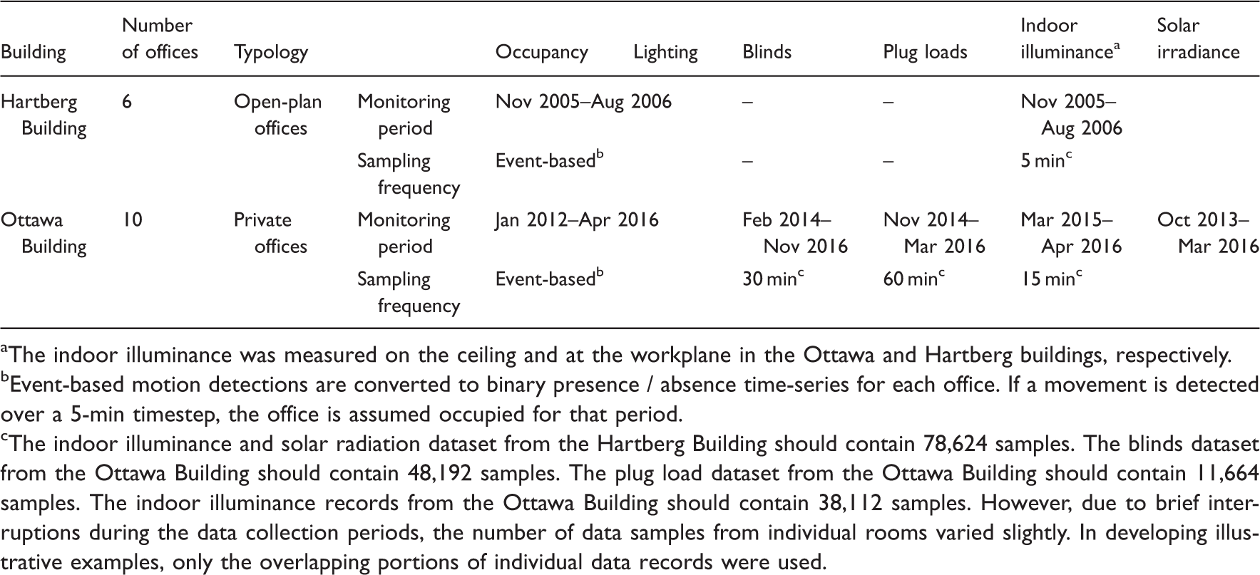
To develop illustrative examples, we used occupant behavior (for lighting, blinds, and plug-in equipment use) and occupancy data gathered from two office buildings. The buildings are located in Ottawa, Canada and Hartberg, Austria. The photos of the buildings are shown in Figure 1. Table 1 presents an overview of the characteristics of the data used in the illustrative examples. It is worth mentioning that the data logging frequencies and duration of data collection were chosen based on the requirements to capture variations in observations to develop statistically representative occupant models. For instance, using low frequencies of data logging can capture occupants' interactions with window shades as previous studies showed that occupants change shade positions very infrequently.^50,51 Data logging frequencies should also be high enough to capture changes in building systems and components to connect them with the influential parameters. On the other hand, the data storage capacity and battery life of stand-alone data loggers impose limitations on choosing the sampling and logging frequency. For instance, in the current research, the illuminance sensors/loggers were set to sample and log the data at the low temporal resolution of 15 min to balance the practicality of minimizing researcher visits to the offices with modelling needs. Therefore, it is preferable to use a network of sensors connected with building automation systems where researchers seek to record data at high frequencies for a long-term data collection study.

Figure 1.

The buildings from which the datasets were collected (left, Hartberg Building, right, Ottawa Building). The dotted lines enclose the windows of the rooms studied in this paper.

Table 1.

Overview of the datasets from the two case studies.

Building	Number of offices	Typology		Occupancy	Blinds	Plug loads	Indoor illuminance^a	Solar irradiance
Hartberg Building	6	Open-plan offices	Monitoring period	Nov 2005–Aug 2006	–	–	Nov 2005– Aug 2006
Hartberg Building	6	Open-plan offices	Sampling frequency	Event-based^b	–	–	5 min^c
Ottawa Building	10	Private offices	Monitoring period	Jan 2012–Apr 2016	Feb 2014– Nov 2016	Nov 2014– Mar 2016	Mar 2015– Apr 2016	Oct 2013– Mar 2016
Ottawa Building	10	Private offices	Sampling frequency	Event-based^b	30 min^c	60 min^c	15 min^c

The indoor illuminance was measured on the ceiling and at the workplane in the Ottawa and Hartberg buildings, respectively.

Event-based motion detections are converted to binary presence / absence time-series for each office. If a movement is detected over a 5-min timestep, the office is assumed occupied for that period.

The indoor illuminance and solar radiation dataset from the Hartberg Building should contain 78,624 samples. The blinds dataset from the Ottawa Building should contain 48,192 samples. The plug load dataset from the Ottawa Building should contain 11,664 samples. The indoor illuminance records from the Ottawa Building should contain 38,112 samples. However, due to brief interruptions during the data collection periods, the number of data samples from individual rooms varied slightly. In developing illustrative examples, only the overlapping portions of individual data records were used.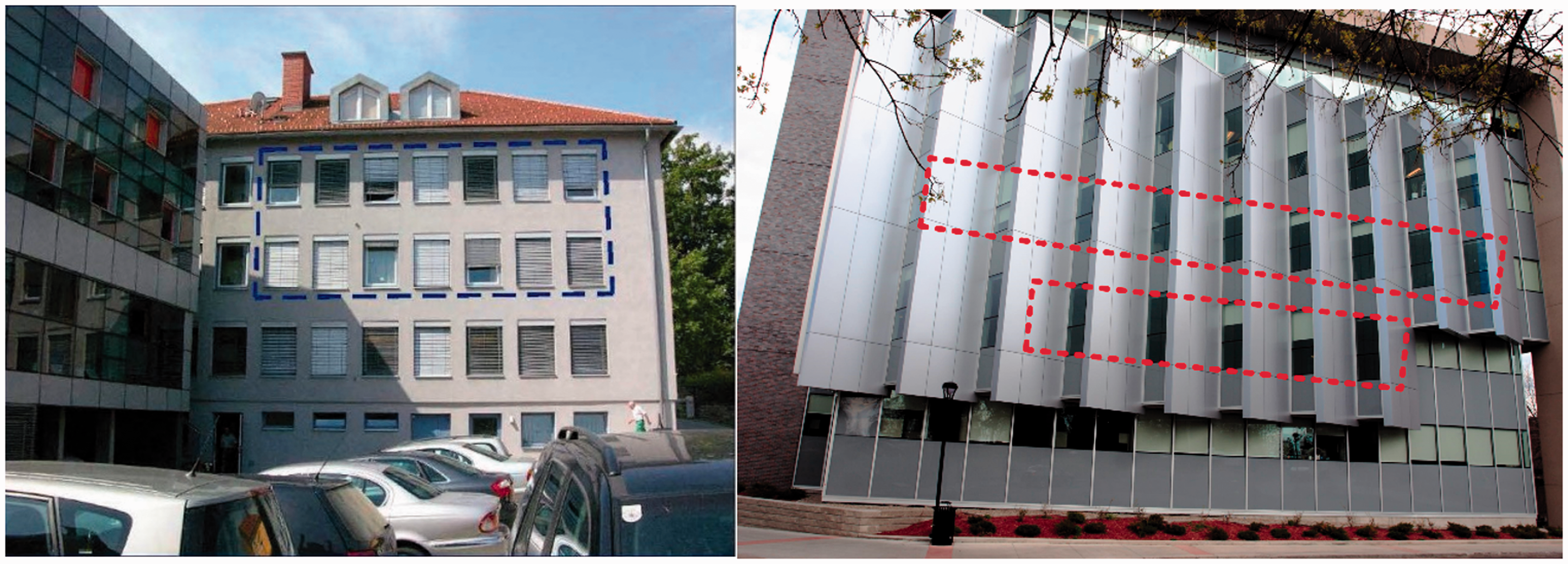

The exterior windows of the monitored offices are Northeast-facing in the Hartberg Building and West-facing in the Ottawa Building. The window-to-wall and window-to-floor ratios are 32% and 34% in the monitored offices in the Ottawa Building, and they are 24% and 18% in the Hartberg Building, respectively. The visible transmittance is 70% in the Ottawa Building offices, whereas it is 75% in the Hartberg office building. The occupants of the Ottawa Building were full-time faculty members in a university, and they were full-time municipal employees in a government building in the Hartberg Building. Further details about the data can be found elsewhere.^20,52,53

Modelling adaptive behaviors

In the reviewed literature, five different adaptive behavior model forms were found: (1) schedules, (2) Bernoulli models, (3) discrete-time Markov models, (4) discrete-event Markov models, and (5) survival models.

Schedules

The traditional way of modelling adaptive behaviors is schedules (e.g. presenting the ratio of the lights on or the mean blind occlusion rate averaged over a week or a month).⁵⁴ Figure 2 presents the mean weekday lighting schedule for the two datasets and the lighting schedules used in the archetype office buildings.⁵⁵ The data points in the plots represent the mean value by the time of day across weekdays that can be calculated as follows:

\bar{R} (l i g h t) = 1, T i m e = h = \frac{\sum^{​} N [l i g h t = 1 \land T i m e = h]}{\sum^{​} N [T i m e = h]}

(1)

where

\bar{R}

is the mean hourly lights on ratio, N is the timestep, light is the light state at each timestep (i.e. one represents lights on and zero lights off), and Time (h) is the time of day at each timestep. The numerator represents the number of timesteps when lights were on at a specific time of day. The denominator represents the number of timesteps at the considered time of day (h).

Figure 2.

Lighting use schedule for weekdays in the two office buildings and ASHRAE Standard 90.1.⁵⁵

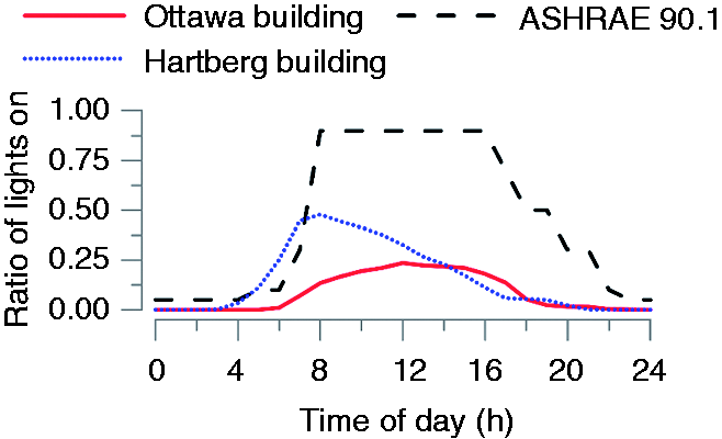
As illustrated in Figure 2, this approach provides information that is easy to interpret and does not require data from indoor environmental quality sensors. This model form is established based on the assumption that the time of the week or the month of the year alone is adequate to make predictions for occupant behaviors. This steady-periodicity is based on the assumption that either adaptive behaviors or predictor variables are cyclical.

However, because of the fixed nature of the schedule approach, schedules cannot be used to assess the impact of new building design on comfort-related triggers of behaviors – particularly for buildings that are significantly different than the buildings from which the schedules are based on. For example, changing the glazing material and geometry, shading material and controls, and lighting fixture and controls will affect the daylight availability, thereby playing a role in occupants' use of electric lighting. Because schedules do not incorporate indoor environmental proxies (e.g. workplane illuminance) to explain occupant behaviors, these models may fail to replicate adaptive actions effectively (e.g. for façade design)⁷ even if they are used in the cases where all contextual factors (e.g. building specifications and participants' characteristics) are similar to the context that the schedules were derived from. In addition, as they are deterministic, they fail to represent the inherent randomness in occupants' behaviors.

Bernoulli models

Another common method employed in adaptive behavior modelling is the Bernoulli random processes.^56,57 Bernoulli models predict the likelihood of finding a building component with which occupants interact at a given state (i.e. a window open or closed, lights on or off). Each scatter point in Figure 3 presents the ratio of the occupied duration when the lights were on to the occupied duration at varying solar irradiance levels. For example, the probability of finding the lights on when the incident solar irradiance on the façade is less than 50 W/m² is 0.72 in the Ottawa building while it is 0.74 when the horizontal solar irradiance is less than 50 W/m² in the Hartberg building. Each scatter point in Figure 3 can be represented in the following functional form:

\begin{array}{l} p (l i g h t = 1, Q_{s o l} = x) \\ = \frac{{\begin{cases} \sum^{​} N [o c c = 1 \land l i g h t = 1 \land (Q_{s o l} > (x - Δ x) \land \\ Q_{s o l} < (x + Δ x))] \end{cases}}}{\sum^{​} N [o c c = 1 \land (Q_{s o l} > (x - Δ x) \land Q_{s o l} < (x + Δ x))]} \end{array}

(2)

where p represents the probability of finding the lights on at a specific incident solar irradiance, N represents the timestep, occ is the occupancy at each time step (i.e. one represents presence and zero absence), light is the light state at each timestep, and Q_sol (W/m²) is the solar irradiance at each timestep. The variable x is a constant representing the solar irradiance level at which we intend to calculate the probability of finding the lights on. The variable Δx is a small constant relative to the full range of the predictor (Q_sol). The numerator can be interpreted as the sum of the occupied durations when the lights were on and solar irradiance was about x (W/m²). The denominator can be interpreted as the sum of the occupied durations when the solar irradiance was about x (W/m²).

Figure 3.

Bernoulli models predicting the fraction of the occupied period with lights on as a function of the solar irradiance in the Ottawa and Hartberg buildings. Solar irradiance values represent the incident solar irradiance on the façade of the Ottawa building and the horizontal solar irradiance for the Hartberg building.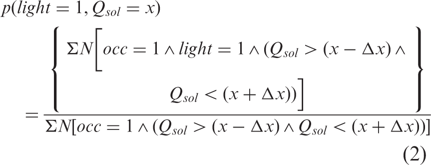

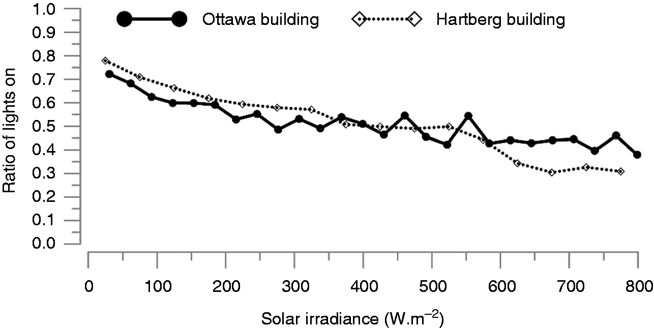
Occupants' adaptive actions are predictable with discomfort proxies (e.g. workplane illuminance is a predictor for insufficient daylight levels). However, reversal of an adaptive action (i.e. blinds opening or light switch off) can happen long after the discomfort conditions disappear.^58–62 As a result, the environmental predictors in Bernoulli models often cannot explain a significant variation in the occupants' control over building components. For instance, as presented in Figure 3, even when the solar irradiance reaches its upper limits, a considerable portion of the lights remained on in both buildings – meaning that users in these perimeter spaces do not actively adjust their blinds to exploit daylighting potential to replace electric lighting use. Similarly, the blind occlusion rate exhibits an insignificant variation as a function of the incident solar irradiance on the façade of the Ottawa building – as shown in Figure 4.

Figure 4.

A Bernoulli model predicting the blinds occlusion rate as a function of the solar irradiance in the Ottawa building.

Although Bernoulli occupant models have been developed with both indoor and outdoor explanatory variables in the literature,^8,56 these models are more appropriate to be used with outdoor variables.⁶³ This is because the adaptive behaviors trigger changes in the indoor environment, which contains both the predictor and the response variables. For example, the ratio of lights on when the workplane illuminance is less than 500 lux would be zero, if the electric lighting can provide at least 500 lux at the workplane when it is switched on. However, this means that Bernoulli occupant models are unsuitable for studying the impact of any building design features (e.g. window or shading geometry) that impact indoor conditions and corresponding comfort-related occupant behaviors.

Moreover, the advantages of developing models with outdoor variables instead of indoor variables (e.g. indoor illuminance and operative temperature) are the reduction in the cost of sensors and data collection, and the reduced risk of gathering biased information due to the Hawthorne effect.^37,64,65 As noted above, the major weakness of the Bernoulli models is that even if they are used in other buildings with comparable characteristics, they neglect the influence of differences in buildings' designs on occupants' adaptive actions. Similarly, they cannot be used to evaluate the impact of different building designs because of the relationship between outdoor conditions and those experienced by the occupants (i.e. indoor conditions) is design-specific.

Discrete-time Markov models

The third method used in modelling adaptive behaviors is the discrete-time Markov chains.^{41,61,62,66–69} The discrete-time Markov models predict the likelihood of undertaking an adaptive behavior in the next timestep. They can be developed by indoor and/or outdoor environmental variables because they are derived from the conditions just before occupants undertake the action. The Markov models treat adaptive actions and their reversals independently and have been suggested to predict behavior patterns more realistically. However, a common issue regarding the discrete-time Markov models is their dependency on fixed timesteps.⁷⁰ They only provide the likelihood of an occupant action in the next timestep. The fixed timestep concept implies that the frequency of an occupant's instances of decision-making remains constant, while it is logical that these cases increase in frequency during periods in which environmental conditions rapidly change (e.g. at arrival).

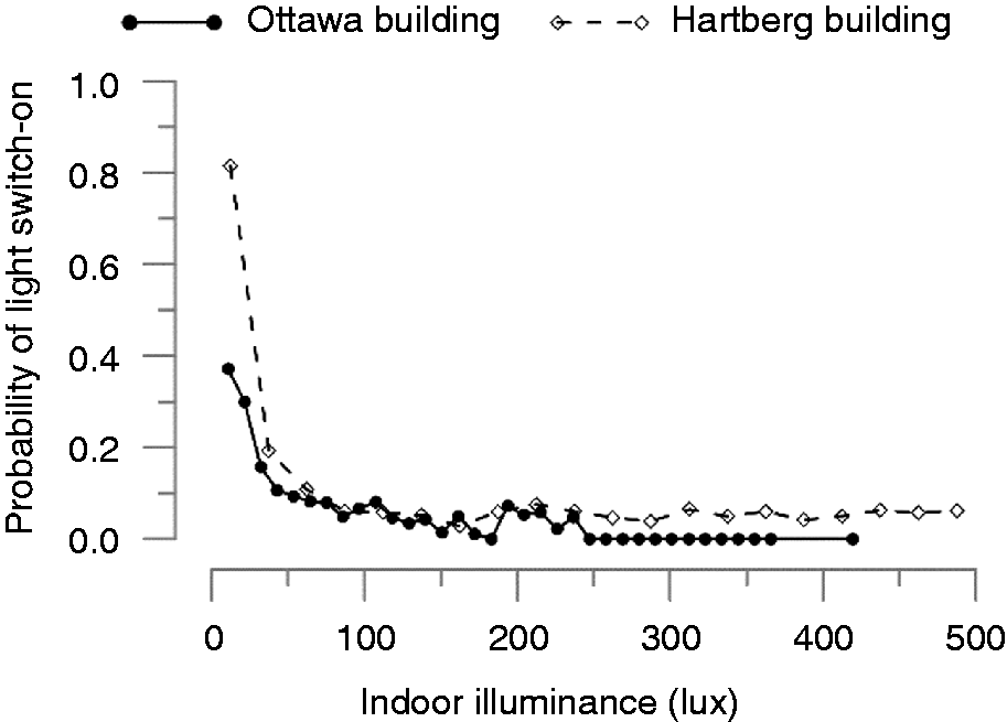
Figure 5 presents two discrete-time Markov models predicting the likelihood of a light switch-on action in the next 15 min for the Ottawa and Hartberg buildings. The scatter points represent the ratio of occupied timesteps with a light switch-on action to the total number of occupied timesteps when lights were off at a particular indoor illuminance level. To calculate the discrete likelihood values, the total number of occupied timesteps when the lights were off was grouped from all occupants at each bin. Bins were 25 lux for the Hartberg and 10 lux for the Ottawa building. Some of these timesteps were followed by a light switch-on action, while some were not. The ratio of those timesteps that led to a light switch-on action to the total occupied timesteps with lights off provides the likelihood of observing the light switch-on action in the next timestep. As shown in Figure 5, this ratio is significantly higher when the indoor illuminance levels are less than 50 lux. Each scatter point in Figure 5 can be represented in the following functional form:

\begin{array}{l} p (l i g h t = 1, E_{l u x} = x) \\ = \frac{{\begin{cases} \sum^{​} N [o c c = 1 \land s w i t c h_o n = 1 \land \\ (E_{l u x} > (x - Δ x) \land E_{l u x} < (x + Δ x))] \end{cases}}}{{\begin{cases} \sum^{​} N [o c c = 1 \land l i g h t = 0 \land \\ (E_{l u x} > (x - Δ x) \land E_{l u x} < (x + Δ x))] \end{cases}}} \end{array}

(3)

where N represents the timesteps, E_lux (lux) is the indoor illuminance at each timestep. The variable x is a constant representing the indoor illuminance level at which the probability of a light switch-on action is calculated. The variable Δx is a small constant relative to the full range of the predictor (E_lux). The numerator can be interpreted as the number of occupied timesteps with a light switch-on action when the indoor illuminance was about x (lux). The denominator can be interpreted as the number of occupied timesteps when the lights were off and the indoor illuminance was about x (lux). Note the relationship of the calculated probabilities to the timestep size.

Figure 5.

Discrete-time Markov models predicting the likelihood of a light switch-on action in the next 15 min as a function of the indoor illuminance. In the Ottawa building, the indoor illuminance measurements were taken on the ceiling and, they were taken at the workplane in the Hartberg building.

Discrete-event Markov models

Discrete-event Markov models link an occupant action to an external event.^57,61,62,71 For example, in Reinhart's⁶¹ light switch model implies that occupants are more likely to turn on their lights at arrivals (event). In Rijal et al.'s,⁶² occupants were modelled to consider window opening and closing upon a change in the predicted mean vote (event). Similarly, Gunay et al.⁷² treated discrete events for the light switch-on behavior as a change larger than 100 lux in the workplane illuminance levels.

When relevant events triggering the behavioral adaptation of the occupants can be identified, the models' predictive accuracy is shown to improve in contrast to discrete-time Markov models.⁷² However, the discrete-event Markov modelling approach is challenged by finding an appropriate event triggering the occupant's action, to replace the timestep concept – particularly with regards to integration in BPS tools. Another limitation of this method is that its predictive performance relies on the accuracy of the external events' predictions. For example, the predictive performance of Reinhart's⁶¹ discrete-event Markov light switch model will depend on our ability to detect the intermediate arrival and departure events accurately.

Figure 6 presents two discrete-event Markov models predicting the likelihood of a light switch-on action at arrival (including the first and intermediate arrivals) for the Ottawa and Hartberg buildings. The scatter points represent the ratio of arrival timesteps with a light switch-on action to the total number of arrival timesteps at a particular indoor illuminance level. To compute the discrete likelihood values, the total number of arrival events when the lights were off was grouped from all occupants at each bin (25 lux for the Hartberg and 10 lux for the Ottawa building). Some of these arrivals were followed by a light switch-on action, while some others were not. The ratio of arrivals that result in a light switch-on action to the total arrival timesteps with lights off provides the likelihood of observing the light switch-on action in the timestep right after the arrival. Each scatter point in Figure 6 can be represented in the following functional form:

\begin{array}{l} p (s w i t c h - o n = 1, E_{l u x} = x) \\ = \frac{{\begin{cases} \sum N [a r r = 1 \land s w i t c h - o n = 1 \land \\ (E_{l u x} > (x - Δ x) \land E_{l u x} < (x + Δ x))] \end{cases}}}{{\begin{cases} \sum N [a r r = 1 \land l i g h t = 0 \land \\ (E_{l u x} > (x - Δ x) \land E_{l u x} < (x + Δ x))] \end{cases}}} \end{array}

(4)

where arr is an array containing the arrival data records (e.g. one for a timestep with an arrival and otherwise zero). The variable x is a constant representing the indoor illuminance level at which the probability of a light switch-on action is calculated. The variable Δx is a small constant relative to the full range of the predictor (E_lux). The numerator can be interpreted as the number of arrivals with a light switch-on action when the indoor illuminance was about x (lux). The denominator can be interpreted as the number of arrivals when the lights were off and the indoor illuminance was about x (lux).

Figure 6.

Discrete-event Markov model predicting the likelihood of a light switch-on action at arrival as a function of the indoor illuminance. The illuminance readers were taken on the ceiling in the Ottawa building and workplane in the Hartberg building; thus, the results cannot be directly compared.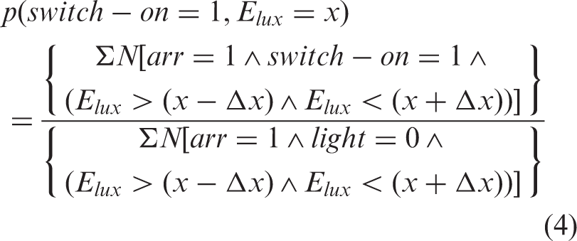

Survival models

The fifth method used in modelling adaptive behaviors is the survival models. The survival models found in the reviewed literature predict the lifetime of an occupant action or the state of a building component with which occupants interact. Examples of this model type were used in modelling blinds,^{21,61,66,73–75} operable windows,^1,66,69 and lighting.⁶¹ When survival models were used in modelling operable window use, the survival curve was modified as a function of indoor environmental variables. For example, in Haldi and Robinson's⁶⁶ window use model, the lifetime of a window position is predicted by a survival model which is a function of the indoor temperature. The limitation of this approach is that if the indoor environmental variable used in the model (e.g. indoor temperature) changes after making a prediction (e.g. a lifetime of a window's position), the duration predicted by the initial survival model will become unrepresentative.

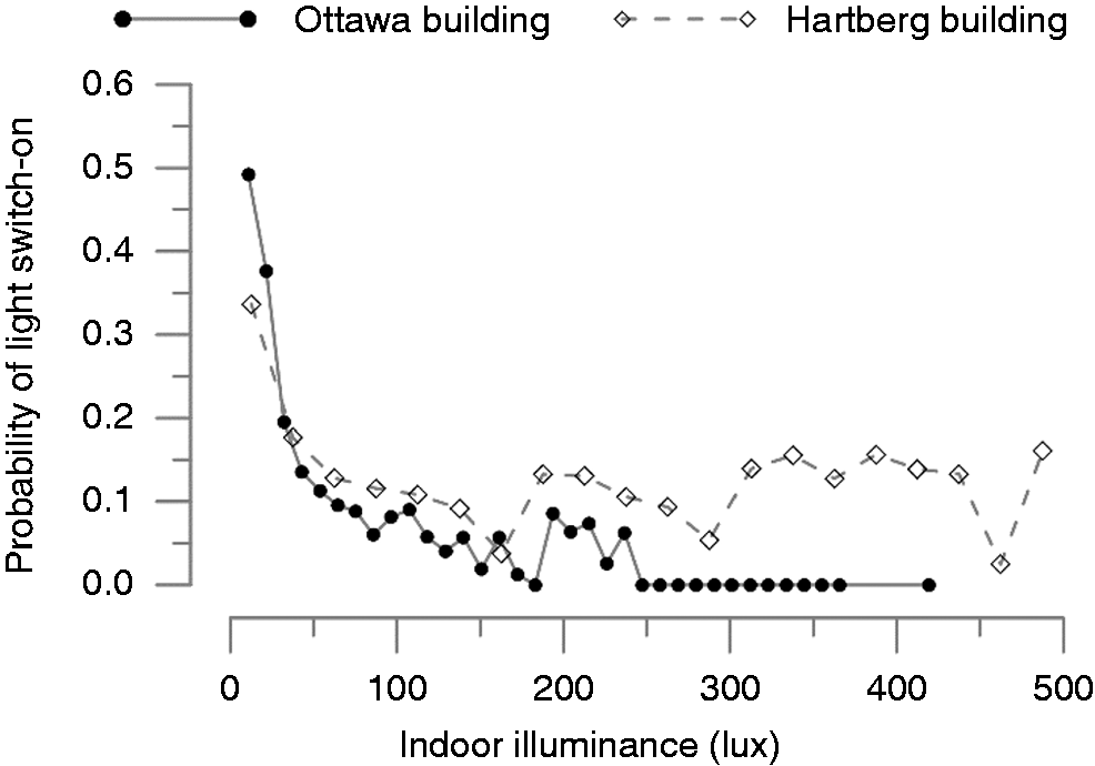
Based on the Ottawa Building, Figure 7 presents a survival model predicting the time between consecutive blind closing and opening actions as follows:

\begin{array}{l} p (b l i n d o p e n i n g = 1, t_{d u r a t i o n} = x) \\ = \frac{{\begin{cases} \sum^{​} N [b l i n d o p e n i n g = 1 \land \\ (t_{d u r a t i o n} > (x - Δ x) \land t_{d u r a t i o n} < (x + Δ x))] \end{cases}}}{\sum^{​} N [b l i n d o p e n i n g = 1]} \end{array}

(5)

where p is the probability of blind opening action for the duration of x (days) between consecutive blind closing and opening actions and

t_{duration}

is the duration between consecutive blind closing and opening actions. Δx is a small constant relative to the full-range of

t_{duration}

. The numerator indicates the number of blind opening actions when the duration of the consecutive blind opening and closing actions was x. The denominator indicates the number of the blind opening actions at the full range of

t_{duration}

. The results in Figure 7 indicate that in 30% of the cases it takes more than a week to reopen the blinds once they are closed. This observation is in line with the literature that the users' blind opening behavior is quite infrequent.¹⁵

Figure 7.

Survival models consecutive blinds closing and opening actions.

Regression methods for adaptive behavior models

The discrete likelihood weights in adaptive behavior models (e.g. see Figures 3 to 6) are often fitted as regression models to represent the information of the model with a number of parameter coefficients and to regularize them as continuous distributions.

In the reviewed literature on adaptive behavior modelling, two regression methods were found: (1) linear regression (e.g. linear or polynomial regression)^51,59,76,77 and (2) generalized linear regression (e.g. logistic, probit regression).^{56,62,66,69,78–84}

The shortcoming of linear regression is that it is not appropriate for probabilistic models where the response variables are bound between zero and one (e.g. probability). Thus, the generalized linear regression has become the de facto standard in adaptive behavior modelling.¹ It employs a nonlinear link function (e.g. probit or logit) to map the explanatory variables (e.g. indoor temperature) onto bounded response variables (e.g. the probability of observing a thermostat override). By employing the maximum likelihood method, one can develop the generalized linear models. Statistical packages for established programming environments provide built-in functions to develop generalized linear models (e.g. statsmodels in Python, glmfit or fitglm in Matlab, glm in R-programming).

Figure 8 presents a logistic regression fit for the discrete-time Markov light switch-on model for the Ottawa building. The areas of the bubble plots in Figure 8 indicate the observed occupancy duration when lights were off at each ceiling illuminance level. Note that the occupied durations are not homogeneously distributed at each illuminance level. Thus, an important consideration for building generalized linear models is to ensure that a representative number of observations is acquired from a wide-range of predictor conditions (e.g. monitoring light switch behavior from zero to 1000 lux on the workplane, monitoring thermostat use behavior from indoor air temperatures between 18 and 27 ℃).

Figure 8.

Probability of switching on the lights in the next 15 min (discrete-time Markov) in the Ottawa Building. The univariate logistic regression model is in the following form: 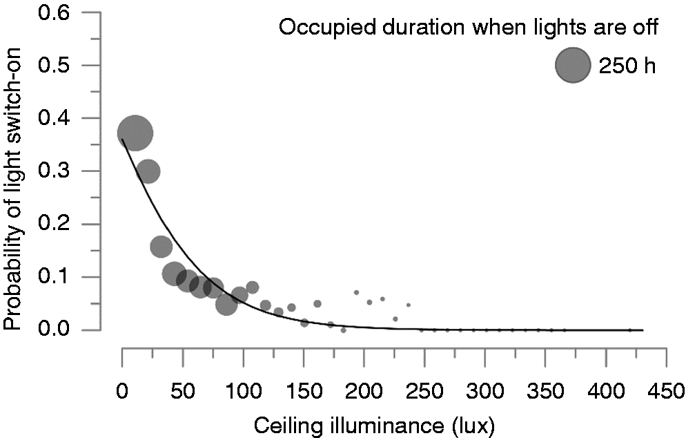$p = 1 / (1 + e^{- (a + b E_{lux})})$ .

The regression models can be univariate, where the model is fitted with respect to a single predictor (e.g. predicting the blind closing action with the workplane illuminance), or multivariate where the model is fitted with respect to two or more predictors (e.g. predicting the blind closing action with the workplane illuminance and indoor temperature). As mentioned in Haldi and Robinson,¹ increasing the number of predictors will provide diminishing improvements in the predictive accuracy. In addition, when there are many predictor candidates available and some of these variables exhibit multicollinearity, the modelers may need to employ an exhaustive model selection approaches such as the forward or backward stepwise regression or all-possible regressions. Alternatively, dimensionality reduction techniques which map the predictors to a lower dimensional space (e.g. the principal component analysis) can be used in predictor selection. For example, assume that a window use model is developed for indoor and outdoor temperatures, indoor relative humidity, wind-speed, indoor CO₂ concentration, and occupant clothing insulation levels. Most of these variables tend to exhibit pairwise correlation amongst each other. As outdoor temperatures get colder, the indoor humidity levels and indoor temperatures tend to decrease and occupant clothing insulation levels tend to increase. As a result, it is likely adequate to use only a subset of these predictor variable candidates. Detailed information about selecting top predictor variables that can provide the highest of predictive accuracy can be found elsewhere.⁸⁵

A cross-validation approach should be employed for the evaluation of the regression models.^66,69,86 If a model is not overfitted, the models developed upon training sets would be in agreement with the models developed upon the data retained for validation. Alternatively, the relative model quality can be assessed by computing the Akaike or the Bayesian Information Criteria. For example, Figure 9 contrasts the quality of two univariate logistic regression models (discrete-time and discrete-event Markov models) for the same dataset from the Ottawa building. By examining the Akaike Information Criterion values (smaller values are favorable), the discrete-time model appears to be a relatively better model for the dataset. Another commonly used metric for the assessment of the regression models is the coefficient of determination (R-squared). Note that for binomial data, ordinary R-squared should not be used. In that case, modelers should use pseudo R-squared values to assess the fitness of the model. Readers can refer to McCullagh and Nelder⁸⁷ for further information on generalized linear model development, selection, and validation procedures.

Figure 9.

Probability of switching on the lights in the next 15 min (discrete-time Markov) upon arrival (discrete-event Markov) in the Ottawa Building. The univariate logistic regression model is in the following form: 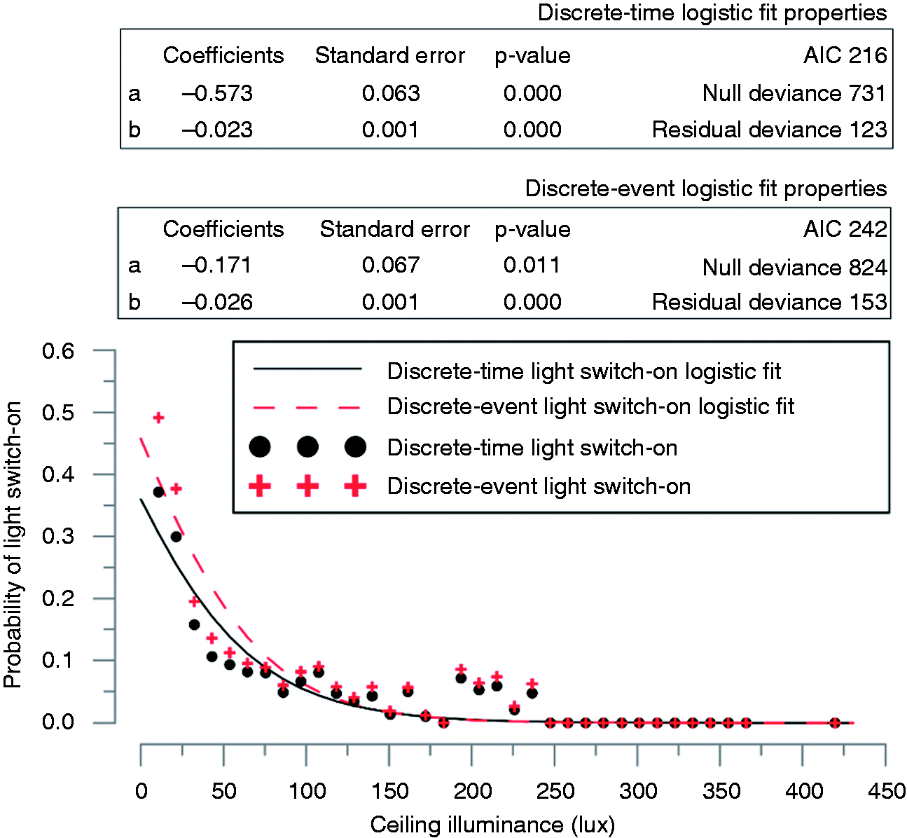$p = 1 / (1 + e^{- (a + b E_{lux})})$ . The properties of the regression parameters are annotated in the figure.

Modelling non-adaptive behaviors

Non-adaptive behaviors such as plug-in appliance use, light switch off or window closing at the time of departure are driven primarily by factors other than physical discomfort. Recall that non-adaptive behaviors are considered those which are not undertaken to improve comfort; instead they may be undertaken with motives such as saving energy, improving views to outside, and engaging in a task. In the reviewed literature, three modelling methods were identified for non-adaptive behavior modelling: (1) building schedules (e.g. Masoso and Grobler⁸⁸ and Menezes et al.⁸⁹), (2) using the occupancy schedule as the predictor,^26,90 and (3) constructing survival models.^75,91

Schedules

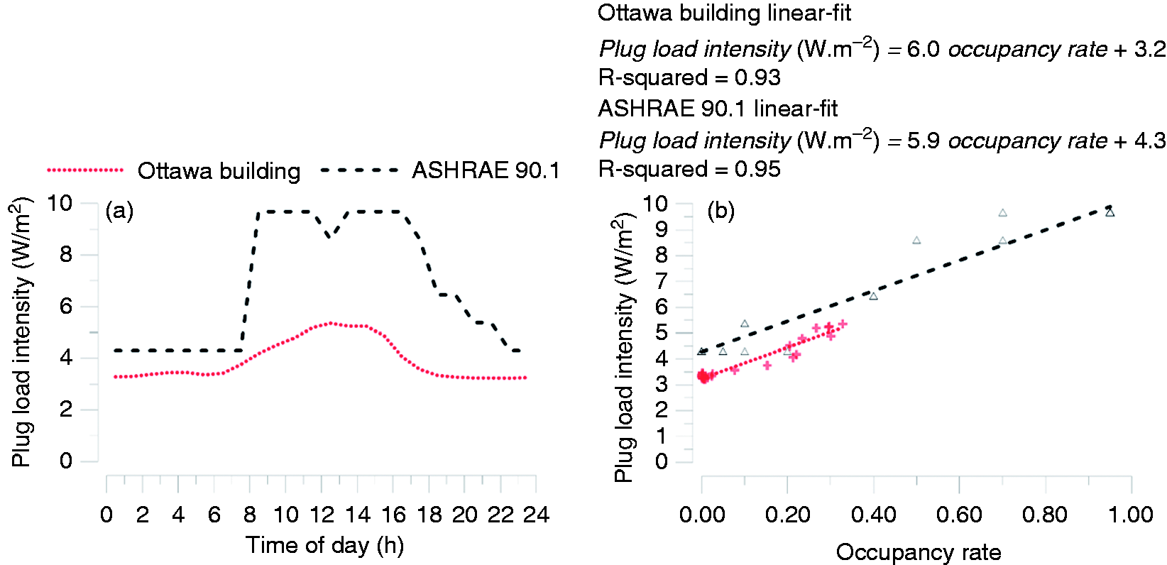
Similar to the adaptive behaviors, the traditional way of modelling non-adaptive occupant behaviors is using daily or weekly schedules. This method can be appropriate for modelling the non-adaptive occupant behaviors if they were developed from a similar building archetype.⁹² For example, Figure 10(a) presents the mean weekday plug-in appliance load intensity in the Ottawa building. While developing Figure 10(a) the hourly plug load data from individual offices were averaged across about 120 measurements taken at a given hour of any weekday. Similar to the lighting schedules shown in Figure 2, the data points in the plots shown in Figure 10(a) represent the mean value by the time of day across weekdays calculated using equation (6):

\bar{I} (T i m e = h) = \frac{\sum_{T i m e = h} I}{\sum^{​} N [T i m e = h]}

(6)

where

\bar{I}

is the mean daily plug-in appliance load intensity (W/m²) and I is the plug-in appliance load intensity (W/m²) at each timestep. The numerator represents the sum of plug-in appliance load intensity at all the timesteps when the time of day is h. The denominator represents the number of timesteps for each time of the day. Note that the Ottawa building had substantially different plug-in equipment schedules from the ASHRAE Standard 90.1⁵⁵ reference office building (Figure 10(a)), largely because of the low occupancy.

Figure 10.

The average plug-in appliance load intensity on a weekday in the Ottawa building as (a) a schedule and (b) its relationship with the mean occupancy rate.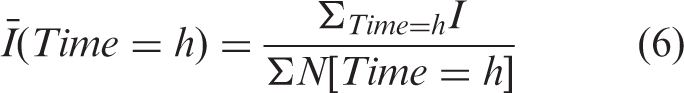

Occupancy schedules

Using the occupancy schedule as a predictor is another model form found in the reviewed literature for the non-adaptive behavior modelling.^90,93 The low-occupancy Ottawa office building and the ASHRAE Standard 90.1⁵⁵ reference office building appeared to have similar plug-in appliance load intensities when they were normalized with the occupancy rate (see Figure 10(b)). Similarly, Mahdavi et al.⁹⁰ developed a new model predicting the plug-in equipment power using the mean occupancy rate.

Survival models

The third method used in modelling non-adaptive behaviors is the survival models. The survival models found in the reviewed literature predict the likelihood of a light switch off action at departure, as a function of the duration of absence following the departure.^21,26,94 In a similar fashion, the plug-in appliance load intensities during vacancy periods were modelled as a function of the duration of vacancy period.²⁰ The survival models exploit the availability of matching occupancy data to elaborate the relationship between the non-adaptive behaviors and the occupancy/vacancy state, albeit with the added complexity to collect concurrent occupancy data.

Figure 11 presents two survival models of non-adaptive behavior built upon the data gathered from the Ottawa building. The first example (Figure 11(a)) presents the ratio of departures with a manual light switch off action to the total number of departures when the lights were on prior to departure as a function of the duration of absence. This model can be represented in the following functional form:

\begin{array}{l} p (s w i t c h - o f f = 1, t_{d u r a t i o n} = x) \\ = \frac{{\begin{cases} \sum^{​} N [s w i t c h - o f f = 1 \land \\ (t_{d u r a t i o n} > (x - Δ x) \land t_{d u r a t i o n} < (x + Δ x))] \end{cases}}}{{\begin{cases} \sum^{​} N [l i g h t = 1 \land (t_{d u r a t i o n} > (x - Δ x) \\ \land t_{d u r a t i o n} < (x + Δ x))] \end{cases}}} \end{array}

(7)

where p is the probability of light switch-off actions at departure duration of x (day), t_duration is the duration between consecutive departure and arrival. Δx is a small constant relative to the full-range of t_duration. The numerator indicates the number of light switch-off actions when the duration of the consecutive departure and arrival was x. The denominator indicates the number of timesteps when lights were on and the consecutive departure and arrival was x. The results indicate that in almost 70% of the cases, the users left their dimmable and motion detector-automated artificial lighting on (with a 30-min delay) during intermediate breaks. Pigg et al.⁹⁵ similarly found a large fraction of occupants leaving lights on upon departure in offices with vacancy-off lighting controls.

Figure 11.

Different survival models built upon the data gathered from the Ottawa building: (a) likelihood of a light switch off at departure as a function of the duration of absence, and (b) plug-in appliance load intensity during vacancy as a function of the duration of absence.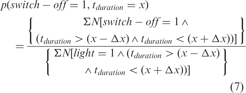

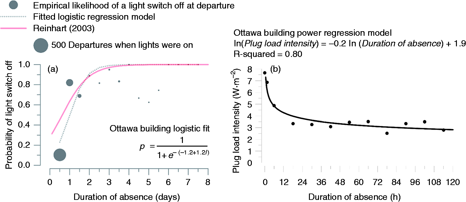
The second example (Figure 11(b)) presents the plug-in appliance load intensities during vacancy periods as a function of the duration of the absence. The model was established upon the mean plug load values at varying durations of absence. The scatter points represent the mean plug load measured at different periods of occupancy/vacancy – in 12 h bins – computed as follows:

\begin{array}{l} \bar{I} (d u r a t i o n = x) \\ = \frac{\sum^{​} [I a t (t_{d u r a t i o n} > (x - Δ x) \land t_{d u r a t i o n} < (x + Δ x))]}{\sum^{​} N [(t_{d u r a t i o n} > (x - Δ x) \land t_{d u r a t i o n} < (x + Δ x))]} \end{array}

(8)

where

\bar{I}

is the mean plug-in appliance load intensity (W/m²) at vacancy duration of x (h), t_duration is the duration of vacancy. Δx is a small constant relative to the full-range of vacancy. The numerator indicates the sum of plug-in appliance load intensity at all the timesteps when the vacancy duration was x. The denominator indicates the number of timesteps when the vacancy duration was x. Note that a commonly used performance metric for the evaluation of linear regression models is R-squared as a measure of how well a model can predict the measured data (see Figures 10(b) and 11(b)). The results, as shown in Figure 11(b), indicate that the mean plug-in equipment load per occupant was about 8 W.m⁻² during occupancy, and it decreased to 3 W.m⁻² during absences longer than three days. This can be interpreted as occupants' tendency to turn off their plug-in equipment increases as a function of the duration of their absence. The model mimics this behavior through a regression model in which the mean plug load exponentially reduces as a function of the length of absence.

Modelling presence

As occupants' behaviors are conditional upon their presence, it is essential to understand and characterize the randomness inherent in occupants' presence patterns to represent their behaviors realistically. In modelling presence in buildings, three different methods have been typically used: (1) schedules,^24,96 (2) discrete-time Markov models,^25,97,98 and (3) survival models.⁹⁹

Occupancy schedules

The most common occupancy modelling method is building weekly occupancy schedules – presenting the ratio of presence as a function of the time of day and day of the week.^100,101 Figure 12 presents the ASHRAE Standard 90.1 (2013) and the weekday occupancy schedule in the two office buildings of this paper calculated based on equation (9):

\bar{O c c} (o c c = 1, T i m e = h) = \frac{\sum^{​} N [o c c = 1 T i m e = h]}{\sum^{​} N [T i m e = h]}

(9)

where

\bar{Occ}

is the mean hourly occupancy ratio, N is the timestep, Occ is the occupancy at each timestep (i.e. one represents presence and zero absence), and Time (h) is the time of day at each timestep. The numerator represents the number of timesteps when occupants were present at a specific time of day. The denominator represents the number of timesteps at the considered time of day (h).

Figure 12.

Occupancy schedule for weekdays in the two office buildings and ASHRAE Standard 90.1.⁵⁵

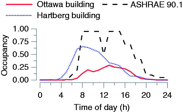
The results indicate that the occupancy in the Hartberg building peaks in the morning, whereas the occupancy in the Ottawa building peaks in the afternoon. The occupancy rates in the Ottawa building – an academic office building used by professors – were noticeably lower than the Hartberg building – a government building used by municipal employees. However, the occupancy rates in both buildings were substantially lower than those of ASHRAE Standard 90.1.⁵⁵

The advantage of this model form is that it is easy to interpret by building operators and control technicians. Moreover, it is suitable for large building scales (i.e. office floors, schools, entire large buildings).¹⁰² Building specific occupancy schedules provides valuable insights that can help operators choose operating schedules. Simulation experts can incorporate them quickly into building models to represent occupancy. However, schedules do not provide a discrete number of occupants nor do they directly predict individual arrival and departure events, as is often required for predicting adaptive actions (see Section “Modelling adaptive behaviors”). Page et al.⁴ and Mahdavi and Tahmasebi²⁸ introduced a method to generate occupancy data (i.e. sequential presence and absence information) from an occupancy schedule.

Discrete-time Markov models

The second method used in occupancy modelling is the Markov chains.^4,25 These models predict the likelihood of an arrival when occupants are absent, and it predicts the probability of a departure when occupants are present. For example, Figure 13 presents discrete-time Markov models predicting the likelihood of observing a first arrival or a last departure in the next hour based on the two example datasets (Harberg and Ottawa buildings). The models were built by computing the ratio of the number of first arrivals (last departures) to the total number of unoccupied duration (occupied duration) at a certain hour of a weekday. Each scatter point in Figure 13 can be represented in the functional form described in equation (10):

\begin{array}{l} p (a r r = 1, t_{d a y} = x) \\ = \frac{\sum N [a r r = 1 \land (t_{d a y} > (x - Δ x) \land t_{d a y} < (x + Δ x))]}{\sum N [o c c = 0 \land (t_{d a y} > (x - Δ x) \land t_{d a y} < (x + Δ x))]} \end{array}

(10)

where t_day (h) is an array of the time of day for each timestep in the dataset. The variable x is a constant representing the time of day for which the probability of an arrival event is calculated. The variable Δx is a small constant relative to the full range of the predictor (t_day). The numerator can be interpreted as the number of timesteps with an arrival event when the time of day was about x. The denominator can be interpreted as the number of unoccupied timesteps when the time of day was about x.

Figure 13.

Discrete-time Markov models providing the likelihood of observing a first arrival or a last departure in the next hour on a weekday.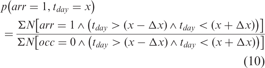

The results shown in Figure 13 indicate the occupants in the Hartberg building tend to arrive earlier and leave later than the occupants of the Ottawa building. The occupants' first arrival and last departure distributions exhibit a rather weak bimodality in the Ottawa building; meaning that occupants' first arrivals may take place in the afternoon, or their last departures can occur in the morning. This type of behavior was not observed in the Hartberg building. The strength of this approach – unlike the traditional schedule-based models – lies in the fact that the likelihood of observing an arrival or a departure from the rest of the day can be estimated given current time and the current state of presence. This may help to make midday control decisions such as temperature setbacks when the likelihood of observing an arrival is too small for the rest of the day.¹⁰³ The Markov occupancy models are also capable of creating realistic occupancy time-series which can be used in BPS models.⁹⁶ A weakness of the Markov occupancy models is that they treat arrival and departure events independently. In reality, occupants may depart early when they arrive early, or they may depart late when they arrive late.¹⁰⁴

Survival models

Survival occupancy models predict the duration of an intermediate vacancy period following a departure or they can predict the length of an intermediate occupancy period upon an arrival.⁹⁹ Note that the term intermediate vacancy period represents a coffee or a lunch break during a workday. The term intermediate occupancy period represents an occupied period between a consecutive arrival and departure. Figure 14 presents survival models predicting the duration of an uninterrupted intermediate occupancy or vacancy period for the two example datasets (Hartberg and Ottawa building). It is built upon the distribution of the duration of individual occupancy or vacancy periods. For example, more than 30% of the recorded intermediate vacancy periods exceeded 1.5 h in the Hartberg building. In contrast, this was about 2.5 h in the Ottawa building. Similarly, 30% of the uninterrupted intermediate occupancy periods were longer than 1 h in the Hartberg building. This was about 2 h in the Ottawa building. Therefore, the occupants of the Ottawa building tend to stay in their offices for longer periods without taking breaks. However, their intermediate breaks tend to persist longer than those in the Hartberg building.

Figure 14.

Survival models predicting the duration of an intermediate vacancy or presence period.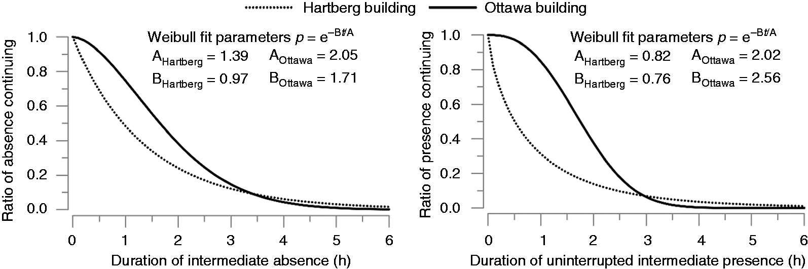

Discussion

The modelling methods discussed in this paper have different strengths and weaknesses, many of which are dependent on the application case (e.g. code compliance vs. design-oriented modelling). Based on the literature review, issues encountered through the illustrative examples, and the authors' experience, the following section provides a summary of the occupant model forms with regard to their use cases (Section “Use cases for occupant behavior modelling approaches”), as well as their strengths and weaknesses (Section “Strengths and weaknesses of occupant behavior modelling approaches”). Unresolved modelling issues and future requirements are discussed in Section “Unresolved modelling issues and future requirements”.

Use cases for occupant behavior modelling approaches

Some of the inappropriate use cases found in the literature – which the authors suggest should be avoided in future research and development – can be listed as follows:

Schedules and Bernoulli models for adaptive behaviors should not be used in comparing design alternatives because such models generally do not use indoor conditions as predictors for behavior.⁷ For example, changing the window-to-wall ratio and presence of fixed shading devices will influence the users' lighting and blind use behaviors.^105,106

Bernoulli models should not be developed with indoor environmental variables affected by the behavior (e.g. developing Bernoulli lighting use models with workplane illuminance data or developing Bernoulli window use models with indoor temperature data).^56,72 For example, when the lights are switched on in a typical office environment, the workplane illuminance would not fall below 300–500 lux. As a result, the model predictions for the ratio of lights on become dependent on the lighting state rather than workplane illuminance. Note that this is not an issue for the Markov models as they use the conditions immediately before the adaptive actions take place.

Discrete-time Markov models predict the likelihood of an occupant action in the next timestep.⁹¹ Model coefficients are sensitive to the timestep length; modelers must report the timestep size that they use.

Discrete-event Markov models predict the likelihood of an occupant's action at an event instance. Modelers should define these event steps in which the occupant models will be invoked, and then insure they are implemented in the simulation phase. Some early examples of occupant models found in the reviewed literature (e.g. Hunt¹⁰⁷) did not report when these models should be called during simulation.

Survival models are best suited to non-adaptive behavior modelling, though they may be used for modelling adaptive behavior. However, this approach is more appropriate in infrequently executed adaptive behaviors, such as the blinds use behavior. For example, when Haldi and Robinson⁶⁶ developed survival models to predict the duration windows remain open, they had to vary the survival curves for different indoor and outdoor temperatures because the window closing behavior is influenced by the indoor and outdoor temperatures. Given that the indoor and outdoor temperatures can change substantially in time, the opening durations predicted by the survival model can become inappropriate before the predicted opening period elapses.

Strengths and weaknesses of occupant behavior modelling approaches

Some of the strengths and weaknesses of occupant behavior modelling approaches are listed as follows:

The main advantage of using schedules for occupant modelling is the ease of development and application to a range of adaptive behaviors and building archetypes. The strength of this model form is that only a single data type (the model output itself) is necessary to build it and it is easy to interpret for building operators and energy modelers. For this reason, schedules have been extensively used in BPS practice and introduced as recommendations in the design standards and codes (e.g. ASHRAE⁵⁵ and NRC¹⁰⁸). This model form is established based on the assumption that the time of the week or the month of the year alone is adequate to make predictions for the occupant behavior and presence. However, the fixed nature of schedules means than any design features or control strategies aimed at changing behavior cannot be evaluated.

Bernoulli processes provide some improvement (over schedules) in explaining occupants' adaptive behaviors with environmental explanatory variables. The limitation of Bernoulli processes is that these models are developed based on observations of a building component's state (e.g. window position), not the actual interactions with it (e.g. window opening or closing). Thus, these models do not describe the probability of window opening or closing, but the likelihood for a window to be found open, as a function of predictor variables. In some applications, designers may wish to predict the number of actions (e.g. as a proxy for comfort), which is not possible with Bernoulli processes.

Discrete-time Markov models have become popular among the research community because of the straightforwardness of pairing consecutive probabilities of occupants' actions with some simulated changes in environmental conditions. In general, Markov models fit simulation processes in BPS tools in the format of discrete timesteps. However, in reality occupants' adaptive action events take place at irregular time intervals. In such view, discrete-time Markov models may fail to capture behavior patterns. As an example, occupants tend to close their blinds when the indoor illuminance is changing – not when it remains constant over time. Discrete-time Markov occupancy models can represent the frequency and timing of the arrivals and departures. However, the major drawback of using this form for occupancy modelling is that the consecutive arrival and departure events are treated independently from each other.

Discrete-event Markov models link the calling points of an occupant action model to an external event. This modelling approach may address some of the limitations of the aforementioned methodologies. It is, however, challenged by finding an appropriate event definition to replace the timestep concept. Another limitation of this approach is that its predictive performance relies on the accuracy of the external events' predictions.

Survival models predict the duration that an occupant interacting system's state remains unchanged. They overcome the issue that discrete-time Markov occupancy models may fail to capture potential dependencies between arrival and departure events by relating the timing of these events to each other. For example, after a departure event, a survival model may predict the duration of a vacancy or break period. However, because they are continuous-time random processes, the rounding errors can be significant when used with large timesteps in BPS.

Unresolved modelling issues and future requirements

With the objective to strive for widespread and accurate occupant modelling to support better building designs, it is crucial to develop and apply the best model(s) that can reproduce the relationship between occupants and the predictor variables. Depending on criteria such as model purpose, modeler experience, and building type, modelers should strive for occupant models to achieve a compromise between the complexity and accuracy. An occupant model should characterize the observed occupant behavior patterns by looking at a small set of explanatory variables that are isolated from the many possible indoor and outdoor environmental indicators and other predictors.

In response to pervasive sensing and data archiving solutions in buildings, in recent years, machine learning-based occupant modelling formalisms have also begun emerging. For instance, previous research used machine learning techniques to predict occupancy^109–111 and occupants' interactions with buildings^112–115 and energy use.¹¹⁶ These techniques are particularly beneficial in modelling with large datasets regarding occupant–building interactions. Machine learning techniques also draw a promising future in building operations as occupant feedback can be integrated in the control loop using such algorithms in building automation systems.^117–119 However, machine learning techniques often lack the transparency of the regression models presented in this paper. While the need for professionals with the knowledge and skills of machine learning techniques is growing for studying occupants in building performance analysis, simplification of the machine learning-based occupant modelling techniques is also necessary for their use by the industry. Moreover, it is critical that model users understand the occupant models and their underlying assumptions; adding complexity poses a risk to this matter. For instance, machine learning features can be integrated within BPS tools. Emerging algorithms in machine learning, such as unsupervised learning (aka self-learning), without requiring training outputs based on inputs, also encourage researchers to use these techniques in studying occupants in buildings.^120–122 For instance, self-adaptive occupant models can be developed for building control. Moreover, providing comprehensive documentations of monitored cases and developing well-established structures for consistent and informative data collection and management¹²³ are required to improve models' reproducibility.

Further, as a result of several recent comparative studies,^54,124 it has become clear that occupant models that are developed for one building may not be used in others due to building-specific contextual factors and peculiarities.¹⁸ Another largely unresolved issue, which is aimed to be answered in the new International Energy Agency – Energy in Buildings and Communities (IEA-EBC) Annex 79 on “Occupant-centric building design and operation”, is combining multiple occupant models in a single simulation. The reviewed articles mainly focused on developing occupant models for a single application domain (e.g. light use behavior or occupancy) and did not explore their compatibility with other models. There are logistical issues, such as the fact that some adaptive action models require models that predict occupant arrival. However, there are also strong interactions between behaviors that are not readily addressed in the literature. For example, an occupant in a dark office may choose to open blinds or turn on lights (or both) to resolve the issue. In reality, this decision-making process is complex and involves considerations of ease, energy cost, comfort, longevity, and effectiveness of the adaptive measure. In a building model, however, the modelled decision may merely depend on the order in which the models are called during a particular simulation time step.

One area of future investigation is to develop integrated occupant models that consider comfort requirements, behavioral actions, psychological, physiological, and sociological factors altogether. These domains are currently implicitly considered in an unintegrated way to some extent. Greater modelling capability and accuracy would be afforded by an interdisciplinary occupant modelling approach going further.

Some adaptive actions are undertaken infrequently such as changing blind position.¹ Consequently, it becomes very expensive (and time-consuming) to gather an adequate dataset. This burden raises the question of whether or not having a dynamic adaptive behavioral model for some domains is practical for building energy simulation purposes.

Conclusions

In this paper, the occupant modelling methodologies from the literature were reviewed for the purpose of critically assessing them as well as for pedagogical benefit for researchers and advanced industry-based modelers. Further, illustrative occupant models were developed using two independent datasets from an academic office building in Ottawa, Canada and a government building in Hartberg, Austria. Based on the review of the literature and the analyses of these datasets, the strengths, weaknesses, and use cases of each model form were identified.

This paper categorized the occupant models into three groups: (1) adaptive behavior models, (2) non-adaptive behavior models and (3) occupancy models. Adaptive behavior models use environmental explanatory variables such as illuminance level, indoor and outdoor temperature, to predict occupants' actions primarily undertaken to restore occupant comfort (e.g. light switch-on, blinds closing, thermostat use, window use, and clothing adjustments). The non-adaptive behaviors are actions mainly driven by contextual factors, rather than physical discomfort (e.g. plug-in appliance use, light switch off when leaving the space).

In the reviewed literature, the adaptive behavior models were developed as weekly schedules, Bernoulli models, discrete-time and discrete-event Markov models, and survival models. Bernoulli models predict the likelihood of finding a building component with which occupants frequently interact at a given state (e.g. ratio of lights on at a certain outdoor illuminance level). Markov models predict the likelihood of an adaptive action as a function of explanatory variables (e.g. the probability of a light switch-on in the next timestep for the discrete-time Markov models or in the next event step such as at the next arrival for the discrete-event Markov models). Survival models predict the timing of the next adaptive action through random sampling from an empirical probability distribution (e.g. a lifetime of a blind position before it is changed). Adaptive behavior models are often fitted as regression models to regularize the parameter coefficients representing the model as continuous distributions.

Non-adaptive behavior models have been developed as weekly schedules, survival models, or by using the occupancy schedules from a similar building. The survival models predict the timing of the next non-adaptive action (e.g. likelihood of a light switch-off or the probability of computer switch-off action at departure).

Occupancy models have been developed as weekly schedules, discrete-time Markov models predicting the timing and frequency of the arrivals or departures, and survival models predicting the duration of an uninterrupted occupancy or vacancy period.

Outcomes of the literature review and illustrative examples demonstrated that Markov models are best suited to represent occupants' adaptive behaviors, while survival models are appropriate to represent occupancy, non-adaptive behaviors, as well as infrequently executed adaptive behaviors, such as the blinds opening behavior.

Footnotes

Declaration of conflicting interests

The author(s) declared no potential conflicts of interest with respect to the research, authorship, and/or publication of this article.

Funding

The author(s) acknowledge the generous funding from Natural Resources Canada and project partners RWDI, Autodesk, and National Research Council of Canada.

References

Haldi

Robinson

. The impact of occupants' behaviour on building energy demand. J Build Perform Simul 2011; 4: 323–338.

Norford

Socolow

Hsieh

, et al. Two-to-one discrepancy between measured and predicted performance of a ‘low-energy’ office building: insights from a reconciliation based on the DOE-2 model. Energy Build 1994; 21: 121–131.

Yan

O'Brien

Hong

, et al. Occupant behavior modeling for building performance simulation: current state and future challenges. Energy Build 2015; 107: 264–278.

Page

Robinson

Morel

, et al. A generalised stochastic model for the simulation of occupant presence. Energy Build 2008; 40: 83–98.

O'Brien

Gunay

. Mitigating office performance uncertainty of occupant use of window blinds and lighting using robust design. Build Simul 2015; 8: 621–636.

Fadzli Haniff

Selamat

Yusof

, et al. Review of HVAC scheduling techniques for buildings towards energy-efficient and cost-effective operations. Renew Sustain Energy Rev 2013; 27: 94–103.

Hoes

Hensen

JLM

Loomans

MGLC

, et al. User behavior in whole building simulation. Energy Build 2009; 41: 295–302.

Nicol

Humphreys

. A stochastic approach to thermal comfort–occupant behavior and energy use in buildings. ASHRAE Trans 2004, pp. 110: 554–568, .

Borgeson S and Brager G. Occupant control of windows: accounting for human behavior in building simulation. UC Berkeley: Center for the Built Environment, https://escholarship.org/uc/item/5gx2n1zz (accessed 23 January 2019).

10.

Fabi

Andersen

Corgnati

, et al. A methodology for modelling energy-related human behaviour: application to window opening behaviour in residential buildings. Build Simul 2013; 6: 415–427.

11.

Schiavon

Lee

. Dynamic predictive clothing insulation models based on outdoor air and indoor operative temperatures. Build Environ 2013; 59: 250–260.

12.

Morgan

de Dear

. Weather, clothing and thermal adaptation to indoor climate. Clim Res 2003; 24: 267–284.

13.

Nicol

Humphreys

. Adaptive thermal comfort and sustainable thermal standards for buildings. Energy Build 2002; 34: 563–572.

14.

Newsham

. Clothing as a thermal comfort moderator and the effect on energy consumption. Energy Build 1997; 26: 283–291.

15.

Gunay

O'Brien

Beausoleil-Morrison

. A critical review of observation studies, modeling, and simulation of adaptive occupant behaviors in offices. Build Environ 2013; 70: 31–47.

16.

Schweiker

Carlucci

Andersen

, et al. Occupancy and occupants' actions. In: Wagner A, O Brien W and Dong B (eds) Exploring occupant behavior in buildings 2018 Berlin: Springer, pp. 7–38. .

17.

Sadeghi

Karava

Konstantzos

, et al. Occupant interactions with shading and lighting systems using different control interfaces: a pilot field study. Build Environ 2016; 97: 177–195.

18.

O'Brien

Gunay

. The contextual factors contributing to occupants' adaptive comfort behaviors in offices – a review and proposed modeling framework. Build Environ 2014; 77: 77–87.

19.

Menezes

Cripps

Buswell

, et al. Estimating the energy consumption and power demand of small power equipment in office buildings. Energy Build 2014; 75: 199–209.

20.

Gunay

O'Brien

Beausoleil-Morrison

, et al. Modeling plug-in equipment load patterns in private office spaces. Energy Build 2016; 121: 234–249.

21.

Pigg S, Eilers M and Reed J. Behavioral aspects of lighting and occupancy sensors in private offices: a case study of a university office building. In: ACEEE 1996 summer study on energy efficiency in buildings. Pacific Grove, CA, 25-31 August 1996, pp.161–170.

22.

D'Oca

Hong

. Occupancy schedules learning process through a data mining framework. Energy Build 2015; 88: 395–408.

23.

Tahmasebi

Mostofi

Mahdavi

. Exploring the implications of different occupancy modelling approaches for building performance simulation results. Energy Proc 2015; 78: 567–572.

24.

Duarte

Van Den Wymelenberg

Rieger

. Revealing occupancy patterns in an office building through the use of occupancy sensor data. Energy Build 2013; 67: 587–595.

25.

Wang

Yan

Jiang

. A novel approach for building occupancy simulation. Build Simul 2011; 4: 149–167.

26.

Mahdavi A and Pröglhöf C Toward empirically-based models of people's presence and actions in buildings. In: Eleventh International IBPSA Conference, Glasgow, Scotland, 27-30 July 2009, pp. 537–544.

27.

Langevin J, Wen J and Gurian PL. Including occupants in building performance simulation: integration of an agent-based occupant behavior algorithm with Energy Plus. In: ASHRAE/IBPSAUSA building simulation conference, Atlanta, GA, 10-12 September 2014.

28.

Mahdavi

Tahmasebi

. Predicting people's presence in buildings: an empirically based model performance analysis. Energy Build 2015; 86: 349–355.

29.

Dong B and Andrews B. Sensor-based occupancy behavioral pattern recognition for energy and comfort management in intelligent buildings. In: Eleventh International IBPSA Conference, Glasgow, Scotland, 27-30 July 2009, pp. 1444–1451.

30.

Dong B and Lam KP. A real-time model predictive control for building heating and cooling systems based on the occupancy behavior pattern detection and local weather forecasting. Build Simul 2014; 7(1): 89–106.

31.

Beltran A and Cerpa AE. Optimal HVAC building control with occupancy prediction. In: Proceedings of the 1st ACM conference on embedded systems for energy-efficient buildings, Memphis, TN, 5-6 November 2014, pp. 168–171. New York: ACM.

32.

Zeiler W, Labeodan T and Boxem G. Detecting and tracing building occupants to optimize process control. In: Proceedings of the 14th International Conference on Enhanced Building Operations, Beijing, China, 14-17 September 2014, pp. 1–9.

33.

Zhao

Lam

Ydstie

, et al. Occupant-oriented mixed-mode EnergyPlus predictive control simulation. Energy Build 2016; 117: 362–371.

34.

Yan

Hong

Dong

, et al. IEA EBC Annex 66: definition and simulation of occupant behavior in buildings. Energy Build 2017; 156: 258–270.

35.

Gaetani

Hoes

P-J

Hensen

JLM

. Occupant behavior in building energy simulation: towards a fit-for-purpose modeling strategy. Energy Build 2016; 121: 188–204.

36.

Yang

Santamouris

Lee

. Review of occupancy sensing systems and occupancy modeling methodologies for the application in institutional buildings. Energy Build 2016; 121: 344–349.

37.

Gilani

O'Brien

. Review of current methods, opportunities, and challenges for in-situ monitoring to support occupant modeling in office spaces. J Build Perform Simul 2017; 10: 444–470.

38.

Fabi

Andersen

Corgnati

, et al. Occupants' window opening behaviour: a literature review of factors influencing occupant behaviour and models. Build Environ 2012; 58: 188–198.

39.

O'Brien

Kapsis

Athienitis

. Manually-operated window shade patterns in office buildings: a critical review. Build Environ 2013; 60: 319–338.

40.

Dong B, Yan D, Li Z, et al. Modeling occupancy and behavior for better building design and operation—a critical review. Build Simul 2018; 11(5): 899–921.

41.

Hong

Taylor-Lange

D'Oca

, et al. Advances in research and applications of energy-related occupant behavior in buildings. Energy Build 2016; 116: 694–702.

42.

Hong

Sun

Chen

, et al. An occupant behavior modeling tool for co-simulation. Energy Build 2016; 117: 272–281.

43.

Ouf M, O'Brien W and Gunay B. Improving occupant-related features in building performance simulation tools. Build Simul 2018: 11(4): 803–817.

44.

Gunay

O'Brien

Beausoleil-Morrison

. A Critical review of state-of-the-art energy and comfort related occupant behavior in office buildings. Build Environ 2013; 70: 31–47.

45.

Haldi F. A probabilistic model to predict building occupants' diversity towards their interactions with the building envelope. In: 13th Conference of International Building Performance Simulation Association, Chambéry, France, 26-28 August 2013, pp. 1475–1482.

46.

Mahdavi A and Tahmasebi F. The inter-individual variance of the defining markers of occupancy patterns in office buildings: a case study. In: Proceedings of BS2015: 14th Conference of International Building Performance Simulation Association, Hyderabad, India, 7-9 December 2015, pp. 2243–2247.

47.

Tahmasebi

Mahdavi

. On the utility of occupants' behavioural diversity information for building performance simulation: an exploratory case study. Energy Build 2018; 176: 380–389.

48.

Haldi

Calì

Andersen

, et al. Modelling diversity in building occupant behaviour: a novel statistical approach. J Build Perform Simul 2017; 10: 527–544.

49.

O'Brien

Gunay

Tahmasebi

, et al. A preliminary study of representing the inter-occupant diversity in occupant modelling. J Build Perform Simul 2017; 10: 509–526.

50.

Rea

. Window blind occlusion: a pilot study. Build Environ 1984; 19: 133–137.

51.

Inoue

Kawase

Ibamoto

, et al. The development of an optimal control system for window shading devices based on investigations in office buildings. ASHRAE Trans 1988; 94: 1034–1049.

52.

Gunay HB, O'Brien W, Beausoleil-Morrison I, et al. Development and implementation of an adaptive lighting and blinds control algorithm. Build Environ 2016; 113: 185–199.

53.

Mahdavi

Mohammadi

Kabir

, et al. Occupants' operation of lighting and shading systems in office buildings. J Build Perform Simul 2008; 1: 57–65.

54.

Schweiker

Haldi

Shukuya

, et al. Verification of stochastic models of window opening behaviour for residential buildings. J Build Perform Simul 2012; 5: 55–74.

55.

ASHRAE. ANSI/ASHRAE/IES Standard 90.1-2013 – Energy standard for buildings except low-rise residential buildings. ASHRAE, Atlanta, GA, 2013.

56.

Haldi

Robinson

. On the behaviour and adaptation of office occupants. Build Environ 2008; 43: 2163–2177.

57.

Herkel

Knapp

Pfafferott

. Towards a model of user behaviour regarding the manual control of windows in office buildings. Build Environ 2008; 43: 588–600.

58.

Rubinstein

Ward

Verderber

. Improving the performance of photo-electrically controlled lighting systems. J Illuminat Eng Soc 1989; 18: 70–94.

59.

Foster

Oreszczyn

. Occupant control of passive systems: the use of Venetian blinds. Build Environ 2001; 36: 149–155.

60.

Sutter

Dumortier

Fontoynont

. The use of shading systems in VDU task offices: a pilot study. Energy Build 2006; 38: 780–789.

61.

Reinhart

. Lightswitch-2002: a model for manual and automated control of electric lighting and blinds. Solar Energy 2004; 77: 15–28.

62.

Rijal

Tuohy

Nicol

, et al. Development of an adaptive window-opening algorithm to predict the thermal comfort, energy use and overheating in buildings. J Build Perform Simul 2008; 1: 17–30.

63.

Gunay HB, O'Brien W and Beausoleil-Morrison I. A toolkit for developing data-driven occupant behaviour and presence models. In: eSim 2016, Hamilton, Ontario, 3-6 May 2016.

64.

Mahdavi

. People in building performance simulation. In: Hensen JLM and Lamberts R (eds). Building performance simulation for design and operation 2011, pp. 56–83. London: Routledge.

65.

Humphreys

Nicol

. Understanding the adaptive approach to thermal comfort. ASHRAE Trans 1998; 104: 991.

66.

Haldi

Robinson

. Interactions with window openings by office occupants. Build Environ 2009; 44: 2378–2395.

67.

Fritsch

Kohler

Nygård-Ferguson

, et al. A stochastic model of user behaviour regarding ventilation. Build Environ 1990; 25: 173–181.

68.

Lindelöf

Morel

. A field investigation of the intermediate light switching by users. Energy Build 2006; 38: 790–801.

69.

Haldi

Robinson

. Adaptive actions on shading devices in response to local visual stimuli. J Build Perform Simul 2010; 3: 135–153.

70.

Gunay

O'Brien

Beausoleil-Morrison

, et al. Coupling stochastic occupant models to building performance simulation using the discrete event system specification formalism. J Build Perform Simul 2014; 7: 457–478.

71.

Yun

Steemers

. Time-dependent occupant behaviour models of window control in summer. Build Environ 2008; 43: 1471–1482.

72.

Gunay HB, O'Brien W, Beausoleil-Morrison I, et al. On modelling and simulation of occupant models. In: Proceedings of BS2015: 14th Conference of International Building Performance Simulation Association, Hyderabad, India, 7-9 December 2015, pp. 1501–1508.

73.

Gunay

. Improving energy efficiency in office buildings through adaptive control of the indoor climate, Ottawa: Carleton University, 2016.

74.

Gunay

O'Brien

Beausoleil-Morrison

, et al. Implementation of an adaptive occupancy and building learning temperature setback algorithm. ASHRAE Trans 2016, pp. 122: 179–192, .

75.

Parys

Saelens

Hens

. Coupling of dynamic building simulation with stochastic modelling of occupant behaviour in offices – a review-based integrated methodology. J Build Perform Simul 2011; 4: 339–358.

76.

Inkarojrit V and Paliaga G. Indoor climatic influences on the operation of windows in a naturally ventilated building. In: 21th PLEA conference, Eindhoven, The Netherlands, 19-22 September 2004.

77.

Warren

Parkins

. Window-opening behaviour in office buildings. Build Serv Eng Res Technol 1984; 5: 89–101.

78.

Clarke J, Macdonald I and Nicol J. Predicting adaptive responses simulating occupied environments. In: Proceedings of international comfort and energy use in buildings conference. Network for Comfort and Energy Use in Buildings (NCEUB), London. 2006.

79.

Haldi

Robinson

. Modelling occupants' personal characteristics for thermal comfort prediction. Int J Biometeorol 2011; 55: 681–694.

80.

Inkarojrit

. Monitoring and modelling of manually-controlled Venetian blinds in private offices: a pilot study. J Build Perform Simul 2008; 1: 75–89.

81.

Nicol JF. Characterising occupant behaviour in buildings: towards a stochastic model of occupant use of windows, lights, blinds, heaters and fans. In: Proceedings of the seventh international IBPSA conference, Rio, Rio de Janeiro, Brazil, 13-15 August 2001, pp. 1073–1078.

82.

Rijal

Tuohy

Humphreys

, et al. Using results from field surveys to predict the effect of open windows on thermal comfort and energy use in buildings. Energy Build 2007; 39: 823–836.

83.

Zhang Y and Barrett P. Factors influencing the occupants' window-opening behaviour in a naturally ventilated office building. Build Environ 2012; 50: 125–134.

84.

Zhang

Barrett

. Factors influencing occupants' blind-control behaviour in a naturally ventilated office building. Build Environ 2012; 54: 137–147.

85.

Bishop

. Pattern recognition and machine learning, Berlin: Springer, 2006. .

86.

Mahdavi

Tahmasebi

. On the quality evaluation of behavioural models for building performance applications. J Build Perform Simul 2017; 10: 554–564.

87.

McCullagh

Nelder

. Generalized linear models, New York: CRC Press, 1989. .

88.

Masoso

Grobler

. The dark side of occupants' behaviour on building energy use. Energy Build 2010; 42: 173–177.

89.

Menezes AC, Cripps A, Buswell RA, et al. Benchmarking small power energy consumption in the United Kingdom: a review of data published in CIBSE Guide F. Build Serv Eng Res Technol 2012; 34(1): 73–86.

90.

Mahdavi

Tahmasebi

Kayalar

. Prediction of plug loads in office buildings: simplified and probabilistic methods. Energy Build 2016; 129: 322–329.

91.

Haldi F. Towards a unified model of occupants' behaviour and comfort for building energy simulation. PhD Thesis, EPFL, 2010.

92.

Deru M, Field K, Studer D, et al. US Department of Energy commercial reference building models of the national building stock. Technical Report, NREL/TP-5500-46861, National Renewable Energy Laboratory, Golden, Colorado, 2011.

93.

Mahdavi A and Pröglhöf C. User behavior and energy performance in buildings. Wien, Austria: Internationalen Energiewirtschaftstagung an der TU Wien (IEWT), 2009.

94.

Boyce

. Observations of the manual switching of lighting. Light Res Technol 1980; 12: 195–205.

95.

Chang

W-K

Hong

. Statistical analysis and modeling of occupancy patterns in open-plan offices using measured lighting-switch data. Build Simul 2013; 6: 23–32.

96.

Andersen

Iversen

Madsen

, et al. Dynamic modeling of presence of occupants using inhomogeneous Markov chains. Energy Build 2014; 69: 213–223.

97.

Parys W, Saelens D and Hens H. Implementing realistic occupant behavior in building energy simulations–the effect on the results of an optimization of office buildings. In: Proceedings of the 10th REHVA World Congress “Sustainable Energy use in Buildings, 2010, pp. 1–8.

98.

Wang

Federspiel

Rubinstein

. Modeling occupancy in single person offices. Energy Build 2005; 37: 121–126.

99.

Gunay

O'Brien

Beausoleil-Morrison

. Implementation and comparison of existing occupant behaviour models in EnergyPlus. J Build Perform Simul 2015; 9(6): 567–588. .

100.

Mahdavi

Tahmasebi

. The deployment-dependence of occupancy-related models in building performance simulation. Energy Build 2016; 117: 313–320.

101.

Gilani

O'Brien

Gunay

. Simulating occupants' impact on building energy performance at different spatial scales. Build Environ 2018; 132: 327–337.

102.

Gunay

O'Brien

Beausoleil-Morrison

. Development of an occupancy learning algorithm for terminal heating and cooling units. Build Environ 2015; 93: 71–85.

103.

Page J. Simulating occupant presence and behaviour in buildings. PhD Thesis, EPFL, 2007.

104.

Gilani

O'Brien

Gunay

, et al. Use of dynamic occupant behavior models in the building design and code compliance processes. Energy Build 2016; 117: 260–271.

105.

Sanati

Utzinger

. The effect of window shading design on occupant use of blinds and electric lighting. Build Environ 2013; 64: 67–76.

106.

Hunt

. The use of artificial lighting in relation to daylight levels and occupancy. Build Environ 1979; 14: 21–33.

107.

NRC. National energy code of Canada for buildings, Ottawa: National Research Council Canada, 2015. .

108.

Chen

Masood

Soh

. A fusion framework for occupancy estimation in office buildings based on environmental sensor data. Energy Build 2016; 133: 790–798.

109.

Candanedo

Feldheim

Deramaix

. A methodology based on hidden Markov models for occupancy detection and a case study in a low energy residential building. Energy Build 2017; 148: 327–341.

110.

Chen

Soh

. Comparing occupancy models and data mining approaches for regular occupancy prediction in commercial buildings. J Build Perform Simul 2017; 10: 545–553.

111.

Bonte M, Perles A, Lartigue B, et al. An occupant behavior model based on artificial intelligence for energy building simulation. In: Proceedings of the 13th international IBPSA conference BS2013, Chambery, France, 26-28 August 2014, pp. 1467–1474.

112.

Markovic

Wolf

Cao

, et al. Comparison of different classification algorithms for the detection of user's interaction with windows in office buildings. Energy Proc 2017; 122: 337–342.

113.

Markovic

Grintal

Wölki

, et al. Window opening model using deep learning methods. Build Environ 2018; 145: 319–329.

114.

D'Oca

Hong

. A data-mining approach to discover patterns of window opening and closing behavior in offices. Build Environ 2014; 82: 726–739.

115.

Khosrowpour

Gulbinas

Taylor

. Occupant workstation level energy-use prediction in commercial buildings: developing and assessing a new method to enable targeted energy efficiency programs. Energy Build 2016; 127: 1133–1145.

116.

Ortega JG, Han L, Whittacker N, et al. A machine-learning based approach to model user occupancy and activity patterns for energy saving in buildings. In: 2015 science and information conference (SAI), 2015, pp. 474–482. Piscataway, NJ: IEEE.

117.

Basnayake

Amarasinghe

Attalage

, et al. Artificial intelligence based smart building automation controller for energy efficiency improvements in existing building. Int J Adv Automat Sci Technol 2015; 40: 85–91. .

118.

Vázquez-Canteli

Nagy

. Reinforcement learning for demand response: a review of algorithms and modeling techniques. Appl Energy 2019; 235: 1072–1089.

119.

Miller

Nagy

Schlueter

. A review of unsupervised statistical learning and visual analytics techniques applied to performance analysis of non-residential buildings. Renew Sustain Energy Rev 2018; 81: 1365–1377.

120.

Kim

Zhou

Schiavon

, et al. Personal comfort models: predicting individuals' thermal preference using occupant heating and cooling behavior and machine learning. Build Environ 2018; 129: 96–106.

121.

Kim

Schiavon

Brager

. Personal comfort models – a new paradigm in thermal comfort for occupant-centric environmental control. Build Environ 2018; 132: 114–124.

122.

Mahdavi

Taheri

. An ontology for building monitoring. J Build Perform Simul 2017; 10: 499–508.

123.

Tahmasebi

Mahdavi

. An inquiry into the reliability of window operation models in building performance simulation. Build Environ 2016; 105: 343–357.