Estimating and mapping urban heat islands of the UK by interpolation from the UK Met Office observing network

Abstract

In this paper, we estimate the climatological impact of urbanisation in the UK as derived from the present and historical set of temperature observations from the UK network of meteorological observing stations. A well-established method for interpolation of in-situ temperature observations is used to make an estimate of temperatures at urban weather station locations based on rural climate data. This method avoids reliance on simple pairing of urban–rural stations commonly used for station-based analysis, and explicitly accounts for other topographic features such as elevation and coastal effects that will introduce geographical differences in temperature. The method is then applied to select a network of ‘rural’ weather stations deemed to be largely free from the direct influence of urban micro-climate effects. Comparison of the temperature grids derived from the ‘urban’ and ‘rural only’ station sets enables quantification of climatological urban heat island intensity across the UK and the influence on temperature in the UK national observational network observations from urban stations.

Practical application: This new method allows the estimation of the urban heat island for towns and cities of any size. Researchers will find it useful when making predictions of the urban heat island and of climate change in the urban environment, and when investigating morbidity and mortality due to overheating in buildings.

Keywords

Urban climate urban heat island weather data

Introduction

The urban heat island has long been recognised as a form of localised man-made climate change¹ as a consequence of the heat capacity, albedo, radiation trapping and local heat sources within the urban environment.² However, within Western Europe, most major towns and cities have been in existence for longer than we have had modern meteorological measurements. Therefore, we do not have climatological data for those locations as they would have been free from urban influence. Attempts to quantify urban heat islands therefore regularly rely on reference to the closest available rural sites,³ remote sensing,⁴ targeted observation campaigns^5,6 or with numerical climate models.^7,8

The consensus from this work is that urban heat islands are predominantly a nocturnal phenomenon with intensities up to 7°C in London (Watkins et al.⁵) and 10°C in Greater Manchester (Smith et al.⁶). The average rural–urban thermal contrast on summer night times was measured in Greater London as 2.71 ± 1.69°C⁵ and 5°C in Greater Manchester⁶ on nights with ideal UHI conditions. To consider the UHII in the design process, building designers can access empirical factors for design days (found in the CIBSE Guide A2 1⁷). These factors are relevant for June, July and August over London and Manchester. The factors are hourly with a maximum adjustment factor of 2.4°C and 6°C occurring at nightime at the city centres for London and Greater Manchester, respectively. The adjustments for London are considerably lower as they are relative to Heathrow which has its own UHI.

A systematic review of the international urban climate literature by Stewart⁹ found that nearly half of all published urban heat island magnitudes were scientifically indefensible, failing in particular to adequately control for the confounding effects of weather and topography. Near-neighbour comparisons can be problematic in this regard because our cities also tend to be located in strategically and geographically useful locations such as river valleys, estuaries, hilltops, or coastal sites that may also have climatological traits distinct from the wider surrounding area. So at least part of a cities micro-climate will also be a consequence of such geographical features. Satellite-based remote sensing can add valuable spatial detail, but can be limited by cloud cover and anisotropy of the urban landscape.¹⁰ Numerical modelling can add great value, but many assumptions about urban form are required and considerable development of urban land surface exchange schemes continues.¹¹

In this analysis, we provide a new assessment of UK urban heat islands with a blend of in situ surface observations and statistical models. The work has been conducted in order to contribute to a wider project exploring the potential impact of climate change on UK building design and energy use. The purpose of this contribution has been to develop a new methodology for creating urban and rural temperature climatologies for the UK based on the in situ network of meteorological observing stations spanning the period 1960 to 2015. In the previous work, Kershaw et al.¹² (2010, hereafter K10) developed a simple method to estimate urban heat island influence on gridded monthly near surface air temperature data (Perry and Hollis 2005b, hereafter PH05b¹³) spanning 1961–2006. Rather than relying on single site urban–rural temperature differences, K10 used the gridded datasets of temperature and urban land cover to evaluate temperatures within concentric circles around major urban centres in the UK and derive simple statistical model of urban heat island intensities. This has the advantage of using all available temperatures around the city, while minimising the influence of non-climatic factors. In this analysis, we improve on the K10 method in two key areas. Firstly, we adopt a more up-to-date and realistic urban land cover dataset which is at higher resolution and better resolves some of the inhomogeneities of the urban surface. Secondly, rather than trying to extract the urban signal from a single realisation of the PH05b¹³ gridded data, we produce a distinct version of the temperature grid derived solely from rural stations and interpolating across major urban areas. This new interpolation attempts to estimate a rural baseline reference temperature. The approach also allows for quantification of some of the key uncertainties outlined in K10.

Data and methods

Gridded datasets of maximum and minimum air temperature existed prior to this study, both for the 30-year average (Perry and Hollis 2005a, hereafter PH05a¹⁴) and for each individual day since 1 January 1960 (Perry, Hollis, and Elms 2009, hereafter PH09¹⁵). The gridding method used to create these datasets utilised regression analysis to model the relationship between temperature and topography and inverse-distance-weighted averaging to interpolate the regression residuals to a uniformly distributed set of points.

For the purposes of the current analysis, we have generated a version of the gridded datasets only using stations that display rural exposure characteristics, hereafter referred to as ‘rural only’. This re-gridding has also necessitated the regeneration of the existing gridded datasets referred to hereafter as the ‘all station’ set. This was done for two reasons – firstly, to ensure the ‘all station’ and ‘rural only’ versions of each grid were generated using a consistent approach, and secondly, to allow us to use new land cover datasets to characterise spatial variations in urban fraction.

Our starting point was the station averages for 1981–2010 that had been used to create the existing long-term average (LTA) grids of PH05a.¹⁴ Values were available for the mean daily maximum temperature and the mean daily minimum temperature. As part of the previous gridding work (PH05a¹⁴), these data underwent quality control checks to remove suspect values and a number of non-standard sites were also excluded. As well as UK stations, the input database also contained averages for stations in the Republic of Ireland – these had been incorporated by PH05a¹⁴ to improve the interpolation over Northern Ireland. In this analysis, we have used a UK only dataset of urban land use class and therefore have not classified the Irish stations as ‘urban’ or ‘rural’ and consequently these stations were not included. For the daily series, manual inspection and quality control were undertaken on the original PH09¹⁵ dataset. The set of quality control decisions were merged with complete data extracted from the Met Office Integrated Data Archive System (MIDAS, a version of which is available from Met Office, 2012¹⁶).

The interpolation process used to generate the gridded dataset is almost identical to that outlined in the references above. However, a further summary outlining key steps and model parameters where there are minor differences is provided as supplementary material. The primary differences within this analysis are that within the ‘rural’ station set, the urban land use component of the regression model is not used, and in the all station set, an updated urban land cover dataset has been adopted.

Defining urban land exposure for the UK observing network

The Centre for Ecology and Hydrology land cover map 2007¹⁷ has been used in this analysis, specifically v1.2 1 km percentage target class dataset. The land cover dataset distinguishes urban (U) and sub-urban (SU) land cover types. Using a geographic information system (GIS), both raster datasets were converted to 1 km polygons. Following McCarthy et al.,⁸ these two classes were combined to produce a single aggregated urban class (AU) where

AU = U + 0. 5 \times SU

Using these polygons, an AU percentage was extracted for the location of all UK meteorological observing stations that have contributed to the gridded temperature datasets.

A percentage AU cover within a 5 km radius of the site was also calculated. Selected examples of urban exposure are shown in Figure 1. Figure 1(1) is an example of a highly urban site and shows Camden Square, a historical urban station in central London, which has a 1 km AU and 5 km AU of 79%. Figure 1(2) shows Dyce, near Aberdeen which has a high 1 km AU of 80% but a low 5 km AU of 9%, reflecting its location on a built up airfield with otherwise rural surroundings. Figure 1(3) shows Pollock Country Park, which has a low 1 km AU of 10% but a higher 5 km AU of 45% due to the proximity of Glasgow. Figure 1(4) shows an example of the coastal site Southend which has a 1 km AU 76% and a 5 km AU of 21%. This last example is situation common to many stations located in or near the urban centre of UK coastal towns, whereby the 5 km urban statistics are moderated by the proximity to the “rural” sea.

Figure 1.

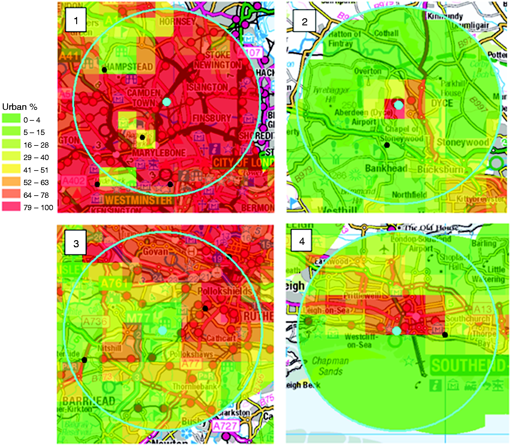
Examples of observing sites showing 1 km (squares) and 5 km (blue circle) AU. (1) Camden Square, London, (2) Dyce, Aberdeenshire, (3) Pollock country park, Glasgow, and (4) Southend, Essex. Colour scale shows aggregated urban class (AU, see text) as a percentage of total area of each 1 km grid square. Contains OS data © Crown copyright and database right (2018).

In preparing guidance on the siting of urban meteorological stations, Oke states that ‘There is no more important input to the success of an urban station than an appreciation of the concept of scale’.¹⁸ Oke¹⁸ describes micro-scale, local-scale and meso-scale factors. The conceptual model adopted within this project is framed around quantifying the manifestation of urban heat island effects at the regional and meso-scale, or city-scale, by making use of all available stations across the urban and surrounding environment. The results in this paper will be discussed in the context of a set of reasonably large metropolitan areas shown in Figure 2. The statistical modelling does not account for very localised effects. The identification of sites with relatively high 1 km AU means that we can identify and remove sites, such as Dyce, that may have local-scale urban bias from our set of rural sites, but it is the 5 km AU fraction that is the focus of the subsequent analysis and used within the interpolation scheme.

Figure 2.

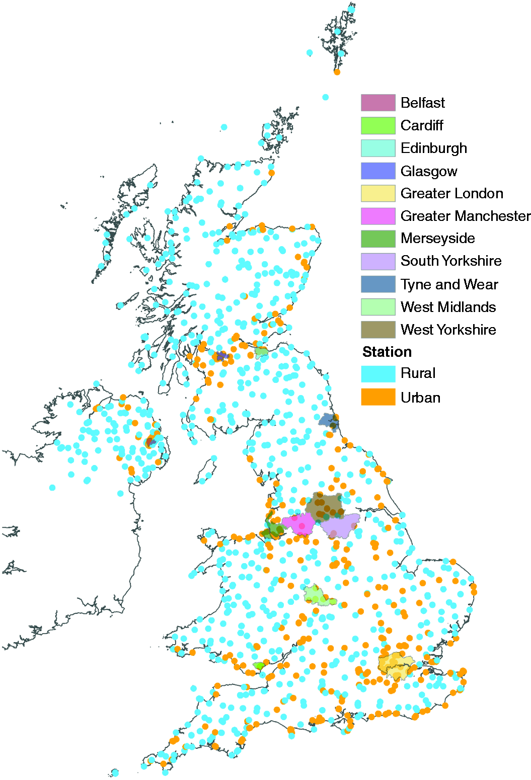
Map showing distribution of ‘rural only’ (blue) and urban (yellow) observing stations. Metropolitan areas used to analyse areal statistics are also shown.

In this analysis, a compromise needs to be reached to ensure that the rural-only station set is not unduly contaminated by urban effects be they very local or meso-scale, while maintaining a sufficiently large network of observing sites so as not to diminish the capability of the statistical interpolation model. The analysis was conducted in an iterative manner. After visual inspection of a subset of stations, we adopted an urban threshold for which we felt confident the sites were representative of a rural environment, and as far as possible free from urban influence. These criteria were less than or equal to 30% AU within 1 km and less than or equal to 5% AU within the 5 km radius. A station had to satisfy both criteria to be classified as ‘rural’. After initial inspection of the results, these thresholds were redefined to 20% AU within 1 km and 10% within the 5 km radius. The number of stations available in each set is summarised in Table 1 with approximately two-thirds of the available UK observing network being available within the rural station set. The distribution of stations is shown in Figure 2.

Table 1.

Number of stations used in the gridding.

	Max temp LTA	Min temp LTA	Daily max temp	Daily min temp
All stations	1253	1253	1602	1603
Rural stations	834	835	1059	1058

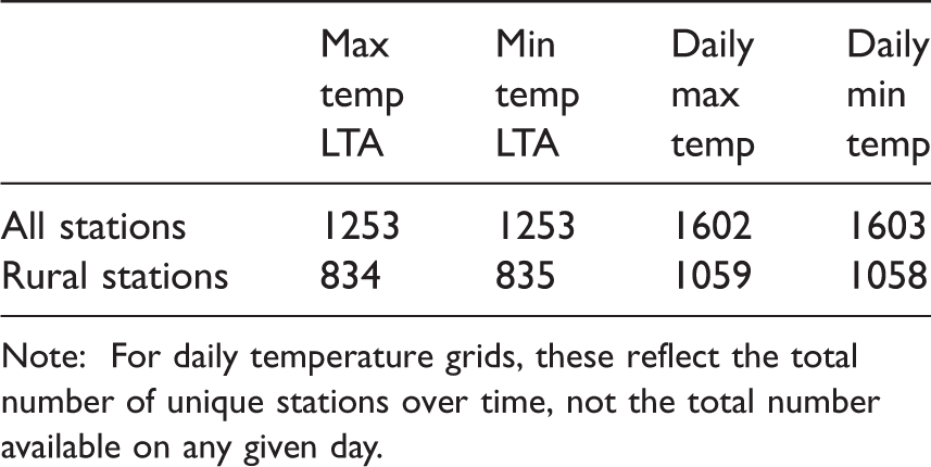
Note: For daily temperature grids, these reflect the total number of unique stations over time, not the total number available on any given day.

The interpolation scheme of PH05a,¹⁴ outlined previously, was used for evaluating the performance of the method. For evaluation, an estimate of the 1981–2010 LTA at each specific station location was made, using all other available stations within the ‘rural station’ set and the PH05a¹⁴ interpolation method, but excluding the station itself. This approach therefore gives us an interpolated estimate of a rural only LTA to compare against all stations.

Figure 3 shows the difference between the station climatology and the one estimated by the PH05a¹⁴ method excluding urban stations. The results are provided for daily minimum temperature (Tmin) during summer, which has the largest average urban heat island effect.⁸ The x-axis shows the stations urban coverage based on the 5 km AU, and data points are colour coded on the basis of whether the station is in the rural or urban set. The urban set is also separated into those sites failing both AU criteria and those failing only one. Figure 3 demonstrates that the rural only interpolation consistently under-predicts the temperature at urbanised stations, demonstrating the urban heat island influence on climatological Tmin. Figure 3 highlights the importance of considering both the immediate land use (1 km radius) as well as the surrounding area (5 km radius) as the highest UHII occurs when the urban fraction of both of these is taken into account, with the most urbanised sites in the network exceeding the rural-reference estimate by over 2°C in summer. The bias observed in Figure 3 indicates that a threshold approach based on the percentage of AU surrounding a station provides an effective index in defining whether a station displays rural or urban exposure characteristics.

Figure 3.

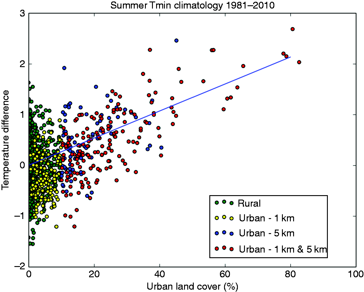
Temperature difference for a summer Tmin climatology (1981–2010) comparing station observations to an estimated climatology derived from ‘rural only’ (green) sites. The yellow, blue and red points separate locations as to whether they have an aggregated urban (AU) coverage exceeding 20% in 1 km (yellow), 10% in 5 km (blue) or both thresholds (red). The blue line is a linear fit to all points with a slope of 0.0267 and R² of 0.26.

The root mean square error from the gridding process using all available stations is 0.46°C for summer Tmin and 0.41°C for summer Tmax, consistent with Ph05a¹⁴ and summarised in Table 2. The values are actually slightly lower for the urban stations (middle row) than rural (bottom row) as the majority of the urban sites are located in well-populated areas of the country with good station coverage, whereas the rural set also includes more remote observing sites in upland areas and islands. The rural-only RMSE is determined relative to the linear trend as presented in Figure 3. The restriction to the rural-only set of stations does not degrade the overall quality of the interpolation for rural stations (bottom row) for either Tmax or Tmin. However, modest increases in the RMSE are found for urban stations in the rural-only Tmin. This is to be expected given the data exclusions. The results provide evidence that the approach is justifiable for quantifying and mapping UK urban heat islands, and uncertainty in the grid estimates will be of comparable magnitude to those in the existing PH05a¹⁴ datasets.

Table 2.

Root mean square difference (°C) between the interpolated estimated climatology and the station observation for a summer (JJA) climatology.

	Tmin (all)	Tmin (rural-only)	Tmax (all)	Tmax (rural-only)
All stations	0.46	0.50	0.41	0.42
Urban stations	0.45	0.53	0.37	0.39
Rural stations	0.47	0.47	0.43	0.43

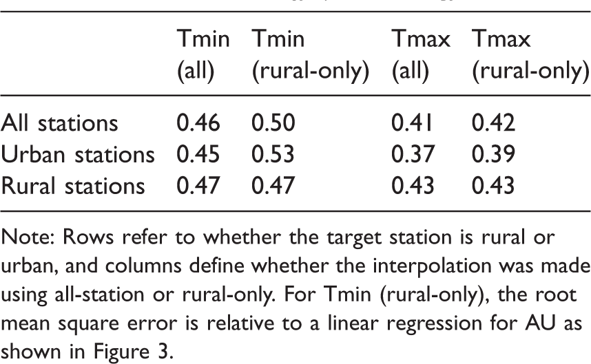
Note: Rows refer to whether the target station is rural or urban, and columns define whether the interpolation was made using all-station or rural-only. For Tmin (rural-only), the root mean square error is relative to a linear regression for AU as shown in Figure 3.

Figure 3 also shows little evidence of significant urban bias within the set of stations characterised with high AU at 1 km (yellow points). The decision to exclude these sites from the rural-set may be worth revisiting in a future iteration of this approach. In this version, they have been excluded.

Long-term climatological averages

Figure 4 shows the average difference in minimum temperature between the ‘all station’ and ‘rural only’ grids for winter (December, January and February) and summer (June July and August) 1981–2010 reference climatology. Hereafter we will refer to the temperature difference between the ‘all station’ and ‘rural only’ values as the estimated average urban heat island intensity (UHII). The maps show that the urban heat islands are most pronounced in summer minimum temperatures with prominent urban heat islands associated with the UK’s major cities including London, Birmingham, Manchester, Leeds and Liverpool. Maximum temperatures (not shown) have much weaker UHII consistent with the findings of others.^3,8,19 Uncertainty from the interpolation process described above has introduced some localised features that are not the consequence of urban heat island effects, such as negative differences directly to the south of London and in the Cardiff bay area. Some of these will be discussed in more detail below. However, for the vast majority of the country, the all-station and ‘rural only’ grids are in close agreement reflecting that even in the 21st Century a rural land surface still dominates the climatological map of the UK and the climate map derived from the reduced rural-only network is not adversely impacted by the reduced sampling. The UK mean Tmin estimated from the ‘rural-only’ network is 0.05°C lower than from the ‘all-station’ network.

Figure 4.

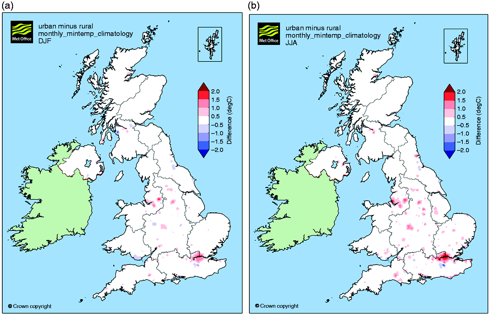
Maps showing long-term average difference between the temperature of the ‘all station’ grids compared to the temperature of the ‘rural only’ grids for daily minimum temperature in winter (a) (DJF) and daily minimum temperature in summer (b) (JJA).

Figure 5 shows the climatology of the UHII for each month estimated for a number of UK metropolitan areas for Tmin. In this plot, the average minimum temperature was determined for the areas contained within the polygons shown in Figure 2. These metropolitan areas are in many cases larger than the main urban centres, and therefore also contain non-urban areas, but they provide a useful scale at which to evaluate the regional impact of urban heat islands. The regions differ in size and levels of urbanisation so are not directly comparable to each other but the annual average values for each of the regions are shown in Table 3. Greater London is unsurprisingly the region with the largest UHII with an average of 1.1°C. The UHII climatology for daily minimum temperature is significantly larger than that of maximum temperature. Figure 5 also shows a strong seasonal cycle in the Tmin UHII, peaking in July. This is not present in the Tmax UHII (not shown).

Figure 5.

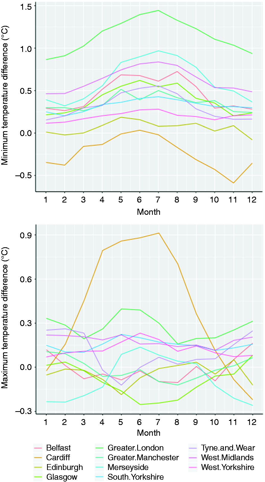
Monthly estimated 1981–2010 average UHII for (top) daily minimum temperature, and (bottom) daily maximum temperature for UK metropolitan areas.

Table 3.

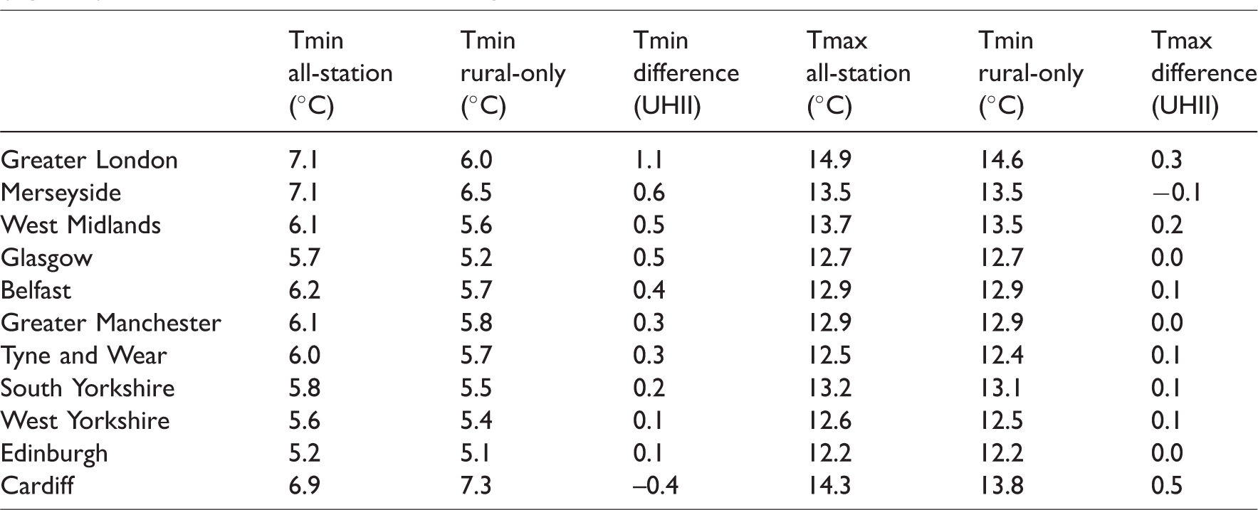
1981–2010 climatological annual mean temperatures for Tmin and Tmax averaged over metropolitan areas (Figure 2) from the ‘all-station’ and ‘rural-only’ networks.

	Tmin all-station (°C)	Tmin rural-only (°C)	Tmin difference (UHII)	Tmax all-station (°C)	Tmin rural-only (°C)	Tmax difference (UHII)
Greater London	7.1	6.0	1.1	14.9	14.6	0.3
Merseyside	7.1	6.5	0.6	13.5	13.5	−0.1
West Midlands	6.1	5.6	0.5	13.7	13.5	0.2
Glasgow	5.7	5.2	0.5	12.7	12.7	0.0
Belfast	6.2	5.7	0.4	12.9	12.9	0.1
Greater Manchester	6.1	5.8	0.3	12.9	12.9	0.0
Tyne and Wear	6.0	5.7	0.3	12.5	12.4	0.1
South Yorkshire	5.8	5.5	0.2	13.2	13.1	0.1
West Yorkshire	5.6	5.4	0.1	12.6	12.5	0.1
Edinburgh	5.2	5.1	0.1	12.2	12.2	0.0
Cardiff	6.9	7.3	–0.4	14.3	13.8	0.5

Cardiff is displaying unusual behaviour with a negative UHII for minimum temperature and larger positive value for maximum. Cardiff is an example of an urban centre for which this particular methodology has proven to be ineffective. Figure 2 shows that all the near coastal sites in this part of south Wales are in the ‘urban’ set of stations. The rural sites that will be driving the interpolation for Cardiff are at Flat Holm, a small island 6 km off the coast, and Cilfynydd at an elevation of 194 m. The interpolation process is failing to adequately reproduce the climate of the low-lying area around Cardiff and surroundings from these rural sites located in rather different local climate regimes. This could help inform future network design for a suitable rural reference site for climate in this part of south Wales. In contrast in other parts of the country, the exclusion of urban stations can create relatively larger gaps in the network, but with less marked topographic and climatological differences, the urban signal still dominates. The general expected uncertainty is also reflected in Figure 3 and Table 2.

Long-term trends in UHII

In this and subsequent sections, analysis is based on the gridding of daily temperature values following PH09¹⁵ rather than long-term averages. These are used to investigate trends and variability in UHII. Figure 6 shows time series of the annual average difference between the ‘rural only’ and ‘all stations’ grids daily minimum temperature over each metropolitan area. There is no consistent picture of increasing or decreasing UHII across these UK metropolitan areas. However, there are some notable exceptions, such as a decline in UHII for the West Midlands region, and large step changes in the Cardiff series. At regional/local scales, the interpolation process presented above can be sensitive to the availability of particular stations. These inhomogeneities in the Cardiff series coincide with the opening and closing of Cardiff weather centre (opening in 1980 and closing in 2006).

Figure 6.

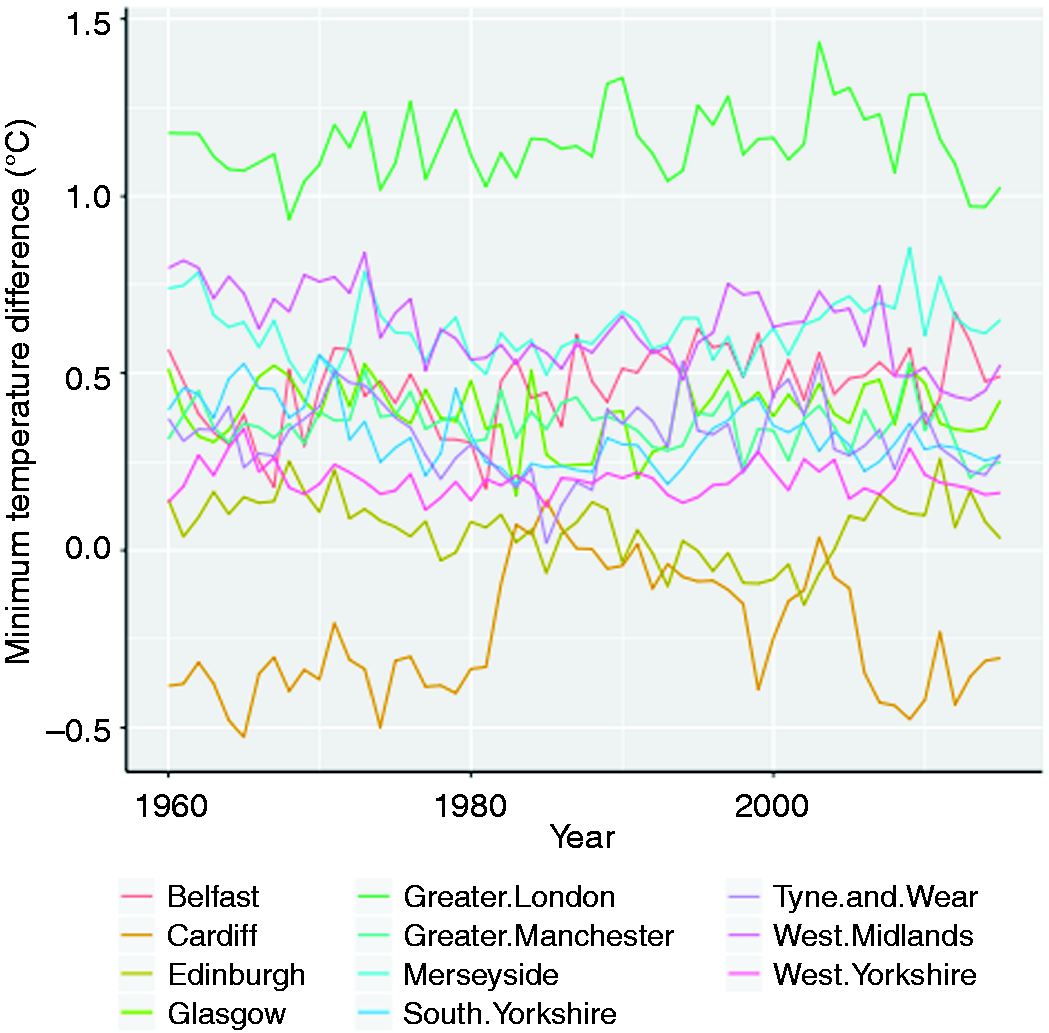
Time series of estimated annual average Tmin UHII for metropolitan areas derived from the difference between the ‘all stations’ and ‘rural only’ grids.

The change at Cardiff is particularly dramatic, but other decadal trends in UHII are apparent in Figure 6. Long-term variability in UHII has been documented elsewhere (for example Wilby et al.³); however, we cannot rule out that non-climatic factors in the underlying observing network contribute to variations shown in Figure 6. We therefore conclude that the methodology presented here is, at the time of writing, unsuitable for the analysis of long-term trends or decadal scale variability in city-scale urban heat islands.

However, as stated previously, the removal of urban sites from the ‘rural-only’ network has a modest impact on UK mean temperature of the order 0.05°C. This provides further support that the PH05a,¹⁴ PH05b¹³ and PH09¹⁵ methods are robust to changes in the underlying network at the national scale, and that furthermore urbanisation in the UK is unlikely to have had a major influence on the observed UK-scale warming during the 20th century as presented in Kendon et al.²⁰

Daily variability

The areal average minimum temperature and maximum temperature for the metropolitan areas were produced for each day to produce an estimate of the UHII influence at a daily scale over the period 1960–2015. The analysis examined whether the variance in the difference differed over the distribution of temperatures (i.e. exhibited heteroscedasticity). These area average statistics will not reflect the peak in UHII that will usually be located close to the geographical city centre; however, the area averaging does reduce the spatially random component of both observational and interpolation uncertainty. In this and subsequent analysis, we present the results for Greater London which has the largest UHII signal.

Figure 7 shows the time series of the UHII over the Greater London region. The corresponding histograms show the distribution of daily UHII estimates. The UHII for minimum and maximum temperature have mean of 1.1°C and 0.3°C (see also Table 3) and standard deviation of 0.7°C and 0.4°C, respectively. The minimum and maximum UHII have skewness of 0.6 and 0.08 and kurtosis of 3.1 and 5.3, respectively. The greatest difference (irrespective of sign) in the UHII time series over the Greater London region was larger for Tmin compared to the Tmax (4.3°C vs. 3.2°C). This is consistent with a greater influence of urban heat islands at night.

Figure 7.

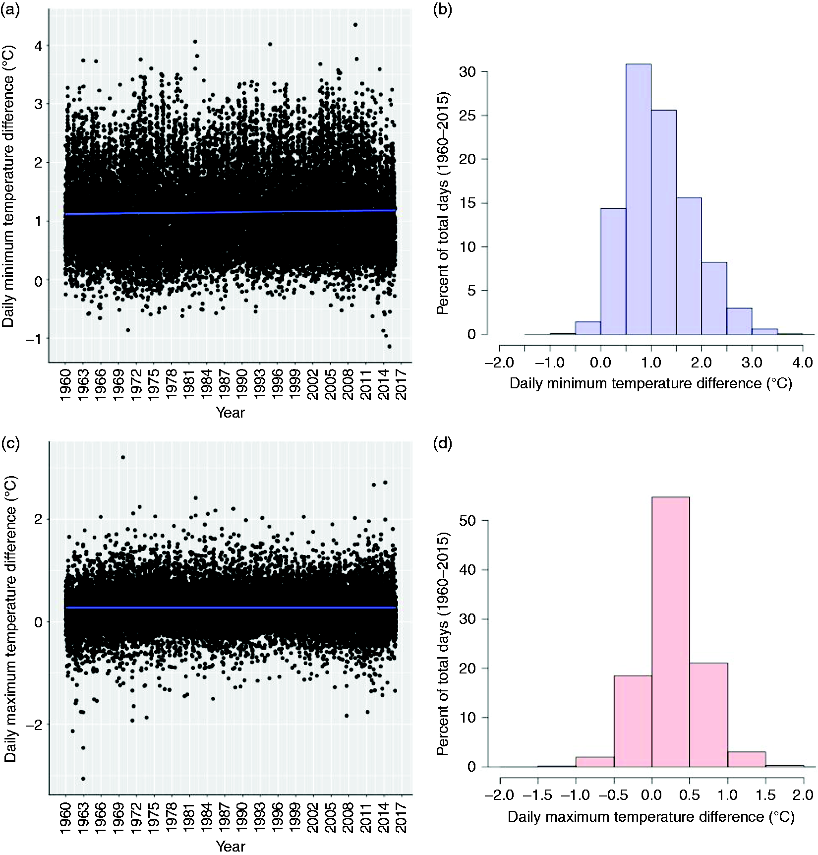
(a) Time series of the daily Tmin UHII estimated over the Greater London region. (b) Histogram showing the distribution of these daily differences. (c) + d) as (a) and (b) but for Tmax.

Figure 8 shows the differences between daily minimum and maximum UHII over the Greater London region plotted against the coincident ‘rural only’ grid temperatures. These show little heteroscedasticity except at the lowest temperatures where UHII increases, i.e. the UHII is most likely to be large during the coldest nights. Although the average UHII intensity is largest during the summer months (as shown in Figure 4), the coldest winter nights also exhibit a strong UHII, but temperatures below −10°C are relatively infrequent for this part of the UK.

Figure 8.

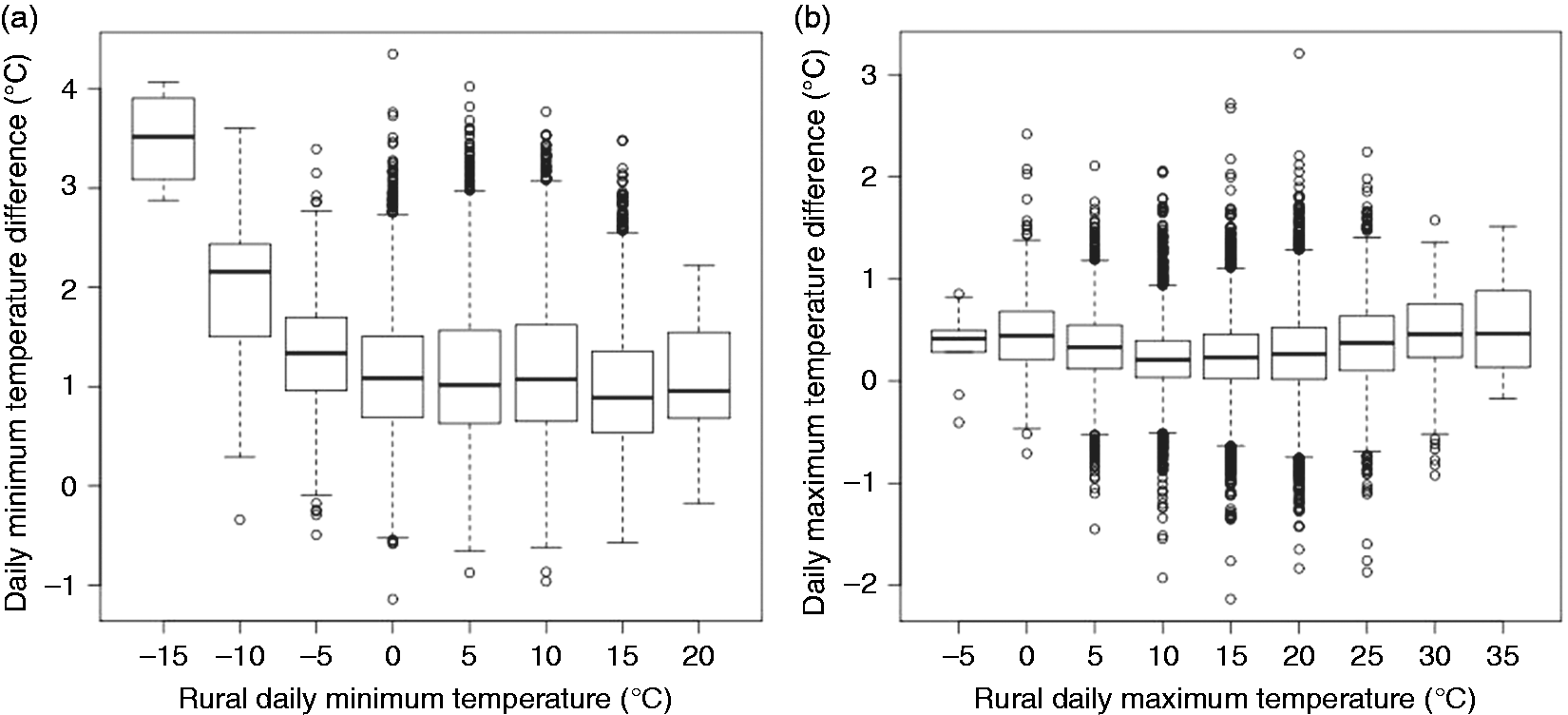
Estimated average UHI over the Greater London region based on the temperature difference between the ‘all station’ and ‘rural only’ grids (see text) against the ‘rural only’ grid temp mean temperature (x-axis) for (a) daily minimum and (b) daily maximum temperature.

Figure 9 shows the daily minimum temperature UHII against the daily maximum temperature from the previous day. Urban areas have a much higher heat capacity as well as a lower solar reflectance than rural materials giving rise to strong radiative heating of the urban infrastructure under sunny and hot conditions. These processes result in the formation of substantial night-time urban heat islands. There is also some evidence in Figure 9 of higher than average nocturnal UHII under the coldest conditions when day time maximum temperatures are at or below freezing. It is speculated that increased anthropogenic heat flux from central heating of buildings combined with generally low wind speeds and minimal mixing under such cold conditions could be a significant contributing factor to the UHI in these circumstances.

Figure 9.

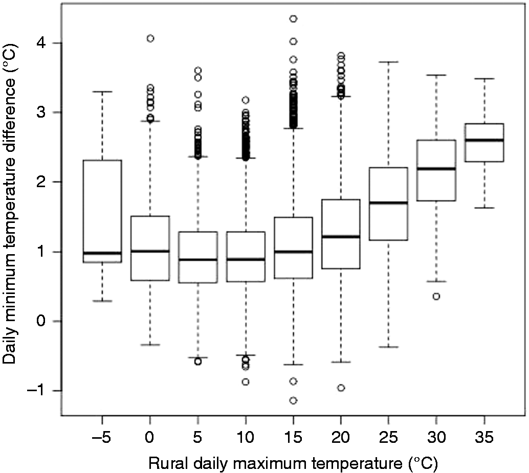
Estimated distribution of daily minimum UHII over the Greater London region against the maximum temperature from the preceding day.

Meteorological effects that explain fluctuations in these daily differences such as cloud cover and wind were examined. The Met Office do not generate comparable gridded datasets of daily cloud cover and wind observations, therefore hourly observations taken at Heathrow were chosen to be representative of the Greater London region. The meteorological data were split into night time and daytime values to differentiate the normal time of day when the daily minimum and maximum temperature occur. Daytime values were defined as the mean of the hourly observation between 6 a.m. and 6 p.m. and night time was calculated as the mean between 6 pm and 6 a.m.

Figure 10 shows the observed cloud cover during night and day against the daily estimated UHII for minimum and maximum temperatures. Larger positive UHII occurs when under clear skies. This is more significant for minimum temperature than maximum temperature and larger impact in summer than winter.

Figure 10.

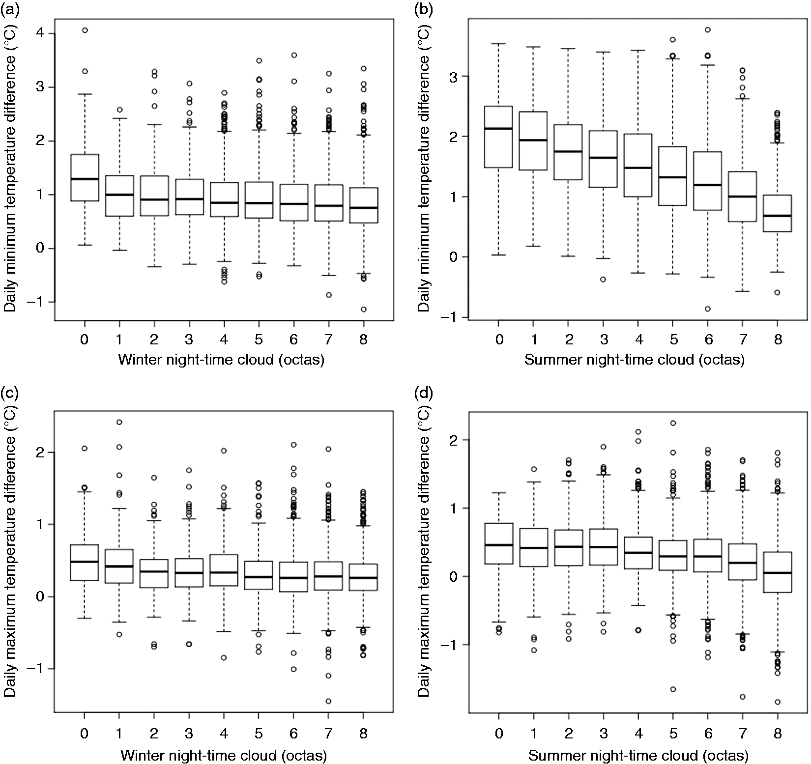
Average cloud cover at nightime recorded at Heathrow against the estimated daily minimum temperature UHII over the Greater London region (a) during the winter, (b) during the summer. Average cloud cover during day time against estimated daily maximum temperature UHII over the Greater London region (c) during the winter (d) during the summer.

Figure 11 shows the night time and day time wind speed against the daily UHII in minimum and maximum temperature. Larger UHII occurs on the days when wind speeds were low. The relationship is stronger for daily minimum temperature than maximum temperature and stronger in summer than winter for minimum temperature, but for maximum temperature there is greater influence of wind speed on the winter UHII. This follows the expected scenario for urban heat islands to develop in low wind speeds when lateral advection is supressed. The signal is not as strong with the daily maximum temperature, as expected from urban heat island effects having less effect on higher temperatures, when vertical mixing is stronger and the surface boundary layer is deeper. Nevertheless, the variance increases with light winds in winter with additional contribution from anthropogenic heating. In summer, any effect on the maximum temperature difference due to wind speed is insignificant as the near surface air is more readily mixed vertically even with weak horizontal winds.

Figure 11.

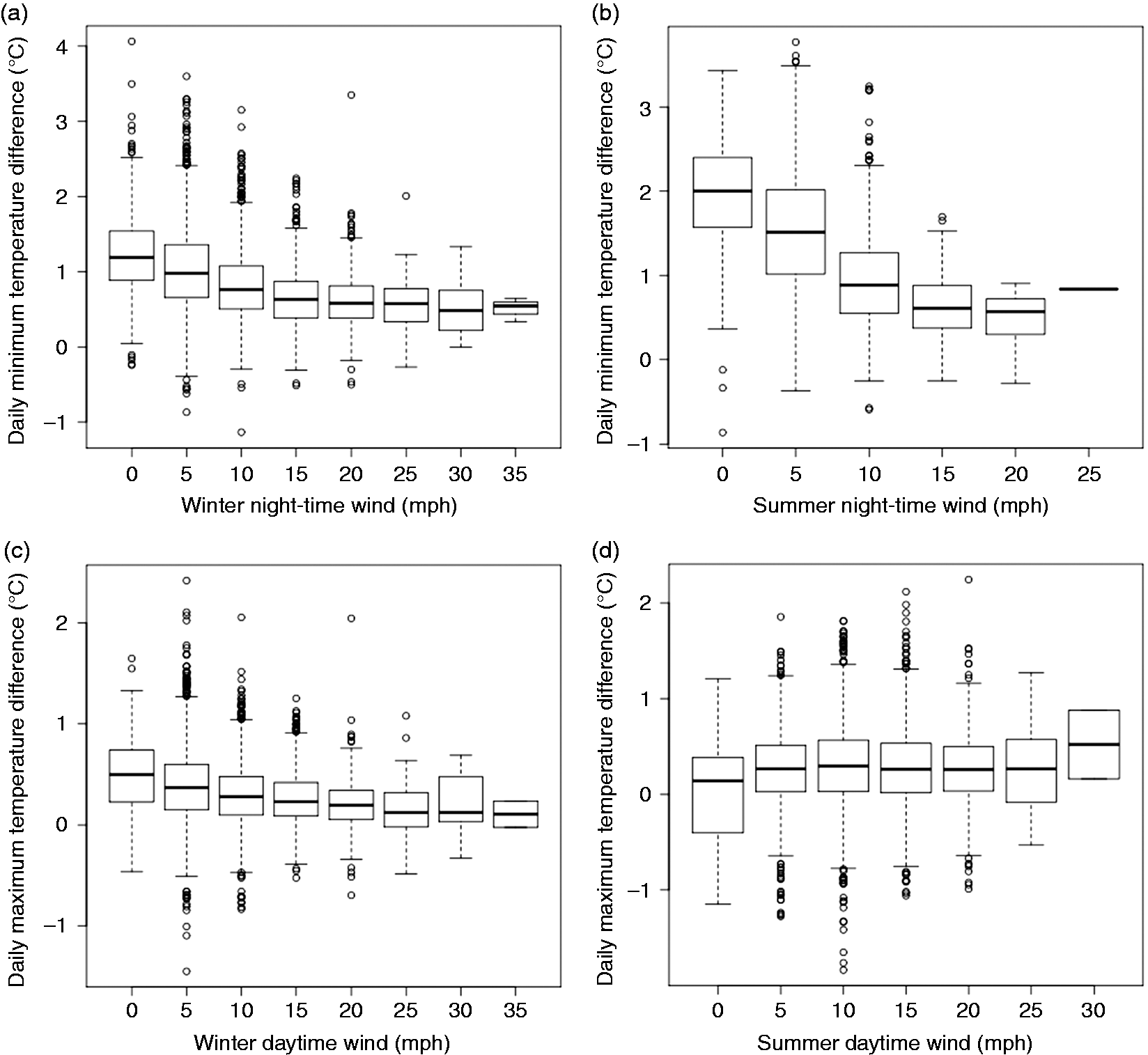
Average wind speed during the night time (mph) recorded at Heathrow against the estimated daily minimum temperature UHII over the Greater London region (a) during the winter (b) during the summer. Average wind speed during the day time (mph) recorded at Heathrow against the estimated mean daily maximum temperature UHII over the Greater London region (c) during the winter (d) during the summer.

In the previous section, we demonstrated that long-term trends and variability in the dataset were compromised by non-climatic inhomogeneities. In this section, we have demonstrated that the daily-scale analysis of UHII has some climatological value for exploring the variability of UHII for major cities in the UK. Individual locations and days will be subject to uncertainty in the estimated temperature of order 1°C.¹⁵ However, with such a large sample of daily data, we have demonstrated that the method is able to describe the expected climatological characteristics of urban heat islands. Thus, the daily analysis has value as a climatological tool to explore characteristics of UHII under a range of UK meteorological conditions from a sample of 55 years of daily data.

Spatial detail

The previous sections have explored city to regional scale of metropolitan areas. Next we evaluate the representivity of individual grid point values at the 5 km scale of the dataset. Figure 12 compares the mean UHII for Greater London region (x-axis) with the highest UHII at any grid point within the region (y-axis) for all days in the period 1960–2015. Based on a linear regression of the data in Figure 12, the peak UHII (which will generally be located close to the centre of the city) for Greater London is approximately double the size of the estimated mean UHII with a spread of approximately 1°C. For example, an average UHII for Greater London of 2°C might be associated with a peak UHII of at least 4°C ± 1°C.

Figure 12.

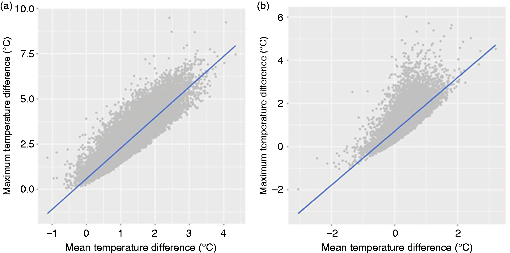
(a) Difference between the estimated mean daily minimum temperature UHII over the Greater London region and maximum UHII within the region (y = 1.7x + 0.6) (b) As (a) for daily maximum temperature UHII (y = 1.2x + 0.7).

The pattern of behaviour of temperature across cities for individual days will be influenced by a multitude of meteorological factors. In one particularly large discrepancy on 1 November 2015, the Greater London estimate of UHII by this method was −1.3°C (a negative or cool island), with a peak grid point UHII of 2.5°C. However, weather observations on 1 November 2015 recorded patchy fog resulting in particularly large localised variations in temperature. This caused the large discrepancy between the point values and areal average. The fog can also account for the negative difference between the ‘rural only’ and ‘all station’ grids as the fog in London meant that several observation sites in the all station grids over the London area were colder than the surrounding rural sites. The interpolation scheme used in this method does not have any knowledge of other meteorological factors, such as fog, therefore the differences at individual locations and days in the dataset will also contain influences from these. Application of this dataset should, as already stressed above, focus on the statistics of the large sample of days rather than the details of any specific day, for which additional meteorological data may be required for context.

Hot spells and cold waves

The statistics of heat and cold has also been analysed. A threshold approach will be used to define the heat wave and cold waves as such it is to be expected that the length and frequency of heat and cold waves will be altered by the presence of the urban heat islands – more and longer heat waves, fewer and shorter cold waves. This has been tested for the Greater London region by examining sequences of maximum temperature above 25°C and minimum temperatures below −5°C

The number of consecutive days when the daily maximum temperature exceeded 25°C over Greater London was calculated from the time series of mean daily maximum temperature derived from the ‘all stations’ and ‘rural only’ grids. A histogram of the duration of these events using the two grids can be seen in Figure 13. Beyond a five-day duration, the two distributions are comparable suggesting that urban heat islands do not extend the duration of longer heatwave events, for which the driver is the large scale synoptic conditions. However, there is an increase in the frequency of the two to four day events.

Figure 13.

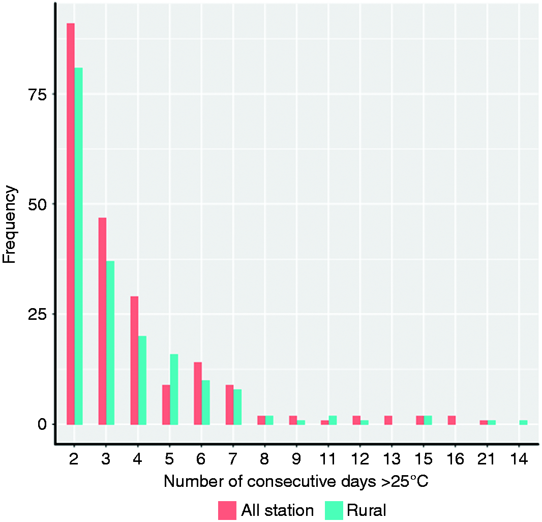
Histogram showing the distribution of number of consecutive days on which the daily maximum temperature exceeded 25°C over Greater London derived using the ‘rural only’ maximum temperature grid (blue fill) compared to that derived from the all station grid (red fill).

The longest duration of consecutive daily maximum temperatures exceeding 25°C was recorded during the heatwave of 1976. Figure 14 shows the daily maximum temperature over Greater London during this period derived using both the ‘all stations’ and the ‘rural only’ daily maximum temperature grids. The datasets suggest that the urban heat island does increase the peak temperatures recorded on the hottest day of the heatwave (26th June) by 0.7°C, with a maximum of 34.1°C in the all-station grid compared to 33.4°C in the rural-only (the highest value at any individual grid cell was 34.8°C in the all-station grid and 34.1°C in the rural only, the highest station values in London were 34.8°C at Heathrow and London Weather Centre). However, the UHII has no effect on the event duration, that is dictated by the larger-scale variability. This is consistent with the findings of others, that the urban heat island effect is larger in the daily minimum temperature values than the maximum temperature.^3,8,19

Figure 14.

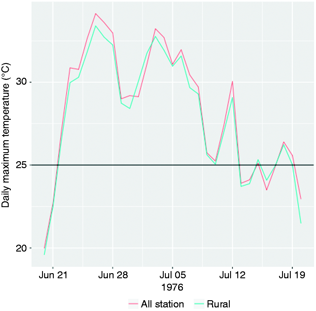
Daily maximum temperature over Greater London in July 1976 derived using the ‘all stations’ daily maximum temperature grid (red line) and ‘rural only’ grid (blue line).

The distribution in UHII for daily maximum and minimum temperature in Greater London during heatwave events has been plotted in Figure 15. The histogram shows that the UHII in daily maximum temperature is relatively small with a mean of 0.5 ± 0.4°C, whereas the daily minimum temperature UHII is 2.0 ± 0.7°C. The UHII estimate for daily minimum temperature averaged across Greater London for all days between 1960 and 2015 is 1.1 ± 0.7°C. The increase in the average minimum temperature difference from 1.1 ± 0.7°C to 2.0 ± 0.7°C during heat waves suggests that the effects of urban heat islands on daily minimum temperature are on average more substantial during heatwaves. The elevated night temperatures are important for public health, and also for the performance of buildings in cities with reduced capacity to lose the heat built up during the daytime.

Figure 15.

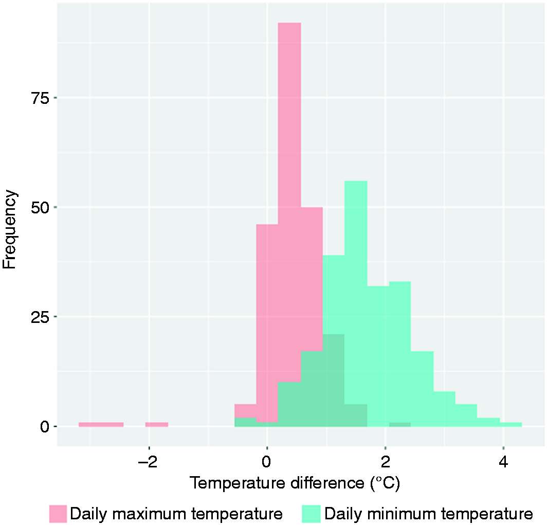
Histogram showing the distribution of estimated UHII over Greater London during events when the daily maximum temperature exceeded 25°C. The red histogram represents UHII in the daily maximum temperature and blue histogram represents UHII in the daily minimum temperature (purple represents areas where the distributions overlap).

The number of consecutive days when the daily minimum temperature fell below −5°C over Greater London has been calculated in the same way. The distribution of these events has been plotted in Figure 16. The figure shows that the urban heat island significantly reduces the number and duration of ‘cold wave’ events for the city.

Figure 16.

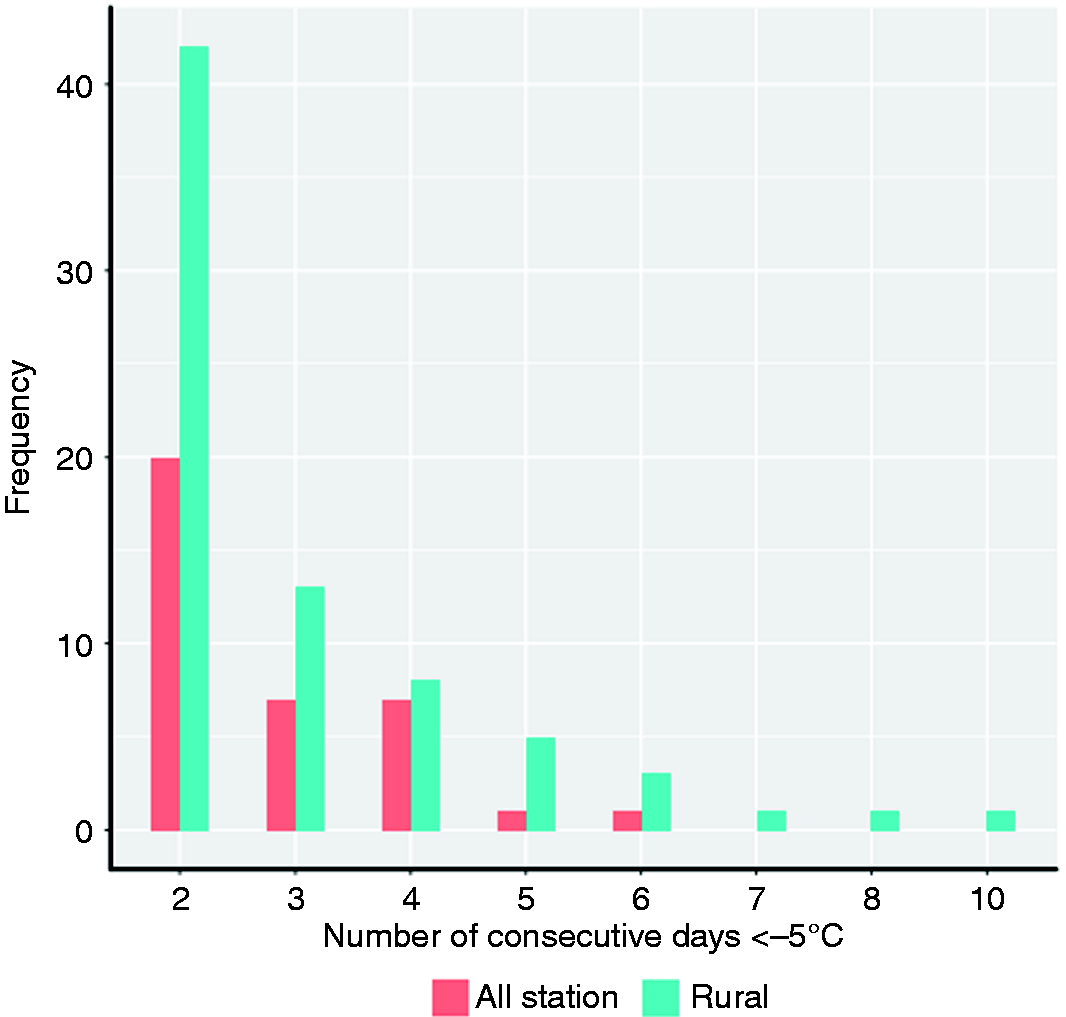
Histogram showing the distribution of number of consecutive days on which the daily minimum temperature fell below −5°C over Greater London derived using the ‘rural only’ (blue fill) minimum temperature grid compared to that derived from the ‘all stations’ grid (red fill).

The longest number of consecutive days with a minimum temperature below −5°C for Greater London occurred in January 1963. Figure 17 shows the daily minimum temperature for January 1963 averaged over Greater London derived using the ‘all stations’ and ‘rural only’ grids. The graph shows that the ‘rural only’ grid is consistently colder than the ‘all stations’ grid. On the coldest day (23 January), the rural-only grid for Greater London saw temperatures falling below −15°C with a sequence of five days below −10°C. In the all-station grid, the UHII reduced the severity with a minimum temperature of −11.9°C on the 23rd, and a sequence of three days below −10°C. As stated in previous sections, the quantification of individual days needs to be treated with some caution due to the uncertainties. However, in this case, the evidence supports that the presence of London’s UHII significantly reduced the severity of the January 1963 cold spell for the urban population.

Figure 17.

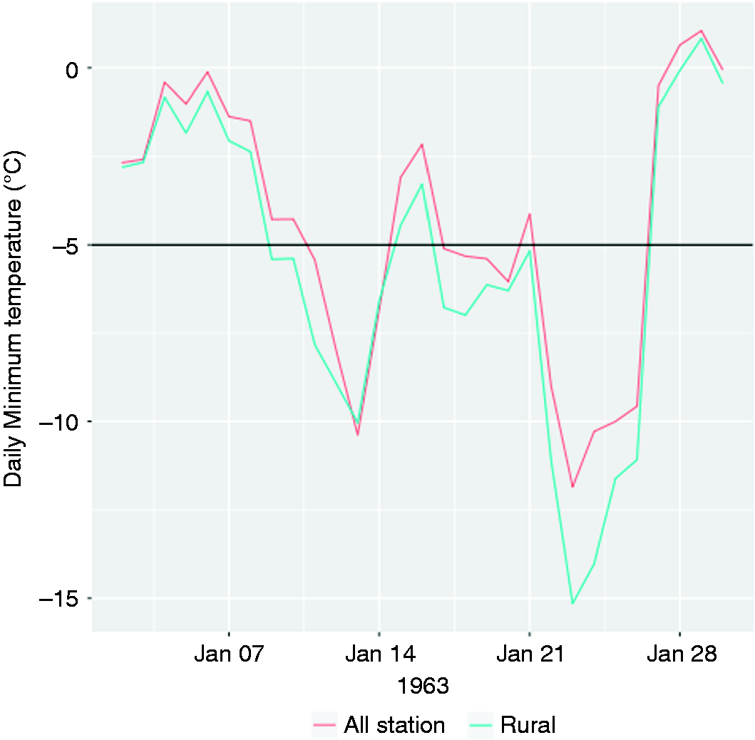
Daily minimum temperature over Greater London in January 1963 derived using the ‘all stations’ daily minimum temperature grid (red line) and ‘rural only’ grid (black line) compared to the threshold of −5°C (black horizontal line)).

Discussion and conclusions

UK gridded datasets of the differences in long-term climatology in both the maximum and minimum temperature across the UK have been generated from a ‘rural only’ and ‘all stations’ network. The largest differences in the temperature between the two grids occur over urban areas as a consequence of the urban heat island. The results found here are consistent with, but expand on existing studies of UK urban heat islands, by providing a climatological reference set for UK cities with a sample of 55 years of daily observationally based analyses.

Analysis of the daily differences in the temperature of the ‘rural only’ and ‘all stations’ grids across 11 metropolitan areas demonstrates that positive differences in the temperature data between the ‘all stations’ and ‘rural only’ grid could in most cases be attributed to urban heat island effects. When comparing maximum and minimum temperatures, the differences are largest between the ‘rural only’ and ‘all stations’ grid daily for minimum temperatures, with a mean difference ± SD over Greater London of 1.1 ± 0.7°C compared with 0.3 ± 0.4°C for maximum temperatures. For most metropolitan areas, the average difference between the minimum temperature between the ‘all stations’ and ‘rural only’ grids is largest in summer. This seasonal variation is driven by a positive correlation between the difference in the daily minimum temperature derived from the ‘all stations’ grid and ‘rural only’ grid not present for the daily maximum temperature. This is consistent with the difference in the heat capacity and reflectivity of urban surfaces compared to that of rural materials resulting in heat islands tending to develop at night time after hot sunny days.

The difference between the “all station “and “rural only” minimum temperature grids averaged over Greater London in summer was 1.4 ± 0.7°C and the maximum UHI recorded within Greater London over the same period was 2.8 ± 1.4°C (in agreement with Watkins et al.⁵). Figure 12 shows that although the average UHI measured across the London metropolitan area does not exceed 4°C, localised extremes can be seen exceeding 8°C in agreement with previous estimates by Watkins et al.⁵ that the summer heat island intensity in London reaches a maximum of 8°C but for only a small proportion (1%) of the time.

Although the overall difference between the ‘all stations’ grid and ‘rural only’ grid minimum temperature is smaller in winter, the magnitude of individual events in the winter can be as large as that observed in the summer. There is also a negative correlation between the magnitude of the heat island and the rural daily minimum temperature at very cold temperatures (below −5°C). This may be because the type of pressure pattern that normally causes these very low temperatures in the winter also result in other meteorological factors that are conducive to the development of heat islands.

It was possible to relate daily fluctuations in the differences during the summer and winter to other meteorological factors such as wind and cloud cover. The difference between the grids over Greater London reduces with wind speed consistent with urban heat islands being more likely to occur on days with low wind speeds. The difference also increases with decreasing cloud cover. A decrease in cloud cover is closely correlated to an increase in the daily sunshine amounts, therefore these findings are consistent with the processes that result in the formation of urban heat islands. The relationship between these meteorological parameters and the formation of a UHI is strongest in the summer and at night time. For example, on summer days with high radiation, i.e. low cloud cover days (classified as below 1 octa), the “all stations” – “rural” contrast in minimum temperature over the Greater London region is 2.2 ± 0.7°C with localised maximum differences of 4.2 ± 1.2°C, the latter magnitude is in line with expected magnitudes on days conducive to the formation of the UHI.⁶

Urban heat islands have a much larger effect on minimum temperature than maximum temperature. As a consequence, the distribution of hot spell events over Greater London (defined as an event when the daily maximum temperature exceeded 25°C for two or more consecutive days) does not change that significantly when using the ‘rural only’ or ‘all stations’ grid. However, the daily minimum temperature of Greater London during these events was consistently higher when it was calculated from the ‘all stations’ grid compared to the ‘rural only’ grid with an average temperature difference of 2.0 ± 0.7°C. The distribution of consecutive days in which the minimum temperature fell below −5°C (cold waves) changed significantly as both the frequency and the duration of the events decreased when the events were calculated from the daily minimum temperatures derived from the ‘all stations’ grid rather than the ‘rural only’ grid.

Whilst there is considerable potential utility for this dataset, there are a number of limitations that have been identified in this analysis. Firstly, observation stations are typically located in rural areas or slightly outside the centre of a city (Figure 2). This means that some stations classified as rural may be influenced by urban areas, especially if a station is downwind of a city centre.²¹ Urban stations can also be influenced by micro climates e.g. parks, as demonstrated in Figure 1.3 and 1.4, respectively. These types of confounders may result in an underestimation of the UHII in this analysis.

Secondly, land use is assumed to be fixed throughout the gridding period (1960–2015) using The Centre for Ecology and Hydrology land cover map 2007 to classify the urban land exposure for the UK observing network. However, there is no consistent picture of increasing or decreasing UHII across the UK metropolitan areas suggesting that change in land use due to urbanisation has not had a large influence on temperature biases within the observing network.

Some small scale features at resolutions close to that of the 5 km scale of the grids and variations from day to day have been identified in this project that may not originate from urbanisation impacts. These will include, but not be limited to, small scale features such as localised fog and more generally uncertainty introduced from the statistical interpolation algorithms used, for which the uncertainties are documented in PH05a,¹⁴ PH05b,¹³ and PH09.¹⁵

The method has been demonstrated to be ineffectual for some smaller cities within areas of complex terrain, such as Cardiff in south Wales where rural reference stations are located on islands or at higher elevation. The trends for individual cities can also be prone to inhomogeneities arising from changes in the underlying observing network, and therefore the dataset in its current form is not suitable for the study of inter-annual trends in UHII. Further work would need to be carried out to understand the sensitivity of the bias and variance within the bias to the station network density in both ‘rural only’ and ‘all stations’ grids.

However, the utility of this unique daily climatology of urban climates of the UK has value for exploring some of the statistical properties and behaviour through a very large sample of weather conditions.

Footnotes

Declaration of conflicting interests

The author(s) declared no potential conflicts of interest with respect to the research, authorship, and/or publication of this article.

Funding

The author(s) disclosed receipt of the following financial support for the research, authorship, and/or publication of this article: This work was supported by EPSRC grant EP/M021890/1.

ORCID iD

K Chowienczyk

References

Howard

Climate of London deduced from meteorological observation.

Harvey Darton1833; 1: 1–24.

Arnfield

AJ.

Two decades of urban climate research: a review of turbulence, exchanges of energy and water, and the urban heat island.

Int J Climatol 2003; 23: 1–26.

Wilby

Jones

Lister

DH.

Decadal variations in the nocturnal heat island of London.

Weather 2011; 66: 59–64.

Tomlinson

Chapman

Thornes

, et al. Derivation of Birmingham's summer surface urban heat island from MODIS satellite images. Int J Climatol 2012; 32: 214–224.

Watkins

Palmer

Kolokotroni

, et al. The London heat island: results from summertime monitoring. Build Serv Eng Res Technol 2002; 23: 97–106.

Smith

Webb

Levermore

, et al. Fine-scale spatial temperature patterns across a UK conurbation. Climatic Change 2011; 109: 269–286.

CIBSE Guide A2. The Chartered Institution of Building Services Engineers (CIBSE) guide A, environmental design. London: CIBSE, 2015.

McCarthy

Harpham

Goodess

, et al. Simulating climate change in UK cities using a regional climate model, HadRM3. Int J Climatol 2012; 32: 1875–1888.

Stewart

ID.

A systematic review and scientific critique of methodology in modern urban heat island literature.

Int J Climatol 2011; 31: 200–217.

10.

Voogt

Oke

TR.

Thermal remote sensing of urban climates.

Remote Sens Environ 2003; 86: 370–384.

11.

Best

Grimmond

CS.

Key conclusions of the first international urban land surface model comparison project.

Bull Am Meteorol Soc 2015; 96: 805–819.

12.

Kershaw

Sanderson

Coley

, et al. Estimation of the urban heat island for UK climate change projections. Build Serv Eng Res Technol 2010; 31: 251–63.

13.

Perry

Hollis

The development of a new set of long‐term climate averages for the UK.

Int J Climatol 2005; 25: 1023–1039.

14.

Perry

Hollis

The generation of monthly gridded datasets for a range of climatic variables over the UK.

Int J Climatol 2005; 25: 1041–1054.

15.

Perry

Hollis

Elms

The generation of daily gridded datasets of temperature and rainfall for the UK. National Climate Information Centre, Met Office, Exeter, www.metoffice.gov.uk/binaries/content/assets/mohippo/pdf/ukclimate/papers/cm24_generation_of_daily_gridded_datasets.pdf. (2009, accessed 23 September 2019).

16.

Met Office. Met Office Integrated Data Archive System (MIDAS) land and marine surface stations data (1853 - current), http://catalogue.ceda.ac.uk/uuid/220a65615218d5c9cc9e4785a3234bd0 (accessed 23 September 2019).

17.

Morton

Rowland

Wood

, et al. Land cover map (vector, GB) v1. 2, 2007.

18.

Oke

TR.

Initial guidance to obtain representative meteorological observations at urban sites, www.wmo.int/pages/prog/www/IMOP/publications/IOM-81/IOM-81-UrbanMetObs.pdf (accessed 23 September 2019).

19.

Zhou

Zhang

Hao

, et al. Spatiotemporal trends of urban heat island effect along the urban development intensity gradient in China. Sci Total Environ 2016; 544: 617–626.

20.

Kendon

McCarthy

Jevrejeva

, et al. State of the UK climate 2017. Int J Climatol 2018; 38: 1–35.

21.

Bohnenstengel

Evans

Clark

, et al. Simulations of the London urban heat island. Quarter J Royal Meteorol Soc 2011; 137: 1625–1640.