Comprehensive model of linear PMSM-based ropeless lift for comparing control algorithms – Field-oriented control versus direct torque control

Abstract

This is a further study of two previous articles of the authors. The simulation model includes saliency and almost all common imperfections of linear permanent magnet synchronous machine. Based on the same model, three types of control have been applied to drive the lift car for a typical fully loaded upward journey, namely field-oriented control, which was used in two previous articles, direct force control (conventional direct torque control on a linear machine) and a newly proposed direct speed control (a new direct torque control method that could be used in the lift industry). The performances in terms of speed accuracy during start-up and rated speed operation, power and energy consumption have been studied. The conclusion is that for such a new application in the lift industry, at this moment in time, the more conventional field-oriented control is highly recommended. Two new findings are reported. Direct speed control that involves a simpler circuitry and reasonable speed control is proposed, although there is always a small steady-state error due to the absence of a proportional–integral controller. Conventional direct torque (force) control involves continuous integration to estimate the magnetic fluxes, which is not applicable to a permanent magnet synchronous machine with saliency. A new definition to analytically estimate the magnetic flux linkages in real time is also proposed. It should be noted that field-oriented control is superior at this time. When technology continues to get advanced, direct force control and direct speed control may one day be more appropriate for linear permanent magnet synchronous machine application. The software to perform the simulation has been uploaded to the BSER&T/SAGE website.

Practical application: It is generally agreed by the lift industry that the installation of multi-dimensional lifts employing linear permanent magnet synchronous machines is a clear trend in the future. This article is a follow up of two previous ones, studying the performance of three types of control for linear permanent magnet synchronous machine. Necessary equations of the machine model, imperfections, digital control loops are included. Some findings regarding the differences in performance are reported. It is hoped that this article is useful for lift manufacturers to enter this new market of vertical transportation.

Keywords

Ropeless lift linear PMSM field-oriented control direct torque control direct force control direct speed control saliency modelling of imperfections

Introduction

In our previous paper of this series,¹ it was stated that as buildings are getting taller, the provision of multiple and independent lift cars within one hoistway is the obvious solution to achieve a desirable handling capacity with a reasonable waiting time, round trip time or transit time. As buildings are also getting wider, the provision of a two- to three-dimensional hoistway network is also an obvious solution. Here, the term ‘three-dimensional’ means that every lift car is allowed to travel in three independent directions, namely up–down, right–left (say along the x-axis of the building) and forward–backward (say along the y-axis of the building). The traffic analysis of such a lift system was performed.^2–4

In order to realize and implement such a concept of independent multi-car three-dimensional lift system, the use of ‘ropeless technology’ is also a suitable solution.^1,5,6 In the industry, the first full-scaled prototype of a two-dimensional lift system was developed in Germany, called MULTI™.⁷ Although the first version of MULTI™ was two-dimensional, it is possible to extend it to a true three-dimensional application. The core technology of such a system lies with the employment of linear permanent magnet synchronous machines (LPMSMs). A simplified ideal mathematical model without the consideration of various imperfections and external forces was used to illustrate how such a LPMSM could move a ropeless lift¹ in terms of jerk, acceleration, deceleration and rated speed operation. Moreover, the most important illustration was the emergency operation when all stator windings along the walls of the hoistways were short-circuited so that the lift car could descend slowly, i.e. at the maintenance speed or even lower, to the ground floor for releasing the trapped passengers under a genuine electric power failure. The exact descending speed could be estimated analytically.

Then, imperfections of such LPMSM were considered,⁸ including the existence of reluctance force due to the difference in inductance along the d- and q-axes because of the existence of saliency. Variation in the pole pitch and external forces such as friction and end effect, etc. were also investigated. The existence of imperfections complicated both the simulation and control models and as a result, one more controller, in addition to the existing two in the simplified model, had to be added. That associated control was based on the traditional field-oriented control (FOC) method. As expected, the analytical estimation of the free falling speed under emergency operation by short-circuiting all stator windings became more complicated. But it could still be calculated by a quartic equation (fourth-order polynomial equation). And the mathematics made it possible to find out the appropriate motor parameters to achieve a falling speed of 0.2 m/s or lower. In order not to increase the complexity of the model too much, damper windings that represented the existence of an aluminium plate to cover the permanent magnets at the rotor were ignored in the last article though the mathematical model was presented.

In this article, we consider the simulation of the full model with the inclusion of the damper windings. In other words, damper windings are considered and included in all simulation loops but not in the control loops in order to simplify the control equations. By doing so, the results are still considered satisfactory. Furthermore, regarding control methods, FOC, the classic variable speed vector control for AC machines used in our previous papers,^1,8 is compared with other vector control methods. By late 1980s of the last century, direct torque control (DTC) was emerged as an alternative to FOC for high performance induction machine drives. The advantage of DTC is the simplification of the circuit and software design because there is no need to do the complicated co-ordinate transformation. And it should be more robust against motor parameter variation. The two control methods will be compared as they are applied to the same lift, same load and same motion profile (a fully loaded upward journey). Under DTC, two different sub-control modes will be considered, namely the direct force control (DFC) and the direct speed control (DSC) which is novel as proposed by the authors in this application.

First of all, the full mathematical model for simulation with imperfections and external forces will be quickly recalled for easy reference, though they were presented in the previous article.⁸ Then, the principles and mathematical details of FOC, DFC and DSC will be presented. Finally, a series of simulations will be performed, and the results are discussed as the main conclusion of this article.

Mathematical model with imperfections

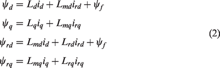
We start from Figure 1 with the stationary α–β frame, synchronously rotating d–q frame and x–y frame. The rotor has a permanent magnet with flux linkage ψ_f along the d-axis and no permanent magnetic flux along the q-axis. The aluminium plate covering the permanent magnet is represented by additional damper windings, along both d-axis (R_r and L_rd) and q-axis (R_r and L_rq) which are rotating at the rotor speed. Hence, total flux linkage along the d-axis is

ψ_{d} = L_{d} i_{d} + L_{m d} i_{r d} + ψ_{f}

and that along the q-axis is

ψ_{q} = L_{q} i_{q} + L_{m q} i_{r q}

where L_md and L_mq are mutual inductances along the two axes.

Figure 1.

Full model of the linear PMSM with damper windings.

The pole pitch is denoted by τ which is related to the instantaneous linear velocity, v, and instantaneous ω_r by the relationship, ω_r = (v/τ)π and therefore the operating frequency ω = (p/2)(v/τ)π, where p is the total number of poles of the machine. The rotor angle between the d-axis, and the α-axis, θ_r, is given by (p/2)ω_rt. The load angle, δ, is the angle between the x-axis and the d-axis.

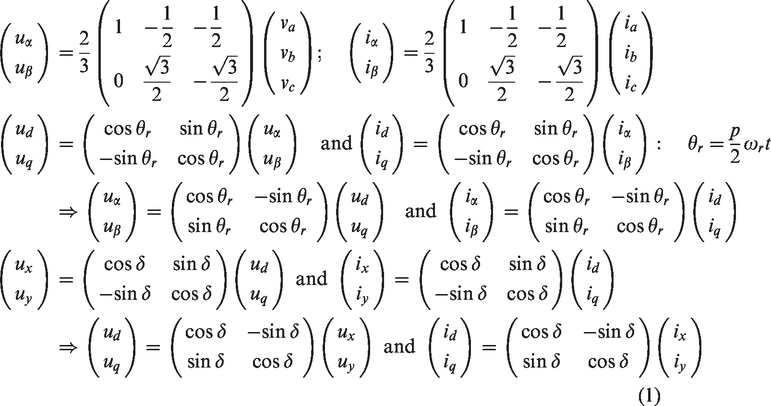
The stationary three-phase voltages, v_a, v_b, v_c are converted to the stationary α–β frame by the Clarke transformation and further converted to the rotating d–q frame (synchronous with the rotor) by the Park transformation and finally to the rotating x–y frame (synchronous with the resultant air-gap flux frame but slightly asychronous with the rotor within every control interval under the DTC mode). They are shown in equation set (1). The conversion is not only valid for voltage and current but also the flux linkage

\begin{array}{l} (\begin{matrix} u_{α} \\ u_{β} \end{matrix}) = \frac{2}{3} (\begin{array}{l} 1 - \frac{1}{2} - \frac{1}{2} \\ 0 \frac{\sqrt{3}}{2} - \frac{\sqrt{3}}{2} \end{array}) (\begin{matrix} v_{a} \\ v_{b} \\ v_{c} \end{matrix}); (\begin{matrix} i_{α} \\ i_{β} \end{matrix}) = \frac{2}{3} (\begin{array}{l} 1 - \frac{1}{2} - \frac{1}{2} \\ 0 \frac{\sqrt{3}}{2} - \frac{\sqrt{3}}{2} \end{array}) (\begin{matrix} i_{a} \\ i_{b} \\ i_{c} \end{matrix}) \\ (\begin{matrix} u_{d} \\ u_{q} \end{matrix}) = (\begin{matrix} \cos θ_{r} & \sin θ_{r} \\ - \sin θ_{r} & \cos θ_{r} \end{matrix}) (\begin{matrix} u_{α} \\ u_{β} \end{matrix}) and (\begin{matrix} i_{d} \\ i_{q} \end{matrix}) = (\begin{matrix} \cos θ_{r} & \sin θ_{r} \\ - \sin θ_{r} & \cos θ_{r} \end{matrix}) (\begin{matrix} i_{α} \\ i_{β} \end{matrix}) : θ_{r} = \frac{p}{2} ω_{r} t \\ \Rightarrow (\begin{matrix} u_{α} \\ u_{β} \end{matrix}) = (\begin{matrix} \cos θ_{r} & - \sin θ_{r} \\ \sin θ_{r} & \cos θ_{r} \end{matrix}) (\begin{matrix} u_{d} \\ u_{q} \end{matrix}) and (\begin{matrix} i_{α} \\ i_{β} \end{matrix}) = (\begin{matrix} \cos θ_{r} & - \sin θ_{r} \\ \sin θ_{r} & \cos θ_{r} \end{matrix}) (\begin{matrix} i_{d} \\ i_{q} \end{matrix}) \\ (\begin{matrix} u_{x} \\ u_{y} \end{matrix}) = (\begin{matrix} \cos δ & \sin δ \\ - \sin δ & \cos δ \end{matrix}) (\begin{matrix} u_{d} \\ u_{q} \end{matrix}) and (\begin{matrix} i_{x} \\ i_{y} \end{matrix}) = (\begin{matrix} \cos δ & \sin δ \\ - \sin δ & \cos δ \end{matrix}) (\begin{matrix} i_{d} \\ i_{q} \end{matrix}) \\ \Rightarrow (\begin{matrix} u_{d} \\ u_{q} \end{matrix}) = (\begin{matrix} \cos δ & - \sin δ \\ \sin δ & \cos δ \end{matrix}) (\begin{matrix} u_{x} \\ u_{y} \end{matrix}) and (\begin{matrix} i_{d} \\ i_{q} \end{matrix}) = (\begin{matrix} \cos δ & - \sin δ \\ \sin δ & \cos δ \end{matrix}) (\begin{matrix} i_{x} \\ i_{y} \end{matrix}) \end{array}

(1)

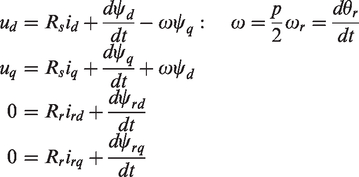
The voltage, current and flux linkage equations on the d–q frame, including the damper windings, are shown in equation set (2). ω_r is the physical rotating speed of the rotor with respect to the stator.

\begin{array}{l} u_{d} = R_{s} i_{d} + \frac{d ψ_{d}}{d t} - ω ψ_{q} : ω = \frac{p}{2} ω_{r} = \frac{d θ_{r}}{d t} \\ u_{q} = R_{s} i_{q} + \frac{d ψ_{q}}{d t} + ω ψ_{d} \\ 0 = R_{r} i_{r d} + \frac{d ψ_{r d}}{d t} \\ 0 = R_{r} i_{r q} + \frac{d ψ_{r q}}{d t} \end{array}

\begin{array}{l} ψ_{d} = L_{d} i_{d} + L_{m d} i_{r d} + ψ_{f} \\ ψ_{q} = L_{q} i_{q} + L_{m q} i_{r q} \\ ψ_{r d} = L_{m d} i_{d} + L_{r d} i_{r d} + ψ_{f} \\ ψ_{r q} = L_{m q} i_{q} + L_{r q} i_{r q} \end{array}

(2)

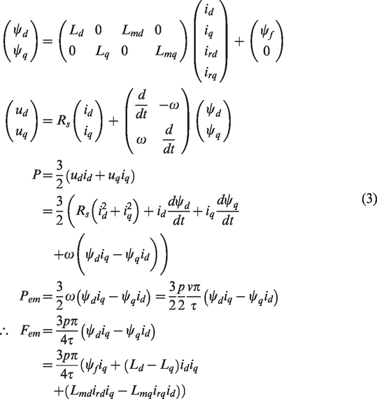
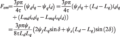
The total instantaneous power, P, is shown in equation set (3), which includes the resistive power loss, the magnetic power and the speed related electro-mechanical power, P_em. The constant (3/2) is added for energy conservation between the three-phase and two-phase systems. From P_em, the driving force F_em can be derived

\begin{array}{l} (\begin{matrix} ψ_{d} \\ ψ_{q} \end{matrix}) = (\begin{array}{l} L_{d} 0 L_{m d} 0 \\ 0 L_{q} 0 L_{m q} \end{array}) (\begin{array}{l} i_{d} \\ i_{q} \\ i_{r d} \\ i_{r q} \end{array}) + (\begin{matrix} ψ_{f} \\ 0 \end{matrix}) \\ (\begin{matrix} u_{d} \\ u_{q} \end{matrix}) = R_{s} (\begin{matrix} i_{d} \\ i_{q} \end{matrix}) + (\begin{matrix} \frac{d}{d t} & - ω \\ ω & \frac{d}{d t} \end{matrix}) (\begin{matrix} ψ_{d} \\ ψ_{q} \end{matrix}) \\ P = \frac{3}{2} (u_{d} i_{d} + u_{q} i_{q}) \\ = \frac{3}{2} (R_{s} (i_{d}^{2} + i_{q}^{2}) + i_{d} \frac{d ψ_{d}}{d t} + i_{q} \frac{d ψ_{q}}{d t} + ω (ψ_{d} i_{q} - ψ_{q} i_{d})) \\ P_{e m} = \frac{3}{2} ω (ψ_{d} i_{q} - ψ_{q} i_{d}) = \frac{3}{2} \frac{p}{2} \frac{v π}{τ} (ψ_{d} i_{q} - ψ_{q} i_{d}) \\ ∴ F_{e m} = \frac{3 p π}{4 τ} (ψ_{d} i_{q} - ψ_{q} i_{d}) \\ = \frac{3 p π}{4 τ} (ψ_{f} i_{q} + (L_{d} - L_{q}) i_{d} i_{q} + (L_{m d} i_{r d} i_{q} - L_{m q} i_{r q} i_{d})) \end{array}

(3)

To facilitate the computer simulation of such model including the damper windings, equation set (3) is re-written as equation set (4)

\begin{array}{l} u_{d} = R_{s} i_{d} + L_{d} \frac{d i_{d}}{d t} + L_{m d} \frac{d i_{r d}}{d t} - ω L_{q} i_{q} - ω L_{m q} i_{r q} \end{array}

\begin{array}{l} u_{q} = R_{s} i_{q} + L_{q} \frac{d i_{q}}{d t} + L_{m q} \frac{d i_{r q}}{d t} + ω L_{d} i_{d} \\ + ω L_{m d} i_{r d} + ω ψ_{f} \\ 0 = R_{r} i_{r d} + L_{m d} \frac{d i_{d}}{d t} + L_{r d} \frac{d i_{r d}}{d t} \\ \Rightarrow \frac{d i_{r d}}{d t} = \frac{- 1}{L_{r d}} (R_{r} i_{r d} + L_{m d} \frac{d i_{d}}{d t}) \\ 0 = R_{r} i_{r q} + L_{m q} \frac{d i_{q}}{d t} + L_{r q} \frac{d i_{r q}}{d t} \\ \Rightarrow \frac{d i_{r q}}{d t} = \frac{- 1}{L_{r q}} (R_{r} i_{r q} + L_{m q} \frac{d i_{q}}{d t}) \end{array}

(4)

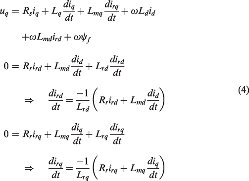
Therefore, by combining the first two and last two equations in equation set (4), equation set (5) is obtained

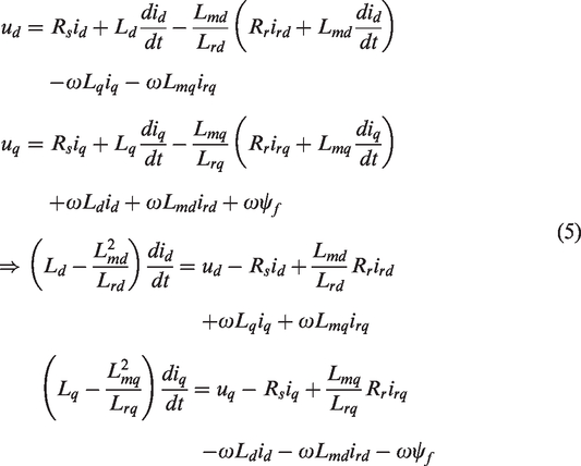
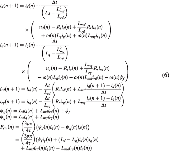
\begin{array}{l} u_{d} = R_{s} i_{d} + L_{d} \frac{d i_{d}}{d t} - \frac{L_{m d}}{L_{r d}} (R_{r} i_{r d} + L_{m d} \frac{d i_{d}}{d t}) \\ - ω L_{q} i_{q} - ω L_{m q} i_{r q} \\ u_{q} = R_{s} i_{q} + L_{q} \frac{d i_{q}}{d t} - \frac{L_{m q}}{L_{r q}} (R_{r} i_{r q} + L_{m q} \frac{d i_{q}}{d t}) \\ + ω L_{d} i_{d} + ω L_{m d} i_{r d} + ω ψ_{f} \\ \Rightarrow (L_{d} - \frac{L_{m d}^{2}}{L_{r d}}) \frac{d i_{d}}{d t} = u_{d} - R_{s} i_{d} + \frac{L_{m d}}{L_{r d}} R_{r} i_{r d} \\ + ω L_{q} i_{q} + ω L_{m q} i_{r q} \\ (L_{q} - \frac{L_{m q}^{2}}{L_{r q}}) \frac{d i_{q}}{d t} = u_{q} - R_{s} i_{q} + \frac{L_{m q}}{L_{r q}} R_{r} i_{r q} \\ - ω L_{d} i_{d} - ω L_{m d} i_{r d} - ω ψ_{f} \end{array}

(5)

The discrete form of equation set (5), at the (n + 1)th simulation interval, is shown in equation set (6), where Δt here is the simulation time interval.

\begin{array}{l} i_{d} (n + 1) = i_{d} (n) + \frac{Δ t}{(L_{d} - \frac{L_{m d}^{2}}{L_{r d}})} \times (\begin{matrix} u_{d} (n) - R_{s} i_{d} (n) + \frac{L_{m d}}{L_{r d}} R_{r} i_{r d} (n) \\ + ω (n) L_{q} i_{q} (n) + ω (n) L_{m q} i_{r q} (n) \end{matrix}) \\ i_{d} (n + 1)= i_{q} (n) + \frac{Δ t}{(L_{q} - \frac{L_{m q}^{2}}{L_{r q}})} \\ \times (\begin{matrix} u_{q} (n) - R_{s} i_{q} (n) + \frac{L_{m q}}{L_{r q}} R_{r} i_{r q} (n) \\ - ω (n) L_{d} i_{d} (n) - ω (n) L_{m d} i_{r d} (n) - ω (n) ψ_{f} \end{matrix}) \\ i_{r d} (n + 1) = i_{r d} (n) - \frac{Δ t}{L_{r d}} (R_{r} i_{r d} (n) + L_{m d} \frac{i_{d} (n + 1) - i_{d} (n)}{Δ t}) \\ i_{r q} (n + 1) = i_{r q} (n) - \frac{Δ t}{L_{r q}} (R_{r} i_{r q} (n) + L_{m q} \frac{i_{q} (n + 1) - i_{q} (n)}{Δ t}) \\ ψ_{d} (n) = L_{d} i_{d} (n) + L_{m d} i_{r d} (n) + ψ_{f} \\ ψ_{q} (n) = L_{q} i_{q} (n) + L_{m q} i_{r q} (n) \\ F_{e m} (n) = (\frac{3 p π}{4 τ}) (ψ_{d} (n) i_{q} (n) - ψ_{q} (n) i_{d} (n)) \\ = (\frac{3 p π}{4 τ}) (ψ_{f} i_{q} (n) + (L_{d} - L_{q}) i_{d} (n) i_{q} (n) \\ + L_{m d} i_{r d} (n) i_{q} (n) - L_{m q} i_{r q} (n) i_{d} (n)) \end{array}

(6)

Control by FOC

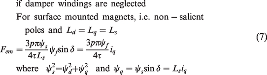
FOC is the classical control method for both induction and PMSM drives, which was also used in our previous study.^1,8 One of the pioneering applications of FOC application on lift systems could be dated back to 1992⁹ when FOC was used to control an induction motor. To work on the control methodology, the damper windings are temporarily neglected because their existence highly complicates the whole control model, i.e. the damper windings are only considered in the simulation model. Figure 2(a) shows the block diagram of control loops. From equation set (3), equation set (7) can be derived as follows

\begin{array}{l} F_{e m} = \frac{3 p π}{4 τ} (ψ_{d} i_{q} - ψ_{q} i_{d}) = \frac{3 p π}{4 τ} (ψ_{f} i_{q} + (L_{d} - L_{q}) i_{d} i_{q} \\ + (L_{m d} i_{r d} i_{q} - L_{m q} i_{r q} i_{d})) \\ = \frac{3 p π ψ_{s}}{8 τ L_{d} L_{q}} (2 ψ_{f} L_{q} \sin δ + ψ_{s} (L_{d} - L_{q}) \sin (2 δ)) \end{array}

\begin{array}{l} if damper windings are neglected \\ For surface mounted magnets, i.e. non-salient \\ poles and L_{d} = L_{q} = L_{s} \\ F_{e m} = \frac{3 p π ψ_{s}}{4 τ L_{s}} ψ_{f} \sin δ = \frac{3 p π ψ_{f}}{4 τ} i_{q} \\ where ψ_{s}^{2} = ψ_{d}^{2} + ψ_{q}^{2} and ψ_{q} = ψ_{s} \sin δ = L_{s} i_{q} \end{array}

(7)

Figure 2.

(a) Block diagram of FOC; (b) eight space vectors of PWM inverter; (c) block diagram of DFC (Conventional DTC); (d) block diagram of DSC.

The FOC control traces the instantaneous position of the d-axis in the beginning of every control interval and determines the force required, based on equation set (7), by suitably adjusting the set point of i_q, i.e. i_q (set), based on the current speed versus the required speed profile, v (set). Then, u_d and u_q are controlled according to equation set (8) (K_P and K_I are proportional and integral gains of the controllers) to arrive at the required i_d and i_q or equivalently, ψ_s and δ are so controlled to obtain the required electromechanical force. The required u_d and u_q are converted back to u_α, u_β, and finally to v_a, v_b and v_c which are generated by the appropriate pulse width modulated inverter. This method was used in So and Chan⁸

\begin{array}{l} E r (i_{q}) = i_{q} (set) - i_{q}; AccEr (i_{q}) = \sum E r (i_{q}) \\ E r (i_{d}) = i_{d} (set) - i_{d}; AccEr (i_{d}) = \sum E_{r} (i_{d}) \\ E r (v) = v (set) - v; AccEr (v) = \sum E_{r} (v) \\ i_{q} (set) = K_{P} (v) E r (v) + K_{I} (v) AccEr (v) \\ u_{q} = K_{P} (i_{q}) E r (i_{q}) + K_{I} (i_{q}) AccEr (i_{q}) \\ u_{d} = K_{P} (i_{d}) E r (i_{d}) + K_{I} (i_{d}) AccEr (i_{d}) \end{array}

(8)

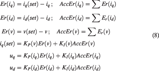
For surface-mounted magnets, i_d (set) is usually set to zero. But with saliency, a finite and constant set point for i_d was used before and confirmed effective, namely i_d(set) = –20 A, for optimal energy performance. Theoretically, for every i_q(set), there should be a corresponding i_d (set) for optimal energy consumption, as discussed in our previous article. But that naturally highly complicates the whole control process. In this article, we still adopt the constant i_d (set) approach. To follow the industry practice, i_d (set) was first constantly adjusted to 0 A.

The same speed profile for a fully loaded upward moving lift car is again considered for v (set) at any time t. The jerk, J, is consistently set to ±1.5 m/s³, acceleration/deceleration, A, consistently set to ±1 m/s² and rated speed, V, to a constant of 2.5 m/s. Therefore, t₁ = 0.7 s (jerk ends); t₂ = 2.5 s (acceleration ends); t₃ = 3.2 s (jerk ends); t₄ = 5.0 s (rated speed operation ends); t₅ = 5.7 s (jerk ends); t₆ = 7.5 s (deceleration ends); t₇ = 8.2 s (car stops). From t = 3.2 s to 5.0 s, the lift car runs under a rated speed.

Control by DTC

Direct torque control was first used in induction machine control in the late 1980s and early 1990s of the last century.^10–12 Then, the method had been applied to PMSMs.^13–16 The term, DTC, originally referred to rotary machines as ‘T’ means ‘Torque’, like induction motors and PMSMs. When DTC was used on linear PMSMs, the alphabet ‘T’ was changed to ‘Thrust’.¹⁷ In this article, DFC is used to refer to such conventional DTC on LPMSMs because a novel control mode, DSC, is newly proposed.

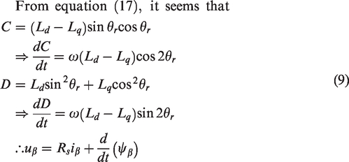
Again, to implement the control practically, the contribution by the damper windings is temporarily neglected in the control loops but it is included in the simulation model to test whether our control can effectively do the job. The force equation of equation set (3) is re-visited here but we are looking at the x–y frame. Therefore, the co-ordinate conversion from the d–q frame to the x–y frame as indicated in equation set (1) is used. They are shown in equation set (9).

\begin{array}{l} (\begin{matrix} u_{d} \\ u_{q} \end{matrix}) = (\begin{matrix} \cos δ & - \sin δ \\ \sin δ & \cos δ \end{matrix}) (\begin{matrix} u_{x} \\ u_{y} \end{matrix}) and \\ (\begin{matrix} i_{d} \\ i_{q} \end{matrix}) = (\begin{matrix} \cos δ & - \sin δ \\ \sin δ & \cos δ \end{matrix}) (\begin{matrix} i_{x} \\ i_{y} \end{matrix}) \end{array}

\begin{array}{l} ψ_{d} = ψ_{s} \cos δ and ψ_{q} = ψ_{s} \sin δ \\ F_{e m} = \frac{3 p π}{4 τ} (ψ_{d} i_{q} - ψ_{q} i_{d}) \\ = \frac{3 p π}{4 τ} [ψ_{s} \cos δ (i_{x} \sin δ + i_{y} \cos δ) \\ - ψ_{s} \sin δ (i_{x} \cos δ - i_{y} \sin δ)] \\ = \frac{3 p π}{4 τ} (ψ_{s} i_{y}) \end{array}

(9)

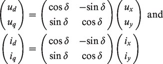
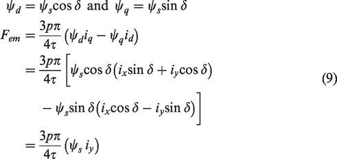
It appears from equation set (9) that the force can either be controlled by the air-gap flux linkage or by i_y. By DTC approach, ψ_s is the target under control to adjust the force because i_y can be absorbed into the variation of δ, as shown by the derivation below.

By converting the first equation in equation set (3) to the x–y frame by using the second last equation in equation set (1) and ignoring the damper windings, we have

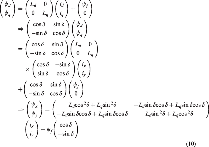
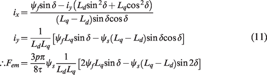
\begin{array}{l} (\begin{matrix} ψ_{d} \\ ψ_{q} \end{matrix}) = (\begin{matrix} L_{d} & 0 \\ 0 & L_{q} \end{matrix}) (\begin{matrix} i_{d} \\ i_{q} \end{matrix}) + (\begin{matrix} ψ_{f} \\ 0 \end{matrix}) \\ \Rightarrow (\begin{matrix} \cos δ & \sin δ \\ - \sin δ & \cos δ \end{matrix}) (\begin{matrix} ψ_{d} \\ ψ_{q} \end{matrix}) = (\begin{matrix} \cos δ & \sin δ \\ - \sin δ & \cos δ \end{matrix}) (\begin{matrix} L_{d} & 0 \\ 0 & L_{q} \end{matrix}) (\begin{matrix} \cos δ & - \sin δ \\ \sin δ & \cos δ \end{matrix}) (\begin{matrix} i_{x} \\ i_{y} \end{matrix}) \\ + (\begin{matrix} \cos δ & \sin δ \\ - \sin δ & \cos δ \end{matrix}) (\begin{matrix} ψ_{f} \\ 0 \end{matrix}) \\ \Rightarrow (\begin{matrix} ψ_{x} \\ ψ_{y} \end{matrix}) = (\begin{matrix} L_{d} \cos^{2} δ + L_{q} \sin^{2} δ - L_{d} \sin δ \cos δ + L_{q} \sin δ \cos δ \\ - L_{d} \sin δ \cos δ + L_{q} \sin δ \cos δ L_{d} \sin^{2} δ + L_{q} \cos^{2} δ \end{matrix}) (\begin{matrix} i_{x} \\ i_{y} \end{matrix}) + ψ_{f} (\begin{matrix} \cos δ \\ - \sin δ \end{matrix}) \end{array}

(10)

Readers please note that the damper windings are considered in all simulation loops but not in the control loops in order to simplify the control equations. As a matter of fact, the x-axis is the axis of the resultant air-gap flux linkage, i.e. ψ_s = ψ_x, and naturally, there is no resultant air-gap flux linkage along the y-axis, implying that ψ_y = 0. Putting this into the last equation of equation set (10), it is possible to get i_x and i_y with respect to ψ_s and δ and the final force with reference to the last equation in equation set (9), as shown in equation set (11).

\begin{array}{l} i_{x} = \frac{ψ_{f} \sin δ - i_{y} (L_{d} \sin^{2} δ + L_{q} \cos^{2} δ)}{(L_{q} - L_{d}^{}) \sin δ \cos δ} \\ i_{y} = \frac{1}{L_{d} L_{q}} [ψ_{f} L_{q} \sin δ - ψ_{s} (L_{q} - L_{d}) \sin δ \cos δ] \\ ∴ F_{e m} = \frac{3 p π}{8 τ} ψ_{s} \frac{1}{L_{d} L_{q}} [2 ψ_{f} L_{q} \sin δ - ψ_{s} (L_{q} - L_{d}) \sin 2 δ] \end{array}

(11)

which is the same as in equation set (7).

Control by DFC

Here, DFC is the term used to refer to the conventional DTC applied to, in our case, a LPMSM. We have to work on the stationary α–β frame to estimate ψ_α, ψ_β, and hence ψ_s as in equation set (9) because one DFC’s significant advantage is that no co-ordinate transformation to the d–q frame is needed to facilitate the control process. The control is thus simpler to implement on electronic circuitry. By DFC, we need to estimate the air-gap flux linkages by measuring the stator currents, i_α and i_β, along the α- and β-axes, respectively.

The standard control procedure¹⁷ of DTC (or DFC in this article) is shown below. What can be actuated are the three-phase voltages from the inverter, v_a, v_b and v_c, which could be converted to u_α, u_β, as in equation set (1). By measuring the instantaneous three-phase currents, i_a, i_b and i_c, actually, only two are required because of the Kirchoff’s current law, and by converting them into i_α and i_β, it is possible to trace ψ_α and ψ_β as shown in equation set (12) and then estimate the electromechanical driving force of the motor

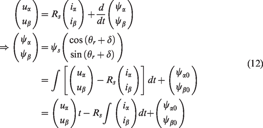
\begin{array}{l} (\begin{matrix} u_{α} \\ u_{β} \end{matrix}) = R_{s} (\begin{matrix} i_{α} \\ i_{β} \end{matrix}) + \frac{d}{d t} (\begin{matrix} ψ_{α} \\ ψ_{β} \end{matrix}) \\ \Rightarrow (\begin{matrix} ψ_{α} \\ ψ_{β} \end{matrix}) = ψ_{s} (\begin{matrix} \cos (θ_{r} + δ) \\ \sin (θ_{r} + δ) \end{matrix}) \\ = \int [(\begin{matrix} u_{α} \\ u_{β} \end{matrix}) - R_{s} (\begin{matrix} i_{α} \\ i_{β} \end{matrix})] d t + (\begin{matrix} ψ_{α 0} \\ ψ_{β 0} \end{matrix}) \\ = (\begin{matrix} u_{α} \\ u_{β} \end{matrix}) t - R_{s} \int (\begin{matrix} i_{α} \\ i_{β} \end{matrix}) d t + (\begin{matrix} ψ_{α 0} \\ ψ_{β 0} \end{matrix}) \end{array}

(12)

At time t = 0, it is assumed that the d-axis aligns with the α-axis and thus ψ_α₀ = ψ_f and ψ_β₀ = 0. Literature usually states that R_s is very small, and hence the rate of change of ψ_α and ψ_β is somehow directly proportional to u_α and u_β which are constants in every control interval. Our simulation experience revealed that, in the beginning, the two flux linkages could be estimated quite accurately. But as time went on, the accumulated error became so big that control started to go unstable. If the rotor position is known by measurement or by estimation, the following equation (13) could be used to estimate the flux linkages directly once the currents can be measured, without the use of continuous integration, provided that L_d = L_q = L_s, i.e. no saliency

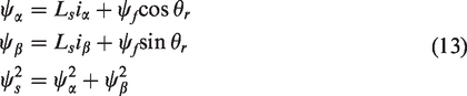
\begin{array}{l} ψ_{α} = L_{s} i_{α} + ψ_{f} \cos θ_{r} \\ ψ_{β} = L_{s} i_{β} + ψ_{f} \sin θ_{r} \\ ψ_{s}^{2} = ψ_{α}^{2} + ψ_{β}^{2} \end{array}

(13)

In fact, the instantaneous speed, ω_r, of the motor has to be continuously monitored for precise motion control of a lift car, anyway. In other words, θ_r is also continuously monitored. As a matter of fact, modern encoders to serve the function of tachometers actually count pulses as the rotor moves and differentiate them into speed.

As seen in equation set (13), it is only valid when surface-mounted permanent magnets are used, i.e. no saliency. With saliency when L_d ≠ L_q, new expressions for the flux linkages are required. We worked backward from the d–q frame to the α–β frame without considering the damper windings again. Parts of equation sets (1) and (2) are combined as shown in equation set (14). Here, φ could refer to u, i or ψ

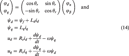
(\begin{matrix} φ_{d} \\ φ_{q} \end{matrix}) = (\begin{matrix} \cos θ_{r} & \sin θ_{r} \\ - \sin θ_{r} & \cos θ_{r} \end{matrix}) (\begin{matrix} φ_{α} \\ φ_{β} \end{matrix}) and \begin{array}{l} ψ_{d} = ψ_{f} + L_{d} i_{d} \\ ψ_{q} = L_{q} i_{q} \\ u_{d} = R_{s} i_{d} + \frac{d ψ_{d}}{d t} - ω ψ_{q} \\ u_{q} = R_{s} i_{q} + \frac{d ψ_{q}}{d t} + ω ψ_{d} \end{array}

(14)

From equation set (14), equation sets (15), (16) and (17) can be derived

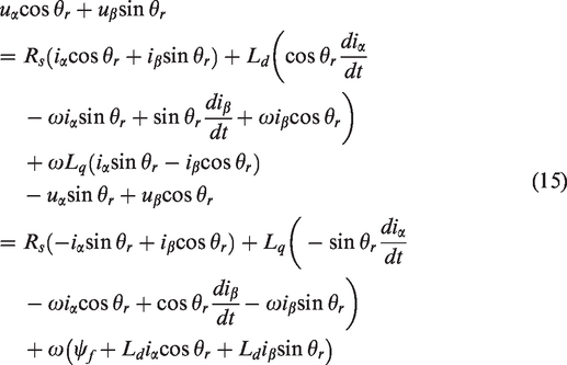
\begin{array}{l} u_{α} \cos θ_{r} + u_{β} \sin θ_{r} \\ = R_{s} (i_{α} \cos θ_{r} + i_{β} \sin θ_{r}) + L_{d} (\cos θ_{r} \frac{d i_{α}}{d t} \\ - ω i_{α} \sin θ_{r} + \sin θ_{r} \frac{d i_{β}}{d t} + ω i_{β} \cos θ_{r}) \\ + ω L_{q} (i_{α} \sin θ_{r} - i_{β} \cos θ_{r}) \\ - u_{α} \sin θ_{r} + u_{β} \cos θ_{r} \\ = R_{s} (- i_{α} \sin θ_{r} + i_{β} \cos θ_{r}) + L_{q} (- \sin θ_{r} \frac{d i_{α}}{d t} \\ - ω i_{α} \cos θ_{r} + \cos θ_{r} \frac{d i_{β}}{d t} - ω i_{β} \sin θ_{r}) \\ + ω (ψ_{f} + L_{d} i_{α} \cos θ_{r} + L_{d} i_{β} \sin θ_{r}) \end{array}

(15)

By combining the two equations of (15) and eliminating either u_α or u_β

\begin{array}{l} u_{α} = R_{s} i_{α} + (L_{d} \cos^{2} θ_{r} + L_{q} \sin^{2} θ_{r}) \frac{d i_{α}}{d t} \\ + (L_{d} - L_{q}) \sin θ_{r} \cos θ_{r} \frac{d i_{β}}{d t} \\ - ω i_{α} (L_{d} - L_{q}) \sin 2 θ_{r} \\ + ω i_{β} (L_{d} - L_{q}) \cos 2 θ_{r} - ω ψ_{f} \sin θ_{r} \\ = R_{s} i_{α} + (L_{s}) \frac{d i_{α}}{d t} - ω ψ_{f} sin θ_{r} \\ only  with  no saliency \\ = R_{s} i_{α} + \frac{d}{d t} (L_{s} i_{α} + ψ_{f} \cos θ_{r}) = R_{s} i_{α} + \frac{d ψ_{α}}{d t} \end{array}

(16)

\begin{array}{l} u_{β} = R_{s} i_{β} + (L_{d} - L_{q}) \sin θ_{r} \cos θ_{r} \frac{d i_{α}}{d t} \\ + (L_{d} \sin^{2} θ_{r} + L_{q} \cos^{2} θ_{r}) \frac{d i_{β}}{d t} \\ + ω i_{α} (L_{d} - L_{q}) \cos 2 θ_{r} \\ + ω i_{β} (L_{d} - L_{q}) \sin 2 θ_{r} + ω ψ_{f} \cos θ_{r} \\ = R_{s} i_{β} + (L_{s}) \frac{d i_{β}}{d t} + ω ψ_{f} \cos θ_{r} \\ only with no saliency \\ = R_{s} i_{β} + \frac{d}{d t} (L_{s} i_{β} + ψ_{f} \sin θ_{r}) = R_{s} i_{β} + \frac{d ψ_{β}}{d t} \end{array}

(17)

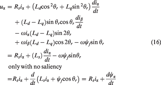
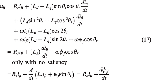
From equation sets (16) and (17), without saliency, they are equivalent to equation set (13). With saliency, the stationary voltage–current equations are not that simple anymore as the two orthogonal stator windings are not independent of each other, i.e. they are magnetically coupled to each other.

When L_d ≠ L_q, we can derive the two stationary flux linkages with two new expressions as shown in equation set (18)

\begin{array}{l} Let ψ_{α} = A i_{α} + B i_{β} + ψ_{f} \cos θ_{r} and \\ ψ_{β} = C i_{α} + D i_{β} + ψ_{f} \sin θ_{r} \\ From equation (16), it seems that \\ A = L_{d} \cos 2 θ_{r} + L_{q} \sin 2 θ_{r} \\ \Rightarrow \frac{d A}{d t} = - ω (L_{d} - L_{q}) \sin 2 θ_{r} \end{array}

\begin{array}{l} B = (L_{d} - L_{q}) \sin θ_{r} \cos θ_{r} \\ \Rightarrow \frac{d B}{d t} = ω (L_{d} - L_{q}) \cos 2 θ_{r} \\ ∴ u_{α} = R_{s} i_{α} + \frac{d}{d t} (ψ_{α}) \end{array}

(18)

\begin{array}{l} From equation (17), it seems that \\ C = (L_{d} - L_{q}) \sin θ_{r} \cos θ_{r} \\ \Rightarrow \frac{d C}{d t} = ω (L_{d} - L_{q}) \cos 2 θ_{r} \\ D = L_{d} \sin 2 θ_{r} + L_{q} \cos 2 θ_{r} \\ \Rightarrow \frac{d D}{d t} = ω (L_{d} - L_{q}) \sin 2 θ_{r} \\ ∴ u_{β} = R_{s} i_{β} + \frac{d}{d t} (ψ_{β}) \end{array}

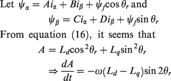
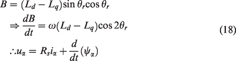
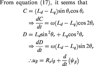
Therefore, equation (12) can still be used with saliency but the two stationary flux linkages have to be defined differently. In this way, the accumulated error to estimate the flux linkages can be removed while they can be calculated analytically by knowing i_α, i_β, ψ_f and θ_r.

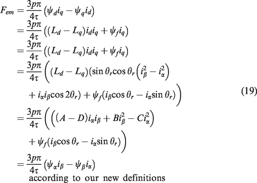
To verify that such new definitions are correct, it is straight forward to convert all parameters from the α–β frame back to the d–q frame. One more advantage is that it is possible to estimate the instantaneous driving force directly on the α–β frame, as shown below. From equation set (9) and the new expressions of the flux linkages

\begin{array}{l} F_{e m} = \frac{3 p π}{4 τ} (ψ_{d} i_{q} - ψ_{q} i_{d}) \\ = \frac{3 p π}{4 τ} ((L_{d} - L_{q}) i_{d} i_{q} + ψ_{f} i_{q}) \\ = \frac{3 p π}{4 τ} ((L_{d} - L_{q}) i_{d} i_{q} + ψ_{f} i_{q}) \\ = \frac{3 p π}{4 τ} ((L_{d} - L_{q}) (\sin θ_{r} \cos θ_{r} (i_{β}^{2} - i_{α}^{2}) \\ + i_{α} i_{β} \cos 2 θ_{r}) + ψ_{f} (i_{β} \cos θ_{r} - i_{α} \sin θ_{r})) \\ = \frac{3 p π}{4 τ} (((A - D) i_{α} i_{β} + B i_{β}^{2} - C i_{α}^{2}) + ψ_{f} (i_{β} \cos θ_{r} - i_{α} \sin θ_{r})) \\ = \frac{3 p π}{4 τ} (ψ_{α} i_{β} - ψ_{β} i_{α}) \\ according to our new definitions \end{array}

(19)

What are to be controlled are the instantaneous changes of ψ_α and ψ_β either by continuous integration (with error but simpler) or by our new definitions (without error). To implement that, a two-level inverter with three bridges (A, B and C) is used. N is the negative bus; V_dc is voltage of the positive bus. The neutral point of the star-connected motor load is n. V_nN is the voltage between the neutral point of the star-connected motor load and the negative bus of the inverter. v_a (0°), v_b (+120°) and v_c (–120°) are voltages across the three star-connected load terminals of the motor and their neutral point.

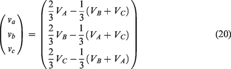
V_A is the voltage at the junction between two power switching devices of bridge A with respect to N. Therefore, V_A = v_a + V_nN, V_B = v_b + V_nN and V_C = v_c + V_nN. For a star-connected load, it is always assumed that v_a + v_b + v_c = 0, and therefore V_nN = 1/3(V_A + V_B + V_C). Therefore, equation (20) is valid

(\begin{matrix} v_{a} \\ v_{b} \\ v_{c} \end{matrix}) = (\begin{matrix} \frac{2}{3} V_{A} - \frac{1}{3} (V_{B} + V_{C}) \\ \frac{2}{3} V_{B} - \frac{1}{3} (V_{A} + V_{C}) \\ \frac{2}{3} V_{C} - \frac{1}{3} (V_{B} + V_{A}) \end{matrix})

(20)

When the upper switching device of bridge A is on, V_A = V_dc and if the lower switch of bridge A is on, V_A = 0 and so on. So, the following table, Table 1, can be formulated. Here, V₁(1,0,0) means the upper switch of the first bridge, A, is on and the lower switches of the remaining bridges are on. Either the upper or the lower switch has to be turned on anytime, but not both. The space vector pulse width modulation inverter is shown in Figure 2(b). Sector j (j running from 1 to 6) spans a range of angles equal to [(2j – 3) × π/6, (2j – 1) × π/6]. Altogether, there are eight space vectors while V₇ and V₈ have no effect on the motor.

Table 1.

Eight space vectors of the two-level inverter.

Switching sequence	v_a	v_b	v_c
V₁ (1,0,0)	(2/3) V_dc	–(1/3) V_dc	–(1/3) V_dc
V₂ (1,1,0)	(1/3) V_dc	(1/3) V_dc	–(2/3) V_dc
V₃ (0,1,0)	–(1/3) V_dc	(2/3) V_dc	–(1/3) V_dc
V₄ (0,1,1)	–(2/3) V_dc	(1/3) V_dc	(1/3) V_dc
V₅ (0,0,1)	–(1/3) V_dc	–(1/3) V_dc	(2/3) V_dc
V₆ (1,0,1)	(1/3) V_dc	–(2/3) V_dc	(1/3) V_dc
V₇ (0,0,0)	0	0	0
V₈ (1,1,1)	0	0	0

Once the three-phase voltages are determined by the appropriate switching sequence, they are first converted to u_α (0°) and u_β (+90°) by equation (21)

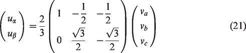
(\begin{matrix} u_{α} \\ u_{β} \end{matrix}) = \frac{2}{3} (\begin{array}{l} 1 - \frac{1}{2} - \frac{1}{2} \\ 0 \frac{\sqrt{3}}{2} - \frac{\sqrt{3}}{2} \end{array}) (\begin{matrix} v_{a} \\ v_{b} \\ v_{c} \end{matrix})

(21)

Table 1 is extended to include u_α and u_β by equation (21), as shown in Table 2.

Table 2.

Eight space vectors of a two-level inverter including u_α and u_β.

Switching sequence	v_a	v_b	v_c	u_α	u_β
V₁ (1,0,0)	(2/3) V_dc	–(1/3) V_dc	–(1/3) V_dc	(2/3) V_dc	0
V₂ (1,1,0)	(1/3) V_dc	(1/3) V_dc	–(2/3) V_dc	(1/3) V_dc	$1 / \sqrt{3}$ V_dc
V₃ (0,1,0)	–(1/3) V_dc	(2/3) V_dc	–(1/3) V_dc	–(1/3) V_dc	$1 / \sqrt{3}$ V_dc
V₄ (0,1,1)	–(2/3) V_dc	(1/3) V_dc	(1/3) V_dc	–(2/3) V_dc	0
V₅ (0,0,1)	–(1/3) V_dc	–(1/3) V_dc	(2/3) V_dc	–(1/3) V_dc	$- 1 / \sqrt{3}$ V_dc
V₆ (1,0,1)	(1/3) V_dc	–(2/3) V_dc	(1/3) V_dc	(1/3) V_dc	$- 1 / \sqrt{3}$ V_dc
V₇ (0,0,0)	0	0	0	0	0
V₈ (1,1,1)	0	0	0	0	0

These two orthogonal stationary phase voltages are applied to the simulation model to arrive at i_d, i_q and θ_r then i_α, i_β to produce ψ_α, ψ_β and thus ψ_s and F_em by equation (19) in the control model.

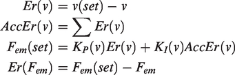
In DFC, a speed PI controller and two hysteresis controllers (one for force and one for magnetic flux) are needed, i.e. totally three in number. The speed controller helps to adjust the set point of the force controller, and the force controller adjusts δ within each control interval. They are described below and shown in Figure 2(c). It can be seen that the real-time force, F_em, has to be computed from time to time based on equation (19).

\begin{array}{l} E r (v) = v (set) - v \\ A ccEr (v) = \sum E r (v) \\ F_{e m} (set) = K_{P} (v) E r (v) + K_{I} (v) AccEr (v) \\ E r (F_{e m}) = F_{e m} (set) - F_{e m} \end{array}

\begin{array}{l} ε (F_{e m}) = {\begin{matrix} + 1 to increase F_{e m} (i.e. δ) if E r (F_{e m}) > + Δ F \\ - 1 to reduce F_{e m} (i.e. δ) if E r (F_{e m}) < - Δ F \end{matrix}} \\ with hysteresis band \\ E r (ψ_{s}) = ψ_{s} (set) - ψ_{s} \\ ε (ψ_{s}) = {\begin{matrix} + 1 to increase ψ_{s} if E r (ψ_{s}) > + Δ ψ \\ - 1 to reduce ψ_{s} if E r (ψ_{s}) < - Δ ψ \end{matrix}} \\ with hysteresis band \end{array}

(22)

ψ_s (set) was obtained from the FOC control history, and it was found to be around 115–120% of ψ_f. Table 3 ¹⁸ is used to determine which of the six space vectors are to be employed when the instantaneous ψ_s is in the jth sector. That explains why it is important to estimate ψ_s analytically, in particular, when L_d ≠ L_q.

Table 3.

Switching table to generate V(n) at the nth control interval.

V (n – 1) in the jth sector		F_em or δ control
V (n – 1) in the jth sector		ε (F_em) = +1	ε (F_em) = –1
ψ_s control	ε (ψ_s) = +1	j + 1	j – 1
ψ_s control	ε (ψ_s) = –1	j + 2	j – 2

Control by DSC

In the previous conventional control, three controllers are needed. The instantaneous F_em has to be computed by measuring i_α and i_β. A new and simpler method is proposed here, shown in equation set (23), where only two hysteresis controllers are needed. The control loops are shown in Figure 2(d). The instantaneous speed of the rotor, v, is measured, and this is used to directly control δ. Then, ψ_s is being controlled within a range [ψ_s(set) – Δψ, ψ_s(set) + Δψ]. The major demand of DFC and DSC is that the control interval has to be very short as compared with that of FOC. Therefore, simple hardware and software design is necessary for cost-effective implementation.

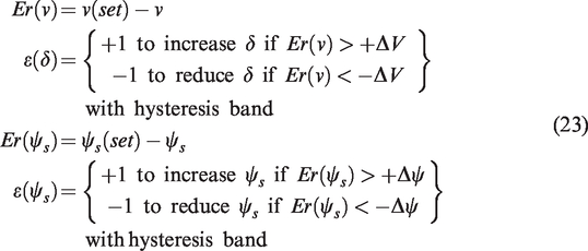
\begin{array}{l} E r (v) = v (set) - v \\ ε (δ) = {\begin{matrix} + 1 to increase δ if E r (v)>+ Δ V \\ - 1 to reduce δ if E r (v) < - Δ V \end{matrix}} \\ with hysteresis band \\ E r (ψ_{s}) = ψ_{s} (set) - ψ_{s} \\ ε (ψ_{s}) = {\begin{matrix} + 1 to increase ψ_{s} if E r (ψ_{s}) > + Δ ψ \\ - 1 to reduce ψ_{s} if E r (ψ_{s}) < - Δ ψ \end{matrix}} \\ with  hysteresis band \end{array}

(23)

Though DSC is simple, it will later be shown that its control is less precise as compared with that of DFC.

Imperfections to consider and parameters for simulation

For completeness and easy reference, all imperfections considered in the last article⁸ are quickly reviewed here. Friction is the combination of velocity independent Coulomb friction, the velocity-dependent viscous friction and the Stribeck friction. They are shown in equation (24) for quick reference. C_fr is the coefficient of Coulomb friction, V_fr the coefficient of the viscous friction, S_fr the coefficient of the Stribeck friction, k_fr the coefficient of the order of velocity in Stribeck friction and v the instantaneous velocity of the lift car

Friction = C_{f r} s ign (v) + V_{f r} v + sign (v) S_{f r} e^{- k_{f r} | v |}

(24)

Next, the cogging force is considered, as shown in equation (25). F_cog can be modelled by sinusoidal functions of the mover position, df, from a fixed reference point along the hoistway with periods of φ₁ and φ₂ and amplitudes of K_sc, A_r₁ _c and A_r₂ _c

\begin{array}{l} F_{cog} = K_{s c} \sin (φ_{1}^{} * xcog * 2 π) \\ \times (A_{r 1 c} + A_{r 2 c} \sin (φ_{2} * xcog * 2 π)) \\ where xcog = \mod (d f, τ) \end{array}

(25)

Owing to the limited length of the mover, the phenomenon of end-effect exists, as shown in equation (26)

F_{end - effect} = ξ (t) F_{e m} where  0< ξ (t)<1

(26)

In this simulation, ξ(t) is constantly set to 0.01, as in the previous paper.

Having taken into account of all the imperfections, the following force equation (27) is used throughout the simulation intervals

\begin{array}{l} F_{e m} = m c * g + m c * \frac{d v}{d t} + Friction \\ + F_{cog} + F_{end - effect} \end{array}

(27)

where mc = mass of elevator car including full load, and g = gravitational constant=9.81 m/s²

In this paper, some parameters used in the previous paper are adopted again with some modifications and additions, as shown in Table 4. It must be noted that the simulation model is consistent under all three modes of control: FOC, DFC and DSC. Here, t_c refers to the control model and t_s to the simulation model.

Table 4.

Values of parameters used in the simulations.

R_s (Ω)	0.2	L_q/L_d (mH/mH)	4.0/2.0	C_fr (N)	300.0
ψ_f (Wb)	0.4	P	16	V_fr (Ns/m)	10.0
L_md (mH)	0.1	L_mq (mH)	0.2	R_r (Ω)	0.05
τ (m)	0.1	mc (kg)	2000	S_fr (N)	100.0
v (m/s) rated	2.5	g (m/s²)	9.81	k_fr (s/m)	30.0
K_sc	0.7	φ₁ (1/m)	41.0	φ₂ (1/m)	4.0
A_r₁ _c (N)	130.0	A_r₂ _c (N)	45.0	ξ	0.01
K_P(i_d) – FOC	0.5	K_I(i_d) – FOC	1.0	K_P(i_q) – FOC	1.0
K_I(i_q) – FOC	0.25	K_P(v) – FOC	2000.0	K_I(v) – FOC	25.0
Δt_c (μs) – FOC	500.0	Δt_s (μs) – FOC	50.0
Δt_c (μs) – DFC & DSC	50.0	Δt_s (μs) – DFC & DSC	10.0
K_P(v) – DFC	20,000.0	K_I(v) – DFC	250.0	ψ_s(set) (Wb) – DFC	0.5
Δψ (Wb) – DFC	0.005	ΔF (N) – DFC	50.0
ΔV (m/s) – DSC	0.05	ψ_s(set) (Wb) – DSC	0.5	Δψ (Wb) – DSC	0.005

Results of simulations

Accuracy of speed control

Figure 3(a) shows a comparison of the performance between all three types of control. If reference was made to the exact speed profile, all three exhibited more or less the same profile as originally designed. Then, the deviation of the exact speed from the designed speed is considered.

Figure 3.

(a) Comparison of speed control performance – whole journey; (b) comparison of speed control performance – rated speed.

It can be seen that FOC could provide the best performance in general. The performance of DFC was poorest during start-up and stopping while there was a constant speed error under DSC, which will be further discussed in the next section. During the period of rated speed operation, as seen in Figure 3(b), the speed deviation was only around ±0.0005 m/s versus a rated speed of 2.5 m/s for FOC. The speed deviation under DFC was even smaller, perhaps due to the existence of the speed controller that provides real-time driving force setting.

For DSC, a constant real-time speed error was always seen, with a deviation around 0.05 m/s. That could be due to the absence of a PI speed controller. Having said that, the speed control was smoother than that of DFC.

Start-up force consideration

From Figure 3, it can be seen that the speed performance was not satisfactory during the start-up period of a fractional second long for all three types of control though that of DFC was the worse. Reference is made to Figure 4 where F_em was plotted during the start-up period from t = 0 to 0.5 s.

Figure 4.

Start-up force consideration.

It is obvious that FOC could give the best driving force performance where instability only occurred during the first 0.02 s, and the stable 20 kN upward force could be seen after that with a gradual increase to accelerate the lift car upward. DFC was the worst out of three where stability could more or less be attained at 0.5 s after start-up. DSC was also unstable during the first 0.1 s but small vibration was expected after that though the average increase in force was more or less the same as that of FOC.

A more detailed investigation into the two curves belonging to DFC and DSC revealed that the upward driving force could get down to 7 and 10 kN by 0.04–0.05 s after start-up. It should be noted that there was always a 20-kN gravitational force pulling the lift car downward. When the upward force fell below this value, the car would fall instead of moving upward. Although the controllers are still capable of responding quickly and driving the load upwards, the riding comfort would be very poor and will be felt by the passengers.

To solve this problem when using DFC or DSC, one way is to hold the brake during the period of initial instability. However, the brake has to be equipped with a force sensor, which should not be released until the net upward force on the lift car is non-zero and is stable for a period of say 0.2 s or longer. That is to make sure the lift car only goes upward under the desirable jerk and acceleration once the brake is released.

Power consumption

Power or energy consumption has been the key performance index of most engineering systems, which was considered significantly in our two previous articles. Figure 5 shows the different power consumption profiles under the three types of control.

Figure 5.

Power consumption consideration.

It is expected that the power consumption profile of FOC was the best, the smoothest out of three. Such profile was also depicted in the two previous articles. The consumption was highest during the second jerk of the acceleration period.

As expected from the speed profiles shown in Figure 3, the power consumption profiles of DFC and DSC were rather rough and bumpy. It is reasonable to assume that the current profiles of these two control modes were also bumpy, which was not good to the circuitry from the maintenance point of view.

Regarding the overall energy consumption of the whole fully loaded up journey, FOC consumed 295.6 kJ; DFC consumed 276.2 kJ; DSC consumed 291.1 kJ. That means the energy consumption of FOC was the highest while the direct torque control mode could consume slightly less by sacrificing riding comfort and precise speed control. That was due to the simple choice of i_d(set) = 0 A. In order to show the argument is valid, one more simulation was carried out on FOC using i_d(set) = –20 A as in the previous article.⁸ Figure 6 shows the new power consumption and the speed error. It can be seen that both the power consumed and speed error were slightly reduced. The total energy consumption became 288.9 kJ which was lower than that of DSC.

Figure 6.

Power consumption and speed error under FOC with i_d(set) = –20 A.

Stationary magnetic flux estimation

One new discovery stated in this article is the analytical estimation of the two stationary magnetic fluxes, namely ψ_α and ψ_β, respectively. Traditionally, in other literature, such two values were estimated by integration based on real-time voltages, u_α and u_β, and real-time currents, i_α and i_β, as shown in equation set (12). They could analytically be estimated by equation set (13), provided that surface-mounted magnets were used, i.e. no saliency. When L_d ≠ L_q, the only way to estimate ψ_α and ψ_β is using continuous integration as discussed in almost all traditional articles. But we are all aware that error due to integration, in particular, those related to the initial values has been accumulating. So, the error of these two flux linkages may be too large to be acceptable as time goes by, say towards the end of a journey. In this article, a new definition for ψ_α and ψ_β has been proposed in equation set (18), so that both values can be analytically estimated by knowing i_α, i_β and θ_r, respectively. No continuous integration is deemed necessary anymore. The two methods are compared in Figure 7 where the exact differences between the two values are depicted.

Figure 7.

Stationary magnetic flux estimation.

It can be seen that for most of the time, the exact differences are within a boundary of ±0.002 Wb while we are talking about a usual value of flux linkages within a range of [0.2 Wb, 0.7 Wb]. Therefore, the new definition agrees well with the traditional method of integration. Obviously, the new definition can give a more accurate estimation because it is analytical. And this works well when salient magnetic poles exist.

A quick comparison

Table 5 gives a quick and qualitative comparison between the three types of control methods, namely FOC, DFC and DSC.

Table 5.

Comparison of performance between FOC, DFC and DSC.

Feature	FOC	DFC	DSC
Start-up control	Good	Poorest	Poor
Accuracy of speed control	Good	Good	Poor
Current profile	Smooth	Rough	Rough
Magnetic flux estimation	Not applicable	Poor with saliency, but satisfactory by our novel method	Poor with saliency, but satisfactory by our novel method
Energy consumption	Fair	Best	Better
Circuit complication	Complicated (3 controllers)	Complicated (3 controllers)	Simpler (2 controllers)
Demand of speed of operation of control processors	Low	High	High
Power electronics components	Low cost IGBTs	High cost MOSFETs	High cost MOSFETs

Conclusion

A comprehensive model of a linear permanent magnet synchronous machine with all common imperfection has been considered and simulated, including pole saliency, the existence of the aluminium cover represented by induction windings on the rotor, different types of friction, cogging force and end effect. Based on this machine model, three types of control have been implemented and studied by simulation, including FOC and two under the category of DTC, namely the DFC and DSC, on a typical full-loaded upward journey of a ropeless lift car. DSC is one new control method proposed in this article for lift operation, as compared with conventional DTC implementation.

Regarding accuracy of speed control, the simulation reveals that FOC could provide a relatively smooth speed profile involving jerk, acceleration, rated speed operation, jerk and deceleration, over the whole journey while the other two have some shortcomings. The start-up performance of DFC is poorest, which has a major implication on riding comfort of human passengers who are quite sensitive to shaking or vibration during the journey. The poorer speed control is significant, in particular, during the initial start-up process a second long. DSC cannot maintain the desirable speed operation as there is always a permanent error.

A more detailed investigation into the start-up process reveals that the driving force fluctuation is rather serious during the first half a second under DFC or DSC, DFC in particular. If the brake is released at time t = 0 s, there is a chance that the control cannot catch up with the falling motion of the lift car because the minimum uplift force has to be equal to the dead weight of the car, i.e. 20 kN in our simulation. Our controllers were fine tuned in the simulation, and therefore the car did not fall but the risk is high under other conditions. One solution suggested here is the installation of a force sensor on the brake, so that it is only released when the driving force is 20 kN or higher for a certain period of time. FOC can produce the required magnetic flux linkages almost instantly while DFC and DSC need time to build up the flux linkages by integration. That may explain why the start-up performance of FOC is much better.

Regarding energy consumption, it is a surprise that both DFC and DSC consume a little bit less energy as compared with that of FOC. That may be due to the fact that something has to be sacrificed to gain riding comfort, or else, our FOC controllers’ settings have not been tuned optimal. In advanced FOC, i_d should not be constant as it should be i_q (governing the driving torque) dependent. In our simulation, to be more realistic and practical, a zero i_d setting normally used in the industry has been used throughout. That may explain why the consumption of FOC is slightly higher. To verify the argument, another simulation was carried out by using –20 A as the i_d setting, and a small reduction in the energy consumption was found.

Another new finding in this article is the analytical computation of the two magnetic flux linkages along the stationary α- and β-axes. Conventionally, they are estimated by continuous integration, thus an accumulated error being unavoidable. In our simulation, mathematical equations did not involve measurement error, and, therefore, the fluxes estimated by integration were quite close to that by calculation. But in the real life, we expect that the error will become significant after a period of time after start-up, and the control may become unacceptable. After all, they are needed to estimate the real-time driving force in DFC when a speed controller is involved. If there is no saliency with the magnetic poles, conventional equations can be used to calculate the two fluxes by measuring the two stator currents and instantaneous position of the rotor. However, when L_d ≠ L_q, we may have to rely on the new definition proposed in this article to analytically calculate the two flux linkages in real time, thus removing the accumulated error in the continuous integration process.

By using DSC which only relies on two hysteresis controllers, the circuitry becomes simpler but there are two shortcomings, though not very serious. First, the energy consumption is higher than that of DFC. Second, a perfect speed profile cannot be achieved as desirable.

Finally, both the control and simulation intervals of FOC could be many times longer than that of DFC and DSC. If the intervals are longer in either DFC or DSC, the control could become unstable. That means the computational burden of DFC and DSC is much higher than that of FOC. Since the switching interval has to be shorter for DFC and DSC, it may not be possible to use the most cost effective insulated gate bipolar transistors (IGBTs) for the inverter as normally used in the lift industry. Whereas, high power silicon carbide metal-oxide-semiconductor field-effect transistors which are more costly have to be used as they can be switched under a much higher frequency than IGBTs.

As a conclusion, for ropeless lifts using LPMSM technology, it is recommended by the authors that the more traditional FOC method should be adopted for the time being while DTC method could be applied to the rotary counterpart, i.e. the conventional-roped lifts involving rotary permanent magnet synchronous machines. FOC is only superior at the contemporary state of technology availability. As technology becomes more mature and cost-effective in the future, the DFC or DSC method may be applicable to LPMSM-based lifts by eliminating all the shortcomings.

Supplemental Material

BSE899058 CIBSE - Supplemental material for Comprehensive model of linear PMSM-based ropeless lift for comparing control algorithms – Field-oriented control versus direct torque control

Supplemental material, BSE899058 CIBSE for Comprehensive model of linear PMSM-based ropeless lift for comparing control algorithms – Field-oriented control versus direct torque control by Albert So and Wai L Chan in Building Services Engineering Research & Technology

Footnotes

Declaration of conflicting interests

The author(s) declared no potential conflicts of interest with respect to the research, authorship, and/or publication of this article.

Funding

The author(s) disclosed receipt of the following financial support for the research, authorship, and/or publication of this article: This work is supported by The Hong Kong Polytechnic University.

ORCID iD

Albert So

Supplemental Material

Supplemental material for this article is available online.

Appendix

References

Chan

WL.

A study of linear PMSM driven ropeless elevators.

Build Serv Eng Res Technol 2019; 40: 93–108.

Al-Sharif

Hammoudeh

Traffic analysis of a simplified two-dimensional elevator system.

Build Serv Eng Res Technol 2015; 36: 567–579.

Al-Sharif

Hammoudeh

Concept design and derivation of the round trip time for a general two-dimensional elevator traffic system. J Build Eng 2016; 5: 165–177.

Al-Sharif

Hammoudeh

Traffic analysis of a three dimensional elevator system.

Build Serv Eng Res Technol 2018; 39: 5–20.

Onat

Kazan

Takahashi

, et al.

Design and implementation of a linear motor for multi-car elevators.

IEEE/ASME Trans Mechatron 2010; 15: 685–693.

Zhang

Wang

Research on the operation control for ropeless hoists system driven by permanent magnet linear synchronous motor. In: Proceedings of the 31st Chinese control conference, July, 2012, IEEE, TCCT, CAA, Hefei, pp.5619–5624.

Mueller

Efficient buildings by vertical transport with double- and multi-car-systems. Elevator Technol 2016; 21: 203–210.

Chan

WL.

Further study of linear PMSM driven ropeless lifts with consideration of imperfections by simulation. Build Serv Eng Res Technol. Epub ahead of print 27 March 2019. DOI: 10.1177/0143624419840767.

Mine

New technology for elevator drive system.

Elevator Technol 1992; 4: 182–191.

10.

Takahashi

Noguchi

A new quick-response and high-efficiency control strategy of an induction motor.

IEEE Trans Indus Appl 1986; 22: 820–827.

11.

Takashi

Ohmori

High-performance direct torque control of an induction motor.

IEEE Trans Indus Appl 1989; 25: 257–264.

12.

Baader

Depenbrock

Gierse

Direct self control (DSC) of inverter-fed induction machine: a basis for speed control without speed measurement.

IEEE Trans Indus Appl 1992; 28: 581–588.

13.

French

Acarnley

Direct torque control of permanent magnet drives.

IEEE Trans Indus Appl 1996; 32: 1080–1088.

14.

Zhong

Rahman

, et al.

Analysis of direct torque control in permanent magnet synchronous motor drives.

IEEE Trans Power Electron 1997; 12: 528–536.

15.

Rahman

Zhong

Lim

A direct torque-controlled interior permanent magnet synchronous motor drive incorporating field weakening.

IEEE Trans Indus Appl 1998; 34: 1246–1253.

16.

Haque

Rahman

Incorporating control trajectories with the direct torque control scheme of interior permanent magnet synchronous motor drive.

IET Electr Power Appl 2009; 3: 93–101.

17.

Wang

Zhao

Wang

Research on direct-thrust-control of permanent magnet linear synchronous motor. In: Proceedings of the 25th Chinese control and decision conference, Guiyang, 2013, pp.2310–2313. Piscastaway, NJ: IEEE.

18.

Cui

Wang

Yang

, et al. Analysis of direct thrust force control for permanent magnet linear synchronous motor. In: Proceedings of the 5th World Congress on intelligent control and automation, Hangzhou, 2004, pp.4418–4421. Piscastaway, NJ: IEEE.

Supplementary Material

Please find the following supplemental material available below.

For Open Access articles published under a Creative Commons License, all supplemental material carries the same license as the article it is associated with.

For non-Open Access articles published, all supplemental material carries a non-exclusive license, and permission requests for re-use of supplemental material or any part of supplemental material shall be sent directly to the copyright owner as specified in the copyright notice associated with the article.

2.50 MB

0.00 MB