Informing efficient heat network design: Peak demand,diversity and network sizing

Abstract

Heat networks (HN) play a key role in strategies proposed by the UK’s Committee on Climate Change, and evidence-based standards are recognised as essential for good design and operation. Collaboration across industry has culminated in technical standards, however, evidence has shown that methods currently recommended for estimating demand diversity, widely used in the UK, tend to oversize networks and lead to avoidable thermal losses. This study uses high-frequency data from a recent UK case study HN to investigate the limitations of these methods and to explore how data from existing networks can be used to inform the design of new networks. Results show that peak demands are adequately captured at a resolution of 10 min, a useful benchmark for data-informed network sizing. An assessment of oversizing relative to current sizing methods shows that the case study may potentially be oversized by 52% to 140%. The agreement between measured total peak demand and domestic hot water (DHW) demand design estimates suggests that inclusion of the space heating (SH) component in the design estimates may be unnecessary. The empirical demand curves developed in this work may be a useful reference for designers, as part of a larger empirical evidence base.

Keywords

heat networks district heating communal heating peak demands demand diversity empirical demand heat network design heat network sizing domestic hot water space heat

Practical application

This paper presents a case study of measured heat demands from a group of dwellings on a UK HN. It demonstrates how their peak demands aggregate and assesses potential oversizing resulting from existing sizing standards, cautioning designers with respect to their use. The empirical demand curves presented provide a reference of interest for designers of similar networks, and guidance is provided to support data monitoring in existing HNs to inform the design of new networks. Insights regarding SH and DHW behaviour across the network provide designers with a clearer understanding of the internal workings of the network. Altogether, the results of this study expand the evidence base available for designers.

Introduction

In response to the Paris Agreement, a global agreement that sets temperature goals in light of the challenge of climate change, the UK’s Committee on Climate Change (CCC) and The Department for Energy Security and Net Zero (DESNZ) have developed strategies to enable the UK to reach net zero.^1–3 Significant challenges to decarbonising the UK energy system include decarbonising heat supply to buildings. To meet this challenge, the current plan includes the deployment of HNs to deliver 7% (27 TWh) of heat in England by 2035.²

The CCC recognises that lean design standards are critical in enabling UK HNs to perform effectively.¹ Industry organisations have collaborated to develop such standards, as well as to produce guidelines and recommend best practices. These efforts have culminated in the UK industry Code of Practice (CP), a document that sets out guidance for the different stages of HN development.^4,5 Although the information in this document is the result of extensive collaboration across industry experts, there remain some points of contention which, if left unaddressed, could create uncertainty for HN designers and developers, and would likely lead to higher capital and operating costs, and lower performance.

One key point of contention is the method for estimating peak heat demands. Estimated peak heat demands are used in the design process for sizing the network of pipes connecting the heat source to the consumers. Overestimation of peak demands leads to increased capital expenditure on pipes and peaking plant, as well as increased thermal losses due to larger pipe surface areas.^6,7 The methods recommended in the current Code of Practice (CP1.2) are based on Danish standards, including the DS439.^5,8 Use of this standard has been shown to overestimate aggregate demands and peak flow rates in the UK as well as in other European contexts.^9–11

To avoid the systemic installation of oversized pipes with the rollout of HNs in the UK, the current sizing methods need to be investigated, and robust, evidence-based alternatives offered. CP1.2 emphasises that where suitable measured data are available, it should be utilised for empirically based sizing. However, historically, suitable measured demand data with which to produce empirical demand curves have been lacking. Previous studies in this area have either used high-frequency heat demand data for a group of dwellings that are not served by a HN, or have used a group of dwellings on a HN but have been limited by the low temporal resolution of the available data.^6,12,13 These approaches risk mischaracterising space and water heating demands, which as stated above are crucial to sizing decisions, and therefore to long term system performance.

This paper addresses this knowledge gap by presenting new evidence on measured peak demands, and network sizing implications, using a case study of a large group of dwellings on a real and recently-completed UK HN, in which heat demands and other operating data were measured at high frequency.

Literature

Peak demand

Characterising peak demands

‘Peak demand’ refers to the highest heat demand that any given part of the network will experience. When designing networks, the peak demands can be estimated using methods such as those in the DS439, or be determined empirically. They can be assessed using annual data or based on specific cold weather assumptions and are typically defined with respect to a quality-of-service criterion which sets an acceptable risk of undersupplying heat. Ideally, a network designer would take demand measurements directly from each branch of an identical existing network to use for sizing a new one. In practice, such data are not typically collected, unlike data from individual homes which are collected because it is necessary for metering and billing requirements. As a result, studies rely on individual-home meter data to develop aggregate demands as a proxy for direct network measurements.¹³ This is when, for example, the aggregate demand of a group of 15 dwellings is taken to be indicative of the demand within a pipe section that delivers heat to 15 dwellings. Aggregate peak demands are influenced by the shapes and coincidence of individual dwelling demands, known as the diversity effect, as well as by the temporal resolution of the measurements. These factors are discussed below.

Impact of temporal resolution

Demand profiles are created by collecting measured data at specific intervals, resulting in a profile with a certain temporal resolution. The sampling time of a dataset refers to the time interval between each data point. The shorter the sampling time, the higher the temporal resolution, and vice versa. Different sampling times can significantly alter the appearance of demand profiles.¹⁴ For example, increasing the sampling time by averaging over larger time intervals will tend to flatten and broaden the peaks of the profile, making them appear lower than they are. If those peak demands were then implemented in design, it could lead to undersizing, resulting in reduced service levels due to inadequate capacity.

Effect of diversity

The diversity effect is an effect on the aggregate demand of a group of dwellings whereby the aggregate peak demand tends to be smaller than the sum of the individual peak demands.^7,13 This is due to the fact that the individual peak demands are unlikely to occur simultaneously. A proper formulation of the diversity effect is crucial for HN design, particularly in sizing network pipes and systems for generating heat. Appropriately sizing the pipes in a network requires an accurate estimation of the aggregate peak demand of the group of dwellings that it serves. In order to accurately determine the aggregate peak demands using the individual dwelling demands, a proper formulation of the diversity effect is required.

Diversity is referred to in the literature in many ways, using a range of metrics to quantify the effect. The Diversity Factor is a metric defined as the ratio between the sum of the peaks of the individual dwelling demand, and the peak of the aggregate load.^13,15,16 The inverse of the Diversity Factor, referred to as the Simultaneity Factor or the Coincidence Factor, is also used.¹⁷ Other studies employ the After Diversity Maximum Demand (ADMD) which is the product of total undiversified demand and the diversity factor for a collection of dwellings.^13,18 This metric describes the peak of the aggregate load and is typically expressed per number of dwellings. In this paper, the metric used to describe demand diversity will be the aggregate peak demand per dwelling. Note that diversity emerges from complex interactions between weather, infrastructure, control systems, end-use technologies and patterns of human behaviour. It is an emergent system property which can be measured, but into which modelling provides only limited insight.

Existing demand diversity guidance for UK HNs

The Association for Decentralised Energy (ADE) and the Chartered Institute for Buildings Service Engineers (CIBSE) together have published the Code of Practice which brings together the expertise of a large number of individuals across both organisations.^4,5 The second edition of this document, CP1.2, was published in 2020 following feedback from industry and researchers.⁵ CP1.2 provides methods, based on Danish standards, for estimating diversified SH and DHW demands (where the DHW demand is supplied instantaneously). The two types of demand are treated independently by CP1.2 which instructs that diversified flow rates be calculated separately for SH and DHW and combined afterward.⁵ The DS439 is currently the basis for diversified DHW demand estimation, while a separate Danish curve is used for SH. Accompanying guidance states that where data are available, this should be used instead: SH demands should be estimated from modelled data or operational data from a similar HN and DHW demands should be measured from similar dwellings at intervals of one minute or less.

Estimating diversified SH demands

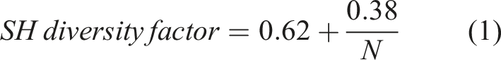
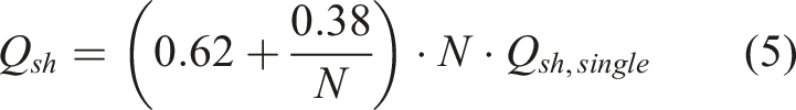
The SH diversity formulation presented in equation (1), where N is the number of dwellings, was originally developed for the combination of space and hot water needs in Danish district schemes. However, in CP1.2 it is considered applicable to SH demand alone on the assumption that there are heat losses to neighbouring properties that raise SH demand sufficiently to offset the absent DHW load. The accompanying recommendation is that further analysis using data from existing schemes is needed to develop a more robust diversity formulation.⁵

S H d i v e r s i t y f a c t o r = 0.62 + \frac{0.38}{N}

(1)

Estimating diversified DHW demands

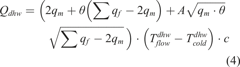
The Distributing Pipe Sizing section in the DS439 provides the method that is used in CP1.2 for the calculation of the design local flow rate, a requirement for pipe sizing,

q_{d} = 2 q_{m} + θ (\sum q_{f} - 2 q_{m}) + A \sqrt{q_{m} \cdot θ} \sqrt{\sum q_{f} - 2 q_{m}}

(2)

where q_m is the weighted mean water flow rate of all outlets connected to the distributing pipe, q_d is the design water flow rate for randomly used outlets connected to the distributing pipe, q_f is the sum of assumed water flow rates of randomly used connected outlets, A is the safety factor, and θ is the probability of draining q_m at times of peak demand. These factors are to be selected by the designer depending on the levels of service that are required. Although the method was originally developed for centrally generated water systems, CP1.2 justifies its use in HNs on the basis that flow rates on the secondary side of a HN are similar to those in systems with instantaneous hot water production.⁵

The diversity formulation in the DS439 pipe sizing equation has its roots in probability arguments. These arguments evolved into a formulation used for dimensioning district heating substations by 1997.¹⁹ The DS439 also provides a separate method for sizing heat exchangers, which has also been used by the UK HN industry.^6,8,12 This paper aims to inform the Code of Practice, which refers only to the pipe sizing methods in the DS439, so oversizing will be assessed in relation to that method only.

Space heat and hot water

Understanding how the behaviour of SH and DHW demand varies within a HN may hold immediate insights for design, as well as help comprehend the future implications of evolving DHW and SH needs. For example, the trend of increasing building insulation, which reduces SH demand, means that DHW demand may become increasingly dominant.²⁰ At present, DHW demand accounts for as little as 16% of the total demand of a dwelling.⁹ However, as domestic demands evolve, so too should technical guidance. As it stands, there is a distinct lack of literature that explores the SH and DHW demands within a HN. Studies of this kind would therefore greatly benefit the UK HN industry, in preparation for the rapid developments in the building stock and energy systems that are underway.

Research questions, data and methods

Research questions

This paper aims to aid the design of HNs in the UK by addressing the issues outlined above. Specifically, the study is guided by the following research questions.

• What temporal resolution of demand data is required to adequately capture peak demands?

• What is the empirical demand curve of the case study HN?

• What is the potential extent of oversizing in the case study HN?

• How does SH and DHW demand aggregate over dwellings and what are the implications for HN design?

To answer these questions, the paper analyses the individual and aggregate energy demands from a case study UK HN, measured by a novel data collection system at an unprecedentedly high-frequency. This is one of the first comprehensive analyses of data from such a system. Although this system was one of the first to support such analysis, similar levels of instrumentation are now commonplace. The resulting flow of data promises to transform the theory, design, and operation of HN systems in the coming decades.

Case study data

The case study is a single-building heat network, also known as a communal heat network (CHN), located in the Southeast of England. It serves approximately 150 apartments and was fully developed by 2018. A substantial portion of the dwellings had a design occupancy of 2 (1 bed), with the next largest group having a design occupancy of 4 occupants (2 bed). A small group had an occupancy of 6 and 3 occupants (3 bed and 2 bed respectively). The floor area of the dwellings had a range of 40 m² to 129 m², with a large proportion of dwellings having a floor area of 40-49 m². Although data were collected for most dwellings on the HN, after the data cleaning processes, demand profiles were produced for a group of 115 dwellings.

Heatweb Ltd. Developed a data collection system to gather data from hundreds of Heat Interface Units (HIUs) across multiple HNs, including from the case study that is examined in this paper. The system was built to aid effective monitoring and control of HNs and has been made available for academic research. This Internet-of-Things system consists of meters, sensors, and other hardware, supported by linked software programmes. The novelty of this system, relevant to this study, is that it enables data collection from a real HN at sampling times as low as one second. There are multiple sensors in each HIU in each apartment; those in the heat meter and others that are located elsewhere in the HIU. Both are connected via separate systems to a Raspberry Pi located in the building’s basement, through which the data are transmitted to a remote server. Connecting to this server allows data to be collected locally.

The analysis in this paper focusses on the week containing the coldest day in the monitored period. Figure 1 shows the daily mean external temperatures for that week. The lowest mean daily temperature was 2.5°C, with shorter spans of time where temperatures were as low as 1°C. Although external temperatures in the UK can be lower in extreme weather conditions, the monitored period is considered broadly representative of typical cold weather conditions.²¹

Figure 1.

Mean daily external temperatures of the case study HN over the selected cold period.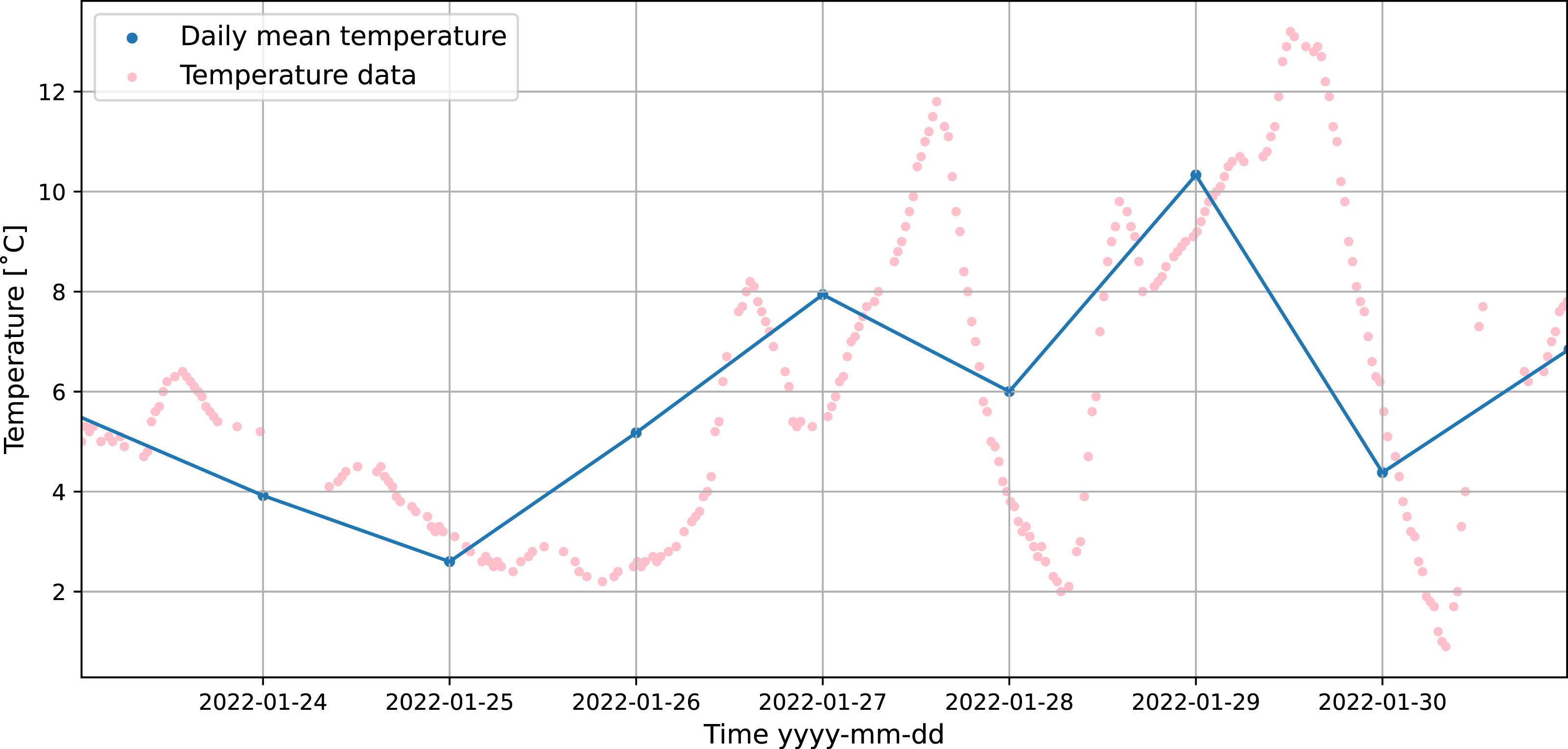

Estimating DHW demand and total demand

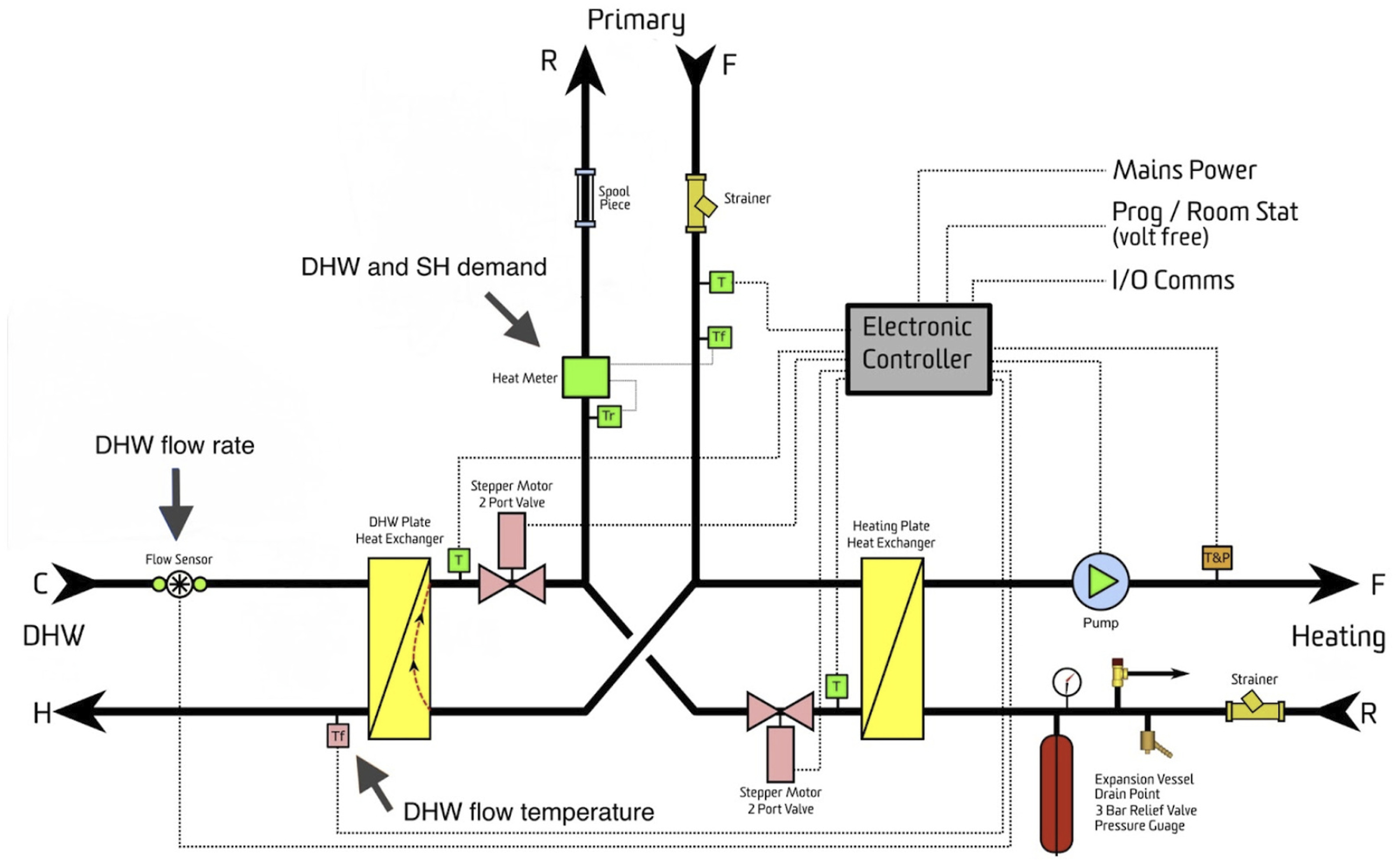
The richness of the available data allowed several methods for determining heat demand to be considered. Ideally, DHW demand and SH demand would have been determined separately; however, limitations in the dataset meant that SH demand could not be produced independently. Instead, the DHW demand, and the total demand, comprising both DHW and SH, were determined. The instantaneous total demand (kW) was determined using reliable heat meter data. The instantaneous DHW demand (kW) was estimated using the measured temperature and flow rate of hot water, and an assumed cold-water temperature. The sensor locations of the key measured variables are shown in the schematic in Figure 2. Comparing the metered total demand to the estimated DHW demand allowed partial disaggregation of the roles of SH and DHW in driving the aggregate peak. The selected methods for determining demands produced results with the lowest uncertainties while ensuring that demand profiles could be produced for a large enough number of dwellings such that the diversity effect could be investigated effectively.¹⁴

Figure 2.

Schematic of the HIU showing the sensor locations of the key measured variables²².

The temperature of incoming cold water is a relatively stable figure roughly equal to the annual mean outside air temperature in the UK, which is approximately 10°C.²³ Therefore, the cold water temperature in the DHW demand calculation was taken to be 10°C. Figure 3 shows that the minimum DHW flow temperature for the dwelling group is approximately 10°C, which supports this assumption.

Figure 3.

DHW flow temperatures for the group of dwellings.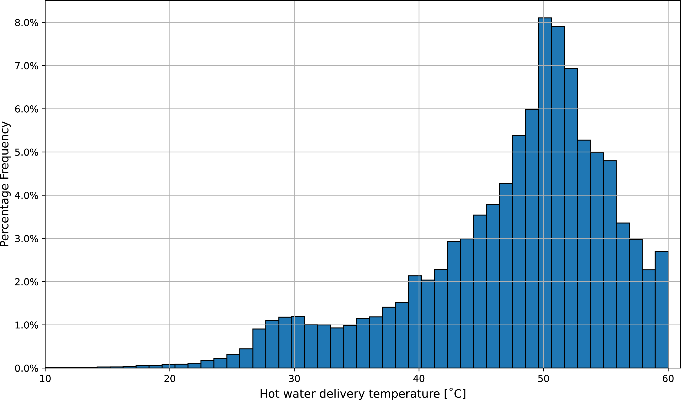

Since the DHW flow rate and temperature data collection were event-based, meaning a data point would only be recorded if it differed from the previous one, the resulting time-series was forward-filled to produce a series with uniform time intervals. The heat meter data, used for determining the total demand, was collected at 5-min intervals. Often, the last flow rate data point of a DHW demand event, which would be 0 l/m, was missing. If this missing data were left unaddressed when forward-filling, it would lead to DHW demand events appearing to end in a low-level leak. To address this issue, an algorithm was developed to identify and fill in the missing data points. To ensure successful removal, all demand profiles were then inspected visually. Additionally, spurious readings with unknown causes were found in both the metered total demand and the estimated DHW demand profiles. These occurrences were rare enough that the affected dwellings could be removed entirely without significantly compromising subsequent analysis.

Aggregating demands

In order to represent the energy demands across the pipe network, aggregate demands of varying dwelling-group size were considered. As previously noted, the sampling time of the individual energy demands can measurably impact the aggregate demands it produces, and therefore the role of sampling time must be carefully investigated. With this end in mind, the individual dwelling demand profiles were resampled by averaging over increasing time intervals, and each set used to create aggregate demand profiles for dwelling-groups of varying size. The intended result is a family of demand profiles for each point along the network, each of which shows the impact of sampling time. Therefore, altogether, the effect of two kinds of aggregation is shown in the results of this paper: aggregation over the number of dwellings and aggregation over time.

Aggregating over time, or resampling, means to average the data points over increasingly large time steps. Note that the term ‘sampling time’ is used to refer to both the time interval at which the raw data are collected and the larger time intervals over which the raw data are averaged. The time intervals used for DHW demand were 1, 5, 10, and 30 s; 1, 5, 10, and 30 min; and 1 h. The sampling time of the raw DHW demand data was 1 s. For the metered total demand, time intervals below 5 min could not be used because the raw data were collected at 5-min intervals. Consequently, for the total demand, time intervals of 5, 10 and 30 min; and 1 h were used.

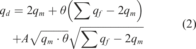
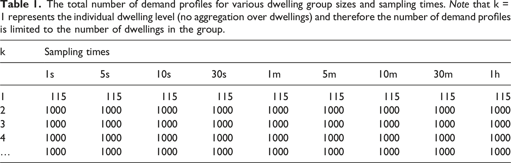
When creating an aggregate demand profile for any number of dwellings, k, there are many unique combinations of k dwellings that can be selected from the total pool of N dwellings. The total number of unique combinations, T, for a k sized pool of N dwellings is given in equation (3).

T = \frac{N!}{k! (N - k)!}

(3)

Equation (3) shows that T can get extremely large. For example, where N = 81, k = 5 results in T = 2.56 × 10⁷ and k = 35 results in T = 1.02 × 10²³. To avoid unreasonably large computational times, the maximum number of dwelling combinations was therefore limited to 1,000. It is important to note that where the value of k is close to that of N, the resulting aggregate profiles are likely to be made up of more of the same individual dwellings, thus becoming more and more similar. Table 1 summarises the total number of profiles created at each sampling time for each level of aggregation over the number of dwellings. Note that individual dwelling demand profiles are considered to be a group of one dwelling, labelled the ‘k = 1’ group. The ‘k = 2, 3, 4, …’ groups represent the aggregate of 2, 3, 4, … dwellings.

Table 1.

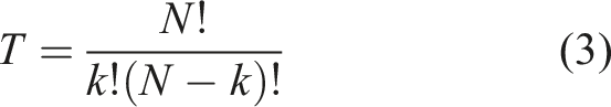
The total number of demand profiles for various dwelling group sizes and sampling times. Note that k = 1 represents the individual dwelling level (no aggregation over dwellings) and therefore the number of demand profiles is limited to the number of dwellings in the group.

k	Sampling times
	1s	5s	10s	30s	1m	5m	10m	30m	1h
1	115	115	115	115	115	115	115	115	115
2	1000	1000	1000	1000	1000	1000	1000	1000	1000
3	1000	1000	1000	1000	1000	1000	1000	1000	1000
4	1000	1000	1000	1000	1000	1000	1000	1000	1000
…	1000	1000	1000	1000	1000	1000	1000	1000	1000

Evaluating oversizing

Oversizing was evaluated by developing two empirical demand curves, a mean-peak curve and a maximum-peak curve, and by comparing them to a design curve. The design curve was determined using the methods recommended in CP1.2 and guided by the worked example in its Annex D.⁵ The mean-peak demand of the case study was compared to the design demands to assess the possible extent of oversizing, assuming that the HN was built based on the guidance in CP1.2, and the maximum-peak curve is presented to illustrate the extent to which peak demands can increase under the least favourable diversity conditions.

Empirical demand metrics

Both empirical demand curves consist of a demand value for the individual level (k = 1 dwelling) and for every level of aggregation (k = 2, 3, 4, …, 91 dwellings). An upper limit of k = 91 was imposed to prevent repeated sampling of the same combination of dwellings. To illustrate the calculation of the mean-peak and maximum-peak, consider their calculation for the individual dwelling level. The mean-peak is obtained by averaging the peak demands of the dwelling group, giving a single value to represent the entire group. Since there are 115 individual dwelling demand profiles (one for each of the 115 dwellings in the group), the resulting mean-peak is the average of 115 peak demand values (as shown in Table 1, where k = 1). On the other hand, the maximum-peak demand represents the peak demand of the dwelling with the highest peak demand in the group, and therefore only reflects that particular dwelling. This distinction is further illustrated in Figure 4.

Figure 4.

Illustration of the mean-peak and maximum-peak calculations at the individual dwelling level, using five dwellings as an example.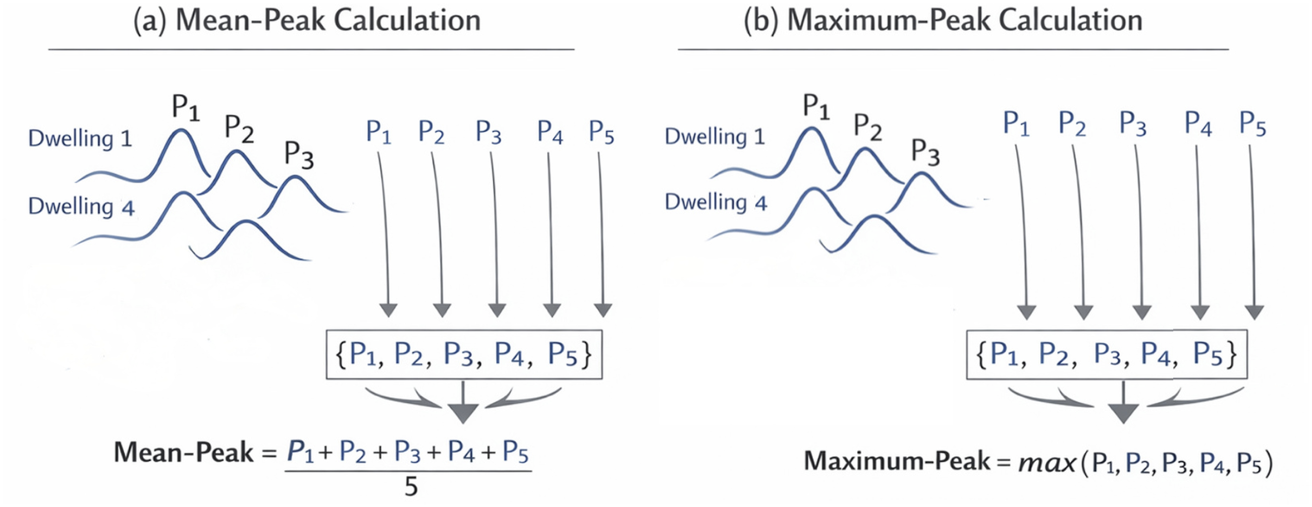

At aggregate levels of 2, 3, 4, …, 91 dwellings, the maximum-peak metric represents the peak of the aggregate demand of the combination of dwellings (1000 combinations in total, as shown in Table 1 for k > 1) that creates the largest peak (i.e. where there is the least diversity). In contrast, the mean-peak is determined by averaging the aggregate peak demands of the 1000 combinations of dwellings. Consequently, at aggregate levels, the maximum-peak is the peak that results from the least diversity, while the mean-peak represents an average of the range of possible diversities for this sample of dwellings.

In practical terms, the maximum-peak at the individual level can only be used to indicate oversizing in the pipe directly connected to the dwelling with the highest peak demand. This metric therefore ignores the oversizing of pipes connected directly to all other dwellings. On the other hand, the mean-peak metric at the individual level can be used to indicate the average amount of oversizing across all pipes directly connected to a dwelling.

Design demand estimates

The guidance provided in CP1.2 gives DHW diversity in terms of flow rates and SH diversity in terms of a diversity factor. Both equations have been adapted here to be in terms of demand, as shown in equations (4) and (5), and to be used to produce a design demand curve. For DHW demand, the diversified flow rate is used with a temperature delta in the DHW circuit to determine the demand of a group of N dwellings. For the SH demand, the diversity factor is used with an assumed single dwelling SH demand to give aggregate SH demands. The values used are provided in Table 2. CP1.2 states that all the given values that make up the diversity calculation are considered suitable for most applications. For more unique cases, detailed calculations and modelling are recommended.

Q_{d h w} = (2 q_{m} + θ ({\sum q}_{f} - 2 q_{m}) + A \sqrt{q_{m} \cdot θ} \sqrt{{\sum q}_{f} - 2 q_{m}}) \cdot (T_{f l o w}^{d h w} - T_{c o l d}^{d h w}) \cdot c

(4)

Q_{s h} = (0.62 + \frac{0.38}{N}) \cdot N \cdot Q_{s h, s i n g l e}

(5)

Table 2.

The variables used in determining design demand.

Demand	Variable	Notation	Value	Source
DHW	Weighted mean water flow rate (l/s)	$q_{m}$	0.1	Objective 3.2 and annex D in CP1.2.⁵
	Assumed water flow rate of randomly used outlets (l/s)	$q_{f}$	0.2-0.35	Table 9, Section 3.9.15 in CP1.2 where the minimum is 0.15 l/s, however, here it is adjusted to 0.2 l/s in order to keep the square-root component positive.⁵
	Safety factor	$A$	3.1	Objective 3.2 states that the DS439 gives this value for a residential building.⁵
	Probability of draining $q_{m}$ at times of peak demand	$θ$	0.015	Objective 3.2 states that the DS439 gives this value for a residential building.⁵
	Number of dwellings	$N$	1-91	—
	Sum of assumed water flow rates (l/s)	${\sum q}_{f}$	Equal to $N \times q_{f}$	—
	Flow temperature (˚C)	$T_{f l o w}^{d h w}$	45	Lower bound given in HIU specification.²² Measurements reflect this value (see Figure 3).
	Cold water temperature (˚C)	$T_{c o l d}^{d h w}$	10	Based on findings by the energy savings Trust.²³
	Specific heat capacity (kJ/kg˚C)	$c$	4.182	Established empirical value.²⁴
SH	Number of dwellings	$N$	1-91
SH	SH demand of single dwelling (kW)	$Q_{s h, s i n g l e}$	2-3	Table 11, Annex D in CP1.2.⁵

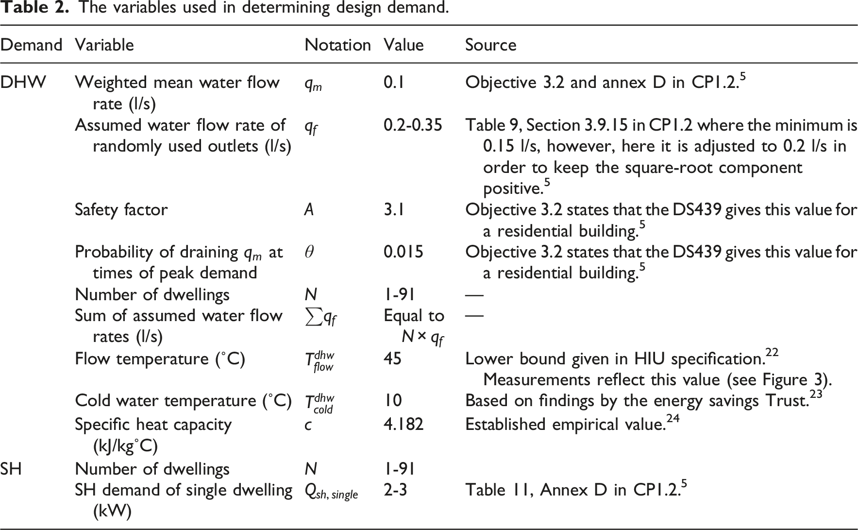
The measured flow rates of the case study tended to have a value of 0.1 l/s, with the maximum recorded flow rate being 0.26 l/s. The assumed flow rate of a randomly used outlet, q_f, having a range of 0.2–0.35 l/s, could therefore be argued to be too high.

Results

Case study heat demands

This section aims to demonstrate how the heat demands of the case study align with expected behaviours, while also highlighting its idiosyncrasies. By providing this grounding, readers can contextualise the results of the subsequent sections and be able to apply them to similar HNs. Figure 5 illustrates the aggregate DHW demand and aggregate total demand of the dwelling group over the selected cold period. The total demand appears to be aligned with the external temperature, as evident when comparing the coldest day, the 25^th, to the warmest day, the 29^th, showing significantly higher demands on the colder day. This is expected because SH demands, which make up part of the total demand are strongly coupled to the external environment. The total demand may also include a contribution from the ‘keep-hot’ function which requires that the primary circuit in the HIUs be kept warm, ready for a DHW draw. The demand associated with this function would only be captured by the metered data because the meter is located on the primary side of the HIU (while the sensors are located on the secondary side). Consequently, it would only be evident in the total demand profile and not in the DHW demand profile.

Figure 5.

Aggregate DHW and total demand for the selected cold period at a sampling time of 5 min.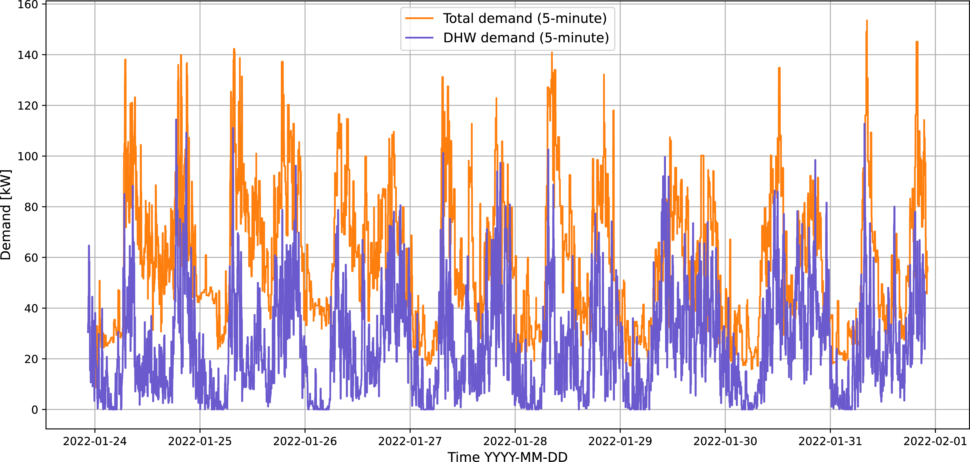

Figure 6 illustrates the mean hourly 24-h DHW and total demand profiles for the group of dwellings during the selected cold period. Both profiles demonstrate the typical demand peaks, occurring in the morning and evening, as observed in previous studies.^25,26 Notably, the comparison of the two profiles reveals that the proportion of DHW in the total demand is approximately 50%. This suggests that, on an annual basis, including the off-heating season when SH demand is absent, the proportion of DHW demand in the total demand, for this particular development, would exceed 50%. Other studies have reported that DHW demand can account for as little as 16% of the annual total energy demand, or as much as 40–50% in energy-efficient homes.^9,27 This suggests that the proportion of DHW demand in this dwelling sample is high. This could be because of low SH demand, which may be attributed to several factors. Firstly, the building, being a newbuild, is likely to have higher levels of insulation compared to older dwellings in the wider UK stock. Secondly, the dwelling sample consists solely of apartments, which have fewer external walls, contributing to a lower SH demand without affecting DHW demands.

Figure 6.

Mean hourly 24-h DHW and total demand profiles for the group of dwellings over the selected cold period.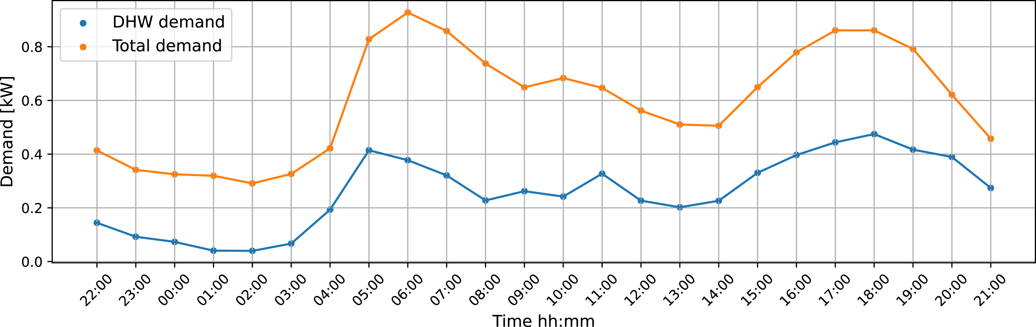

The impact of sampling time on peak demands

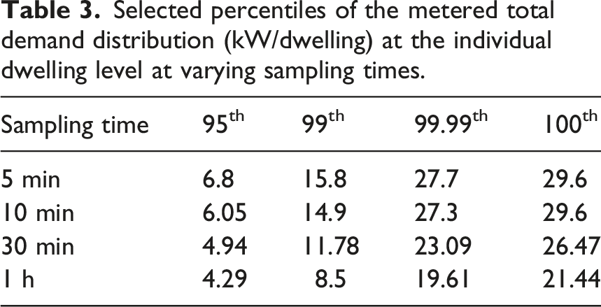
In order to recommend a sampling time for measuring demand data in existing networks to create an evidence base useful for designing new networks, the impact of varying sampling size on individual dwelling demands was investigated. Figure 7 shows the distribution of metered total demand for individual dwellings at sampling times of 5, 10, 30, and 60 min. Table 3 summarises the percentiles of the total demand distributions. Notably, the maximum demand (the 100^th percentile) for both 5-min and 10-min sampling times is precisely equal at 29.6 kW. However, as sampling times exceed 10 min, the maximum demand gradually decreases. At 30 min, it is 26.47 kW, while at one hour, it further reduces to 21.44 kW.

Figure 7.

The metered total demand distribution at the individual dwelling level showing the impact of increasing sampling time. Top-left: 5-min; top-right: 10-min; bottom-left: 30-min; bottom-right: 1-h.

Table 3.

Selected percentiles of the metered total demand distribution (kW/dwelling) at the individual dwelling level at varying sampling times.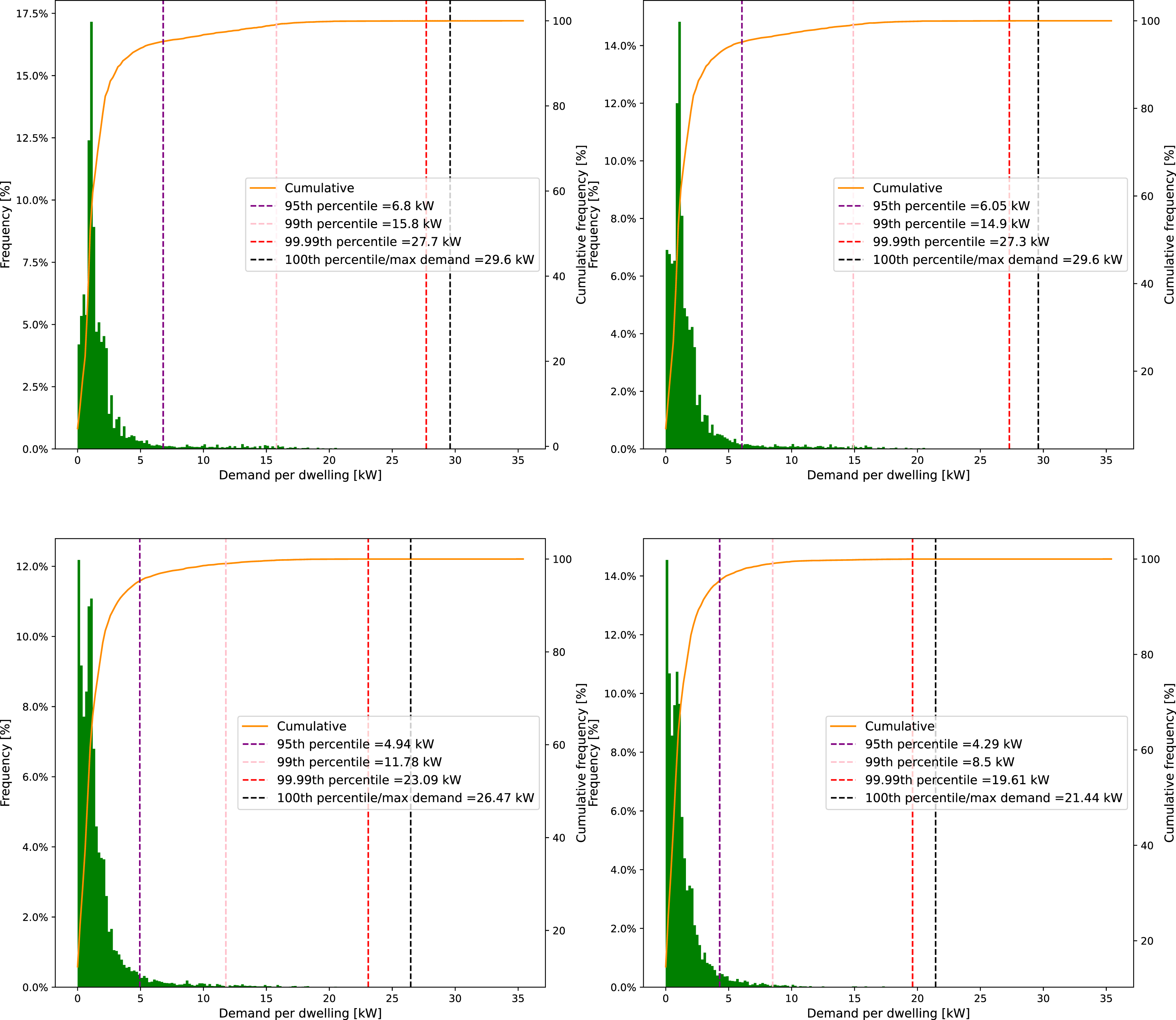

Sampling time	95^th	99^th	99.99^th	100^th
5 min	6.8	15.8	27.7	29.6
10 min	6.05	14.9	27.3	29.6
30 min	4.94	11.78	23.09	26.47
1 h	4.29	8.5	19.61	21.44

The 100^th percentile of the total demand distribution, being exactly equal at a sampling time of 5 and 10 min suggests that the 100^th percentile for sampling times lower than 5 min would also be the same. This implies that a sampling time of 10 min is sufficient to fully capture the true peak demand in the case study and may serve as a useful starting point for defining an adequate monitoring resolution for data-informed network sizing more broadly. Confidence intervals were produced using a bootstrapping method that involved producing 5000 samples of dwellings with replacement. The confidence interval for the 100^th percentile of total demand at a 10-min resolution is 25.8 kW to 29.6 kW. This suggests that variability in the dwelling sample is likely to result in a peak demand within this range. At a sampling time of 5 min, the confidence intervals remain unchanged. The non-change in confidence intervals shows that the similarity between peak demands at 5- and 10-min resolutions is not sensitive to which dwellings are sampled. This reinforces the conclusion that a 10-min resolution is sufficient for peak demand estimation.

Note that each data point that makes up the metered total demand distribution at the base sampling time of 5 min (shown in the top-left distribution of Figure 7) corresponds to either SH demand or DHW demand, never a combination of both, as it is unprocessed data. This is due to the DHW-priority function in the HIUs which gives DHW draw-offs priority over any SH demand that may be present at the same time. As the unprocessed data are resampled, however, because of the averaging over adjacent data points, the demand distribution will increasingly contain data points that represent a mix of both DHW and SH demands.

In the DHW demand distributions, shown in Figures 8–10, there is a mode at ∼15 kW for sampling times below 5 min. This suggests that the majority of the dwellings’ hot water demands are around 15 kW and tend not to last more than 5 min. Comparing the distributions of the total and DHW demands at the 5-min sampling time (top-left in Figure 7 and top-right in Figure 9 respectively) suggests that SH demands tend to be approximately 2 kW. This is evident because the total demand distribution has a mode at ∼2 kW, which is absent from the DHW demand distribution. This suggests that demands of around 2 kW are primarily SH demands, which support assumptions in CP1.2.⁵

Figure 8.

DHW demand distribution at the individual dwelling level showing the impact of increasing sampling time. Top-left: 1-s; top-right: 5-s; bottom-left: 10-s; bottom-right: 30-s.

Figure 9.

DHW demand distribution at the individual dwelling level showing the impact of increasing sampling time. Top-left: 60-s; top-right: 5-min; bottom-left: 10-min; bottom-right: 30-min.

Figure 10.

DHW demand distribution at the individual dwelling level at a sampling time of 1 h.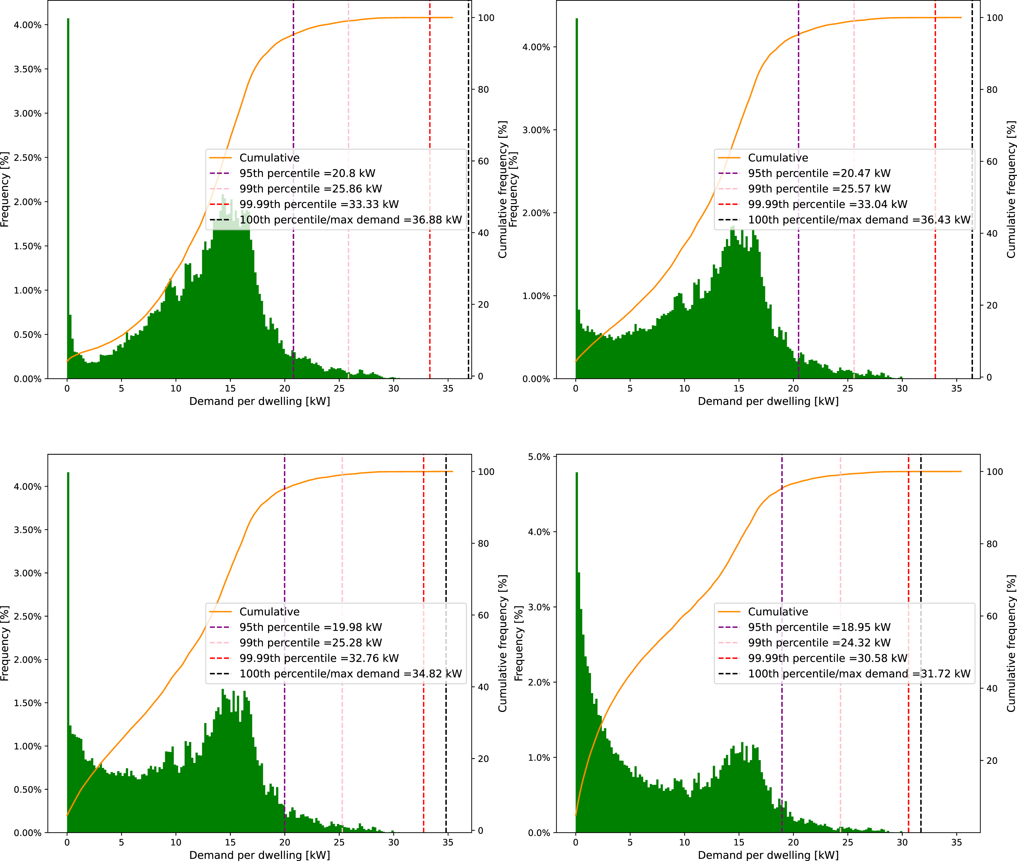

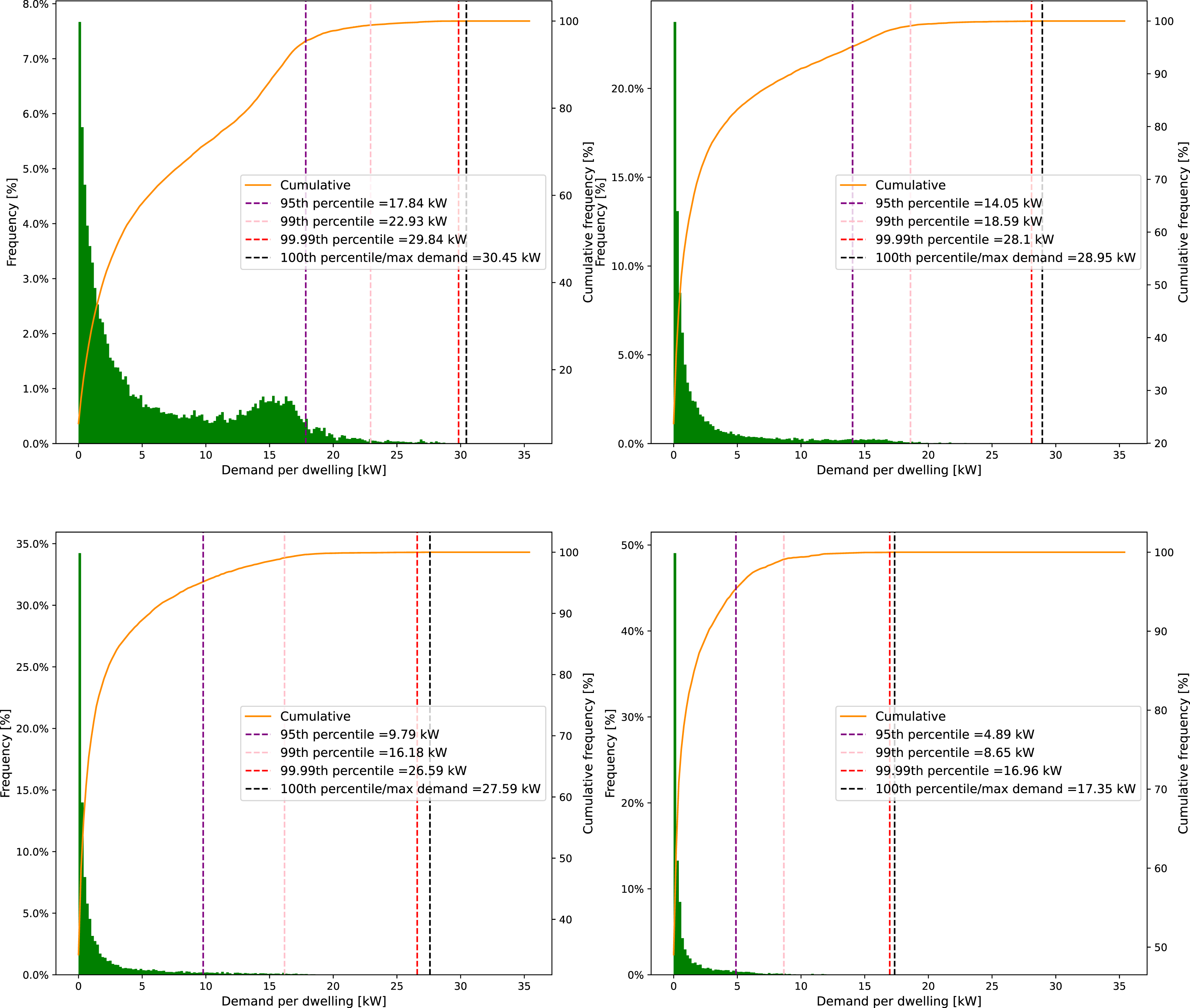
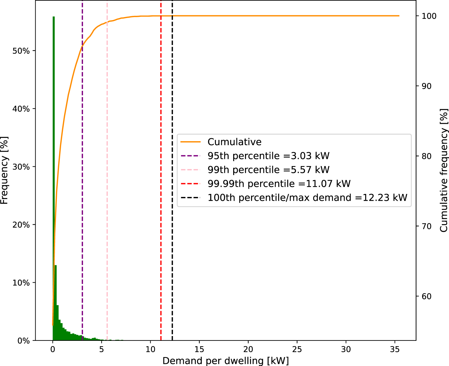
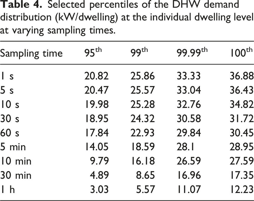
If the peak total demand (the 100^th percentile) at 5- and 10-min sampling times are equal, it can be assumed that the peak demand will remain the same at a 1-s sampling time. The measured peak total demand may arise from either DHW draw or a SH requirement. If the peak is attributable to DHW, the metered total demand can be directly compared with the DHW estimates. Comparing the total demand peak of 29.6 kW (see Table 3) to the DHW demand peak of 36.88 kW (see Table 4) shows that there is a discrepancy in the metered total demand and the estimated DHW demand. This is likely due to the cold water temperature assumption of 10°C being lower than the real value for at least some of the time. This is expected as 10°C is the minimum temperature reported by the Energy Savings Trust²³ which showed the full range could be from 10°C to 22°C, with the mode being between 14°C and 16°C. Since this only leads to a discrepancy in the total and DHW demands at sampling intervals shorter than 10 min, and all subsequent analyses use a 10-min sampling time, its impact on the results that follow is considered negligible.

Table 4.

Selected percentiles of the DHW demand distribution (kW/dwelling) at the individual dwelling level at varying sampling times.

Sampling time	95^th	99^th	99.99^th	100^th
1 s	20.82	25.86	33.33	36.88
5 s	20.47	25.57	33.04	36.43
10 s	19.98	25.28	32.76	34.82
30 s	18.95	24.32	30.58	31.72
60 s	17.84	22.93	29.84	30.45
5 min	14.05	18.59	28.1	28.95
10 min	9.79	16.18	26.59	27.59
30 min	4.89	8.65	16.96	17.35
1 h	3.03	5.57	11.07	12.23

Empirical demand curves and oversizing

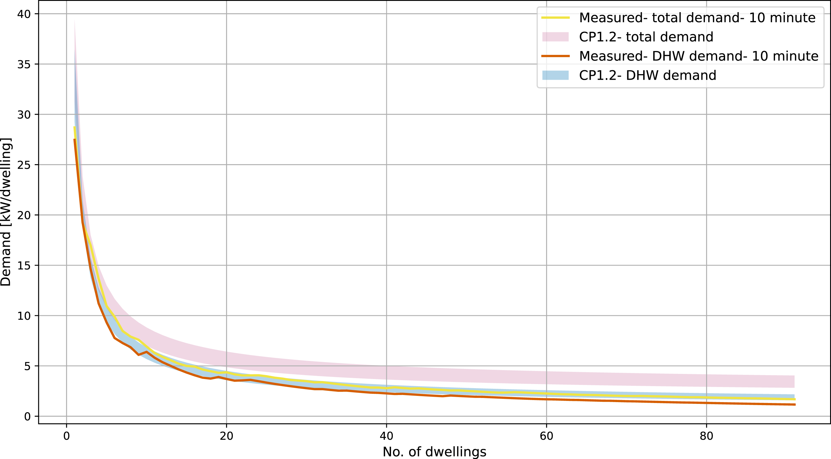
This section compares the measured demand curves against the design demand curve. The maximum-peak curve represents a useful limit showing the peak demand of the dwelling-combination with the lowest diversity at each level of aggregation. The mean-peak is a representation of the full range of possible dwelling-combinations and their associated diversities. The two curves can be compared to indicate how the variability of peak demands is affected as aggregation level increases. The mean-peak curve is used to estimate the potential extent of oversizing in the case study HN, while the maximum-peak is used to assess whether oversizing persists under low-diversity conditions.

Comparing Figures 11 and 12 shows that as the number of dwellings increases, the difference between the mean-peak and maximum-peak diminishes. This is because the spread in peak demands decreases with increasing number of dwellings, leading to similar mean and maximum values. Consequently, the peak demands at higher levels of aggregation can be viewed as a more stable figure. The decrease in spread may also be due to the fact that as the level of aggregation approaches the dwelling group size, the aggregate profiles are made up of more and more of the same dwellings. As a result, the aggregate demands of distinct dwelling combinations become less distinguishable for a given level of aggregation. Conversely, for lower levels of aggregation, the aggregate demand profiles are likely to be made up of more distinct sets of dwellings.

Figure 11.

Total and DHW design demands and their measured mean-peak counterparts.

Figure 12.

Total and DHW design demands and their measured maximum-peak counterparts.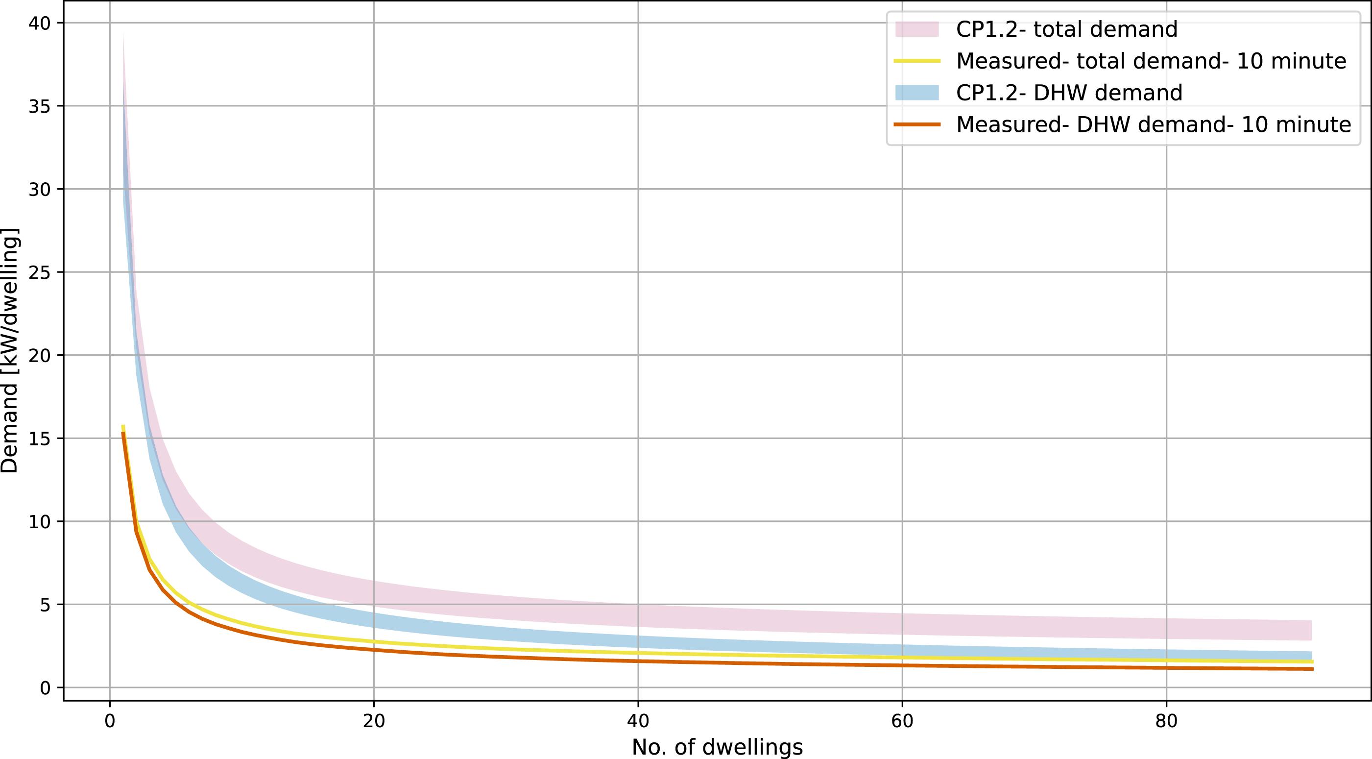

Figure 11 demonstrates that the mean-peak total and DHW demand at the individual dwelling level are each near 15 kW, with an approximate difference of ∼0.5 kW that persists across all levels of aggregation. This may be a useful rule of thumb for designers. Figure 11 also shows that both DHW and total demands may have been significantly overestimated, particularly at lower levels of aggregation. Table 5 gives the percentage overestimation for 5, 15 and 35 dwellings showing that that demands are overestimated by 52% at a minimum across these levels.

Table 5.

Comparison of design demand and mean-peak demand.

Demand	Number of dwellings	Design capacity (kW/dwelling)	Measured value (kW/dwelling)	Overestimation (%)
DHW	5	9.35 – 10.91	5.1	83 – 114
	15	4.32 – 5.32	2.63	64 – 102
	35	2.57 –3.34	1.69	52 – 98
Total	5	10.74 - 13.0	5.69	89 – 128
	15	5.61 – 7.26	3.15	78 – 130
	35	3.83 – 5.23	2.18	76 – 140

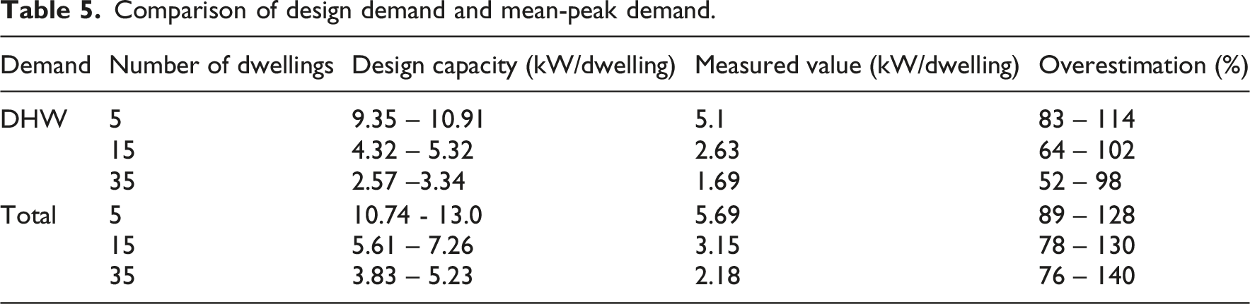
Figure 12 illustrates that when maximum-peak demands are considered, the design demands still significantly overestimate both total and DHW demands, especially at very low levels of aggregation. Note that in systems where SH is not suppressed during DHW draws, the maximum-peak demands may be higher due to both demands acting together. However, the curves also suggest that for the middle levels of aggregation (below approximately 40 dwellings), the measured DHW demand falls within its estimated range. This chart raises questions about the necessity of the SH addition in the design estimates, as it shows the total measured demand is within, or close to within range, of the DHW design estimates alone, across all but the very lowest levels of aggregation.

Discussion

The aim of this paper was to investigate the concerns regarding the current HN sizing guidance, for which the energy demands of a case study were analysed in line with the stated research questions. The analysis indicated significant potential oversizing within the case study, reinforcing the concerns about DS439-based sizing methods. The key findings are summarised below.

• A sampling time of 10 min was found to sufficiently capture peak demands in the case study and may serve as a useful starting point for defining data resolution recommendations for informing network sizing more broadly.

• Empirical total demand and DHW demand curves were produced that may serve as a reference of interest for designers of similar networks, and which can be used as part of a wider evidence base to guide UK HN design.

• Oversizing of the case study HN appears to be significant and in the range of 52%-140%.

• The measured total demand was found to be consistently ∼0.5 kW above the DHW demand across all levels of aggregation.

• The close match between the total demand curve and the DHW curve raises questions about the necessity of the SH component in the design methods.

CP1.2 recommends using data measured at one-minute intervals to develop empirical demand curves for HN sizing. In contrast to this, the work presented in this paper found that a 10-min sampling time is sufficient for measuring the peak demands of the case study. This sampling interval may be sufficient for capturing the peak demands of other HNs serving a similar dwelling-stock and occupancy, with comparable SH and DHW system configurations, provided monitoring is conducted for a sufficiently long period during the heating season. It is important to note that this benchmark value may vary for HNs that significantly differ from the case study. For example, where there is dwelling-level hot water storage, which has a flattening effect on demand, it is expected that a coarser sampling time would sufficiently capture peak demands.

There are several reasons why the methods in CP1.2 may overestimate peak demands, including assumptions of system flow rates and temperatures no longer reflecting current conditions. Numerous studies have reported discrepancies between measured DHW flow rates and those recommended by various European design standards, including the DS439.^9–11 These studies attribute the mismatch to substantial changes in DHW system design since the standards were developed, and to evolving occupant consumption behaviour. Furthermore, the Energy Savings Trust²³ found that measured DHW temperatures are lower than those assumed in commonly used standards. Together, these factors may contribute to the resultant oversizing. Future work could involve quantifying the contribution of each of these factors to the resultant oversizing.

CP1.2 recommends calculating SH and DHW diversity for each pipe section independently and then combining the results to obtain a total flow rate. However, comparing the measured demand curves to the design estimates raises questions about whether the SH addition is necessary. The metered total demands fall within the range of the DHW design estimates alone, suggesting that the SH component in the methods may not be required. Removing it from the design methods may be a reasonable short-term measure to mitigate oversizing; however, a more prudent and robust solution is the development of a comprehensive evidence base of empirical demand curves for different types of HNs, such that designers will no longer have to rely on the outdated, probability-based methods.

It is common practice to intentionally oversize systems to ensure all demands, including those arising under unlikely conditions, are met. This is not unreasonable, given that maintaining occupant comfort across all possible scenarios is a primary design objective. However, considering the rarity of such occurrences, the benefits of oversizing may not justify the associated penalties: greater thermal losses, higher capital expenditure, and increased running costs. This is why the demands presented in this work, those representative of typical peak conditions, are presented for guiding system design. Even where designers choose to apply an overestimation factor to peak demands, they may still benefit from knowing the true values under non-exceptional conditions. The mean-peak and maximum-peak demands presented in this paper reflect realistic diversity scenarios arising from different possible dwelling combinations under the monitored conditions. There may be circumstances in which conditions depart from those in this work. For example, external temperatures falling below 0°C may alter energy demand patterns. Future work could model or empirically assess such extreme scenarios to investigate how the resulting demand curves differ. Nevertheless, the question of whether systems should be sized to these extreme conditions remains open, and in practice will be governed by the level of risk that designers are willing to accept liability for.

Prior to this study, only two empirical investigations into diversity in UK HNs existed. The first developed empirical demand curves but relied on data from homes heated by means other than a HN.¹³ The present work improves this evidence by providing an empirical demand curve using a real HN. The second examined oversizing relative to the heat exchanger sizing methods specified in the DS439.^6,12 The present work compliments this by confirming oversizing in relation to the pipe sizing methods. The heat exchanger sizing methods and pipe sizing methods, both of which are commonly used to size UK HNs, have therefore been shown to carry significant potential for oversizing. Beyond these two studies, there is a notable lack of research drawing on real HN data to evaluate sizing methods in the UK context. With both key sizing methods demonstrated to substantially overestimate capacities, and so few related studies to draw on, there is a clear need for data-driven sizing resources to support designers. The work presented in this paper serves as a foundational starting point for meeting that need. CHNs are those that serve single buildings and they represent a significant share of existing, and likely future, HNs.²⁸ Since the findings presented here are grounded in data from a real CHN, they are likely to be applicable to many future UK HN developments. Nonetheless, building a robust evidence base comprising a family of empirical demand curves alongside necessary accompanying investigations such as those presented in this paper is paramount to ensuring the effective design of the full range of future UK HNs.

Limitations

A key limitation of this work concerns the distinction between real and aggregate demand. The study assumes that aggregate demand accurately represents the real demand at a specific point within the distribution system. For instance, it assumes that the aggregate demand of ten dwellings is equivalent to the demand measured directly within a pipe section serving those ten dwellings. However, this assumption has not been empirically verified. Confirming its validity would require measurement studies that capture demand data at multiple locations throughout the distribution network. Real demand profiles are likely to be flatter than aggregate profiles due to mixing effects and variations in fluid velocity within the pipework, meaning that aggregate data may overstate the sharpness of real peaks.

Conclusions

This study is one of the first to use measured, high-resolution data to investigate heat demand and its diversity across dwellings. As part of this, empirical demand curves were developed, and several practical recommendations emerged for designing new networks. A 10-min sampling interval was recommended for measuring demand in homes on existing HNs to inform the design of comparable schemes. The total demand was empirically shown to be consistently ∼0.5 kW higher than DHW demand across all levels of aggregation. An empirical demand curve was compared with a design curve, raising questions about the necessity of the SH addition in current design guidance. In light of the oversizing evaluation in this work, the case study network was shown to be oversized by between 52% and 140%.

The findings indicate potential for significant capital and operational expenditure savings on future HNs by reducing oversizing. It is likely that the potential oversizing seen in the case study is not unique, given that all existing networks are likely to have used the same design estimation methods. Future work, based on examining the extent of oversizing in other UK HNs, would help to indicate the scale and severity of the problem. This would bring attention to a significant issue in the fast-growing HN industry before it becomes systemically proliferated.

The data system used in this work was one of the first of its kind, as were the methods and results presented. However, as such data monitoring systems become increasingly common due to their growing value for operational management, an increasing flow of similarly high-resolution data can be expected. This new data stream should be used to undertake studies similar to that presented in this paper for HNs of varying size, topology, and consumer composition. Such work would, for instance, enable the development of a family of demand curves to inform UK HN design more broadly. The desired outcome is a robust evidence base that the design community could use to inform new designs. A new or existing working group could be tasked with developing and costing a plan to create this evidence base, including identifying any requirements for government funding, such as for building and maintaining the underlying datasets.

Supplemental material

Supplemental material - Informing efficient heat network design: Peak demand, diversity and network sizing

Supplemental material for Informing efficient heat network design: Peak demand, diversity and network sizing by Niki Sahabandu, Jenny Crawley, Robert J. Lowe in Building Services Engineering Research & Technology.

Footnotes

Acknowledgements

The authors would like to express their gratitude to Richard Hanson-Graville for their generosity in providing access to data collected by the Heatweb system. They also thank George Bennett for being part of the supervisory team that guided the PhD work on which this paper is based, and Paul Woods for providing valuable and industry-relevant feedback on the PhD. The authors would also like to thank Olly Smith for their helpful guidance on a key statistical component of the paper.

ORCID iDs

Niki Sahabandu

Jenny Crawley

Funding

The authors disclose receipt of the following financial support for the research, authorship, and/or publication of this article: This research was made possible by the Engineering and Physical Sciences Research Council (EPSRC) support for the London-Loughborough Centre for Doctoral Research in Energy Demand (LoLo) (grant numbers EP/L01517X/1 and EP/H009612/1).

Declaration of conflicting interests

The authors declared no potential conflicts of interest with respect to the research, authorship, and/or publication of this article.

Supplemental material

Supplemental material for this article is available online.

References

Committee on Climate Change . The sixth carbon budget: the UK’s path to net zero. Report of the Committee on Climate Change 2020. https://www.theccc.org.uk/wp-content/uploads/2020/12/The-Sixth-Carbon-Budget-The-UKs-path-to-Net-Zero.pdf. (accessed 1 December 2025).

Department for Energy Security and Net Zero . Carbon budget and growth delivery plan. Report of the Department for Energy Security and Net Zero 2025. https://assets.publishing.service.gov.uk/media/6901d0c2a6048928d3fc2b55/carbon-budget-and-growth-delivery-plan-report.pdf. (accessed 1 December 2025).

United nations framework convention on climate change. Paris agreement. 2015. https://unfccc.int/sites/default/files/english_paris_agreement.pdf. (accessed 1 December 2025).

Chartered Institute for Building Services Engineers, Association for Decentralised Energy . Heat networks: code of practice for the UK. 1st ed. Chartered Institute for Building Services Engineers publications, 2014.

Chartered Institute for Building Services Engineers, Association for Decentralised Energy . Heat networks: code of practice for the UK. 2nd ed. Chartered Institute for Building Services Engineers publications, 2020.

Smith

. On a mission: using data to optimise heat networks. 2016. https://www.cibsejournal.com/technical/on-a-mission-using-data-to-optimise-heat-networks/. (accessed 1 December 2025).

Weissmann

Hong

Graubner

. Analysis of heating load diversity in German residential districts and implications for the application in district heating systems. Energy Build 2017; 139: 302–313. https://doi.org/10.1016/j.enbuild.2016.12.096

Dansk Standard . DS439. Code of practice for domestic water supply installations. Dansk Standard, 2009.

Fuentes

Arce

Salom

. A review of domestic hot water consumption profiles for application in systems and buildings energy performance analysis. Renew Sustain Energ Rev 2018; 81: 1530–1547. https://doi.org/10.1016/j.rser.2017.05.229

10.

Jack

Patidar

Wickramasinghe

. A proposed new UK framework for the sizing of domestic hot and cold water systems for medium-large scale residential buildings. 2017; https://doi.org/10.13140/RG.2.2.15157.99045

11.

Koiv

Toode

. Trends in domestic hot water consumption. Proc Estonian Acad Sci Eng 2006; 12: 72–80. https://doi.org/10.3176/eng.2006.1.06

12.

Open Data Institute . Case study: Guru systems improving energy efficiency through open data. , 2016.Open Data Institute.

13.

Wang

Crawley

Francis

GNL

, et al. Sizing of district heating systems based on smart meter data: quantifying the aggregated domestic energy demand and demand diversity in the UK. Energy 2020; 193: 116780. https://doi.org/10.1016/j.energy.2019.116780

14.

Sahabandu

CN.

Informing heat network design: a study of demand diversity and domestic hot water storage using high resolution measured data. University College London, 2025. PhD Thesis. Available from: https://discovery.ucl.ac.uk/id/eprint/10206285/

15.

Happle

Fonseca

Schlueter

. Impacts of diversity in commercial building occupancy profiles on district energy demand and supply. Appl Energy 2020; 277: 115594. https://doi.org/10.1016/j.apenergy.2020.115594

16.

McKenna

Hofmann

Merkel

, et al. Analysing socioeconomic diversity and scaling effects on residential electricity load profiles in the context of low carbon technology uptake. Energy Policy 2016; 97: 13–26. https://doi.org/10.1016/j.enpol.2016.06.042

17.

Guan

Nord

Chen

. Energy planning of university campus building complex: energy usage and coincidental analysis of individual buildings with a case study. Energy Build 2016; 124: 99–111. https://doi.org/10.1016/j.enbuild.2016.04.051

18.

Chesser

Lyons

O’Reilly

, et al. Probability density distributions for household air source heat pump electricity demand. Procedia Comput Sci 2020; 175: 468–475. https://doi.org/10.1016/j.procs.2020.07.067

19.

Wollerstrand

District heating substations performance, operation and design. PhD Thesis, 1997. Department of Heat and Power Engineering, Lund university. Available from: https://www.osti.gov/etdeweb/biblio/575897

20.

Bøhm

. Production and distribution of domestic hot water in selected Danish apartment buildings and institutions. Analysis of consumption, energy efficiency and the significance for energy design requirements of buildings. Energy Convers Manag 2013; 67: 152–159. https://doi.org/10.1016/j.enconman.2012.11.002

21.

Met Office . Monthly summary: january 2022. Report. Met Office, 2022.

22.

The data HIU - Heatweb wiki. Available at: https://www.heatweb.co.uk/w/index.php?title=The_DATA_HIU. (accessed 10 February 2026).

23.

Energy Savings Trust . Measurement of domestic hot water consumption in dwellings. Report for the Energy Savings Trust, 2008.

24.

Holman

. Heat transfer. 7th ed. McGraw-Hill Book Co, 1992.

25.

Gianniou

Liu

Heller

, et al. Clustering-based analysis for residential district heating data. Energy Convers Manag 2018; 165: 840–850. https://doi.org/10.1016/j.enconman.2018.03.015

26.

Summerfield

Oreszczyn

Hamilton

, et al. Empirical variation in 24-h profiles of delivered power for a sample of UK dwellings: implications for evaluating energy savings. Energy Build 2015; 88: 193–202. https://doi.org/10.1016/j.enbuild.2014.11.075

27.

Bøhm

Schrøder

Bergsøe

. Varmt Brugsvand - måling af forbrug og varmetab fra cirkulationsledninger [Domestic hot water - measuring consumption and heat loss from circulation pipelines]. Hørsholm: SBI forlag 2009. https://vbn.aau.dk/ws/portalfiles/portal/17689984/SBi_2009-10.pdf. accessed Dec 1.

28.

Department for Energy and Net Zero . Heat network procurement pipeline: 2023 Q2. Report for the Department for Energy and Net Zero, UK 2023. https://assets.publishing.service.gov.uk/media/653fbbfe15099000124bf6ea/heat-networks-procurement-pipeline-2023-Q2.pdf. (accessed 1 Dec).

Supplementary Material

Please find the following supplemental material available below.

For Open Access articles published under a Creative Commons License, all supplemental material carries the same license as the article it is associated with.

For non-Open Access articles published, all supplemental material carries a non-exclusive license, and permission requests for re-use of supplemental material or any part of supplemental material shall be sent directly to the copyright owner as specified in the copyright notice associated with the article.

0.00 MB

0.01 MB