A comprehensive machine learning workflow for classifying production profiles in unconventional reservoirs

Abstract

Accurate determination and prediction of production profile types in unconventional reservoirs is a critical task for optimizing petroleum exploration and development. While machine learning (ML) methods have been increasingly applied in petroleum engineering, a comprehensive and generalizable workflow for classifying and predicting production profiles remains lacking. To support unconventional reservoir decision-making, we propose an ML workflow integrating geological, completion, and production data. The workflow begins with univariate and multivariate analyses to explore data relationships, followed by feature selection using multiple ranking methods: maximum relevance–minimum redundancy, variance inflation factor, partial correlation coefficient, recursive feature elimination, and model-based random forest importance. This yields six key features selected from the initial dataset. K-Means clustering applied to a dataset of 189 Permian Basin wells identifies two distinct production patterns (high and low), with normalized oil production histories showing clear separation. Multidimensional scaling (MDS) is used to reduce feature dimensionality to two components while preserving pairwise sample distances, enabling improved visualization and interpretability. A random forest classification model trained on these MDS components achieves a higher test accuracy (97.5%) and stability (lower variance) compared to a reference model using the original high-dimensional features (95.0%) and the model using two principal components of principal component analysis (90.0%). This workflow facilitates the automated classification of production profiles and provides a data-driven foundation for optimizing completion designs in unconventional reservoir development.

Keywords

Unconventional reservoirs dimensionality reduction feature ranking and selection classification model machine learning inference machine learning prediction decision-making

Introduction

An accurate forecast of a production profile for unconventional petroleum reservoirs remains a fundamental challenge. Over the past few decades, advances in hydraulic fracturing and horizontal drilling have made the production of oil and gas from unconventional reservoirs economically feasible, leading to the shale boom in North America and throughout the world (Hughes, 2013). Unconventional wells require complicated completion techniques such as horizontal well drilling and multistage hydraulic fracturing. One major challenge faced by unconventional reservoir operators is how to optimize well drilling and completion to maximize the well performance and economic value.

Reservoir numerical simulation is commonly used to support hydraulic fracturing design (Jiang and Younis, 2015). Along with well drilling and completion parameters, subsurface fracture and petrophysical spatial feature heterogeneity models are built to forecast hydrocarbon production rates (Pei and Xiong, 2022; Pyrcz and Deutsch, 2014; Xiong, 2020; Xiong et al., 2021). These numerical simulations are applied within design of experiment (DOE) workflows to investigate the sensitivity of production rates to well drilling and completion parameters (Pei and Xiong, 2022) and are often augmented by rate-transient analyses to support optimum development decision-making, for example, maximizing estimated ultimate recovery (EUR) with optimized cluster spacing and well spacing (Zhu et al., 2017). For example, Zhu et al. (2017) demonstrate that tighter cluster spacing maximizes well productivity and enhances well economics and that optimal well spacing is dependent on the uncertain fracture half-length. A Permian Basin DOE study may be applied to optimize fracturing completion and well spacing parameters for complex-fracture and reservoir simulations, but they are computationally expensive and sometimes less reliable given the inherent complexities and high-dimensionality of geological, completion design, and production data, necessitating sparse experimental designs (Xiong et al., 2019).

Machine learning (ML) has emerged as a powerful data-driven tool in petroleum engineering due to its capacity to handle big data and complex phenomena with high-dimensional datasets effectively. In order to investigate the optimal completion features, various ML-based approaches have been proposed. Alzahabi et al. (2023) utilize field data from Permian Basin wells to develop new models for stages, spacing, clusters, and perforation designs based on horizontal well completions. They employed a random forest regression model to predict oil and gas EUR using a comprehensive set of petrophysical and completion features. Feature selection is conducted using the backward elimination method, a commonly adopted technique in the field (Liang and Zhao, 2019). Di et al. (2021) investigate the application of artificial intelligence-based geoengineering integration in unconventional oil and gas with a higher accuracy by using a comprehensive algorithm than a single algorithm.

Random forest, gradient boosting, and support vector machines are applied to classify reservoir types and forecast well production based on geological and engineering features (Cheddad, 2023; Mai-Cao and Truong-Khac, 2022). Feature selection techniques such as maximum relevance–minimum redundancy (MRMR), recursive feature elimination (RFE), and variance inflation factor (VIF) are utilized to manage the curse of dimensionality by identifying and retaining critical predictive features (Akmal and Pyrcz, 2025; Merzoug et al., 2025; Pandian, 2025; Peng et al., 2005). Additionally, conventional dimensionality reduction methods such as principal component analysis (PCA) often fail to preserve the interpretability of relationships between data points due to their reliance on an orthogonal transformation based on variance maximization criteria, which can be too inflexible to retain complicated structural relationships embedded within petroleum production data. Multidimensional scaling (MDS), a dimensionality reduction technique, presents a significant opportunity to address these limitations due to MDS's unique ability to compute pairwise distances between data points, retaining complicated relational structures within the dataset, and enhancing subsequent predictive accuracy (Borg and Groenen, 2005; Kruskal and Wish, 1978). While several dimensionality reduction methods can project high-dimensional data into two dimensions (Silva et al., 2023), MDS is selected because it preserves intersample distances in a deterministic manner, providing a stable and interpretable embedding that is suitable for both visualization and integration with supervised learning models. Compared with alternative nonlinear methods such as t-distributed stochastic neighbor embedding (t-SNE), uniform manifold approximation and projection (UMAP), and kernel-based PCA, MDS offers several advantages for production modeling workflows. Unlike t-SNE and UMAP, which are primarily designed for visualization and emphasize local neighborhood preservation rather than global structure and can fail to retain large-scale geometry when projecting to low dimensions (Huang et al., 2022), MDS provides a deterministic and globally consistent embedding that facilitates stable downstream modeling and cross-validation. In addition, t-SNE and UMAP embeddings are sensitive to hyperparameter selection and random initialization, which can complicate reproducibility and interpretation in predictive modeling contexts because gradient-based optimizations and default initialization schemes vary across runs (Becht et al., 2019). Kernel PCA, while capable of capturing nonlinear structure, requires kernel selection and tuning that introduce additional modeling assumptions and complexity due to the mapping into high-dimensional feature spaces via kernel functions (Hui-Mean and Chang, 2025). In contrast, MDS directly operates on interwell distances, aligns naturally with engineering intuition regarding similarity in completion and production behavior, and produces embeddings that are more suitable for integration with supervised learning models. As a result, MDS provides a balanced compromise between structural preservation, interpretability, and modeling stability, contributing to improved predictive performance in subsequent classification tasks. Furthermore, clustering techniques like K-means clustering segment well datasets into production groups and enhance interpretability (Liu et al., 2024).

We propose a comprehensive, ML-driven data science workflow tailored specifically for unconventional reservoirs, designed to address multiple challenges simultaneously through rigorous and integrative methods. Our proposed workflow leverages the full spectrum of data science tools not only to enhance predictive modeling but also to significantly improve data and model visualization for validation and interpretative learning. First, feature ranking and selection address the challenge of working with many features plus the curse of dimensionality in unconventionals, moving beyond conventional correlation coefficients analysis, explicitly accounting for nonlinear relationships, redundancy, and relevance through advanced information theory methods, such as MRMR-driven feature ranking and selection. Next, our proposed inferential ML step clusters production curves into groups, enabling the reliable assignment of response labels and enhancing the interpretability and applicability of the predictive classification model for production profile. Next, our predictive ML models learn from original feature spaces and reduced-dimensional feature spaces to classify production profiles with high test accuracy. Unlike prior studies that typically perform either feature selection and prediction or unsupervised clustering in isolation, our workflow integrates all approaches in an iterative framework that bridges descriptive and predictive analytics with actionable insights for the industry, while offering a generalized workflow adaptable to other unconventional datasets. Finally, over each step, novel data and model diagnostics, and visualizations are proposed to improve data and model checking, facilitate learning during modeling, and support decision-making in unconventional resource development.

In the following sections, we describe our proposed workflow in detail, outlining the feature selection techniques, the clustering approach, the dimensionality reduction, and the prediction methodology. The Results and discussions section demonstrate the application of this workflow using real-world production data, highlighting its enhanced predictive accuracy and practical value for decision-making. Finally, we conclude by summarizing the key findings, implications, and potential applications of the proposed method in unconventional reservoir development.

Methodology

Our proposed workflow begins with a comprehensive summary and assessment of the available features through both univariate and multivariate analyses. Building on this foundation, the workflow incorporates feature ranking, selection, and clustering to identify key patterns and groupings that inform the development of a well production type classification model. MDS dimensionality reduction is first applied for dimensionality reduction. Classification models are then constructed using the reduced feature set and subsequently visualized to facilitate evaluation and interpretation. The overall workflow is illustrated in Figure 1.

Figure 1.

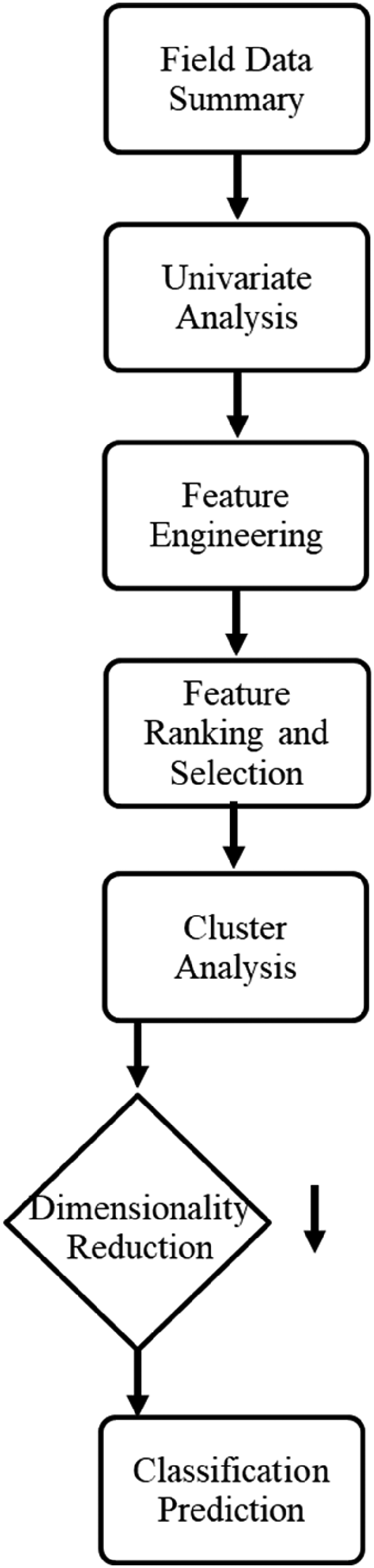
Proposed workflow for data-driven determination and classification of production profile types in unconventional reservoirs.

Our data-driven determination of production profile type steps consists of the following steps:

Field data summary—Perform a structured overview that includes geological and reservoir engineering settings to understand the scope and completeness of the dataset.

Univariate analysis—Assess the distributions, ranges, and potential outliers of both predictor features and response features.

Feature engineering—Apply normalization to completion design features to improve their information content.

Feature ranking and selection—Rank input features based on their relevance to the response feature and redundancy with other predictor features and select a reduced set of features to enhance model performance and interpretability.

Cluster analysis—Apply clustering techniques to group similar observations and reveal inherent structures in the dataset.

Dimensionality reduction—Use the MDS method to reduce feature dimensionality while preserving important variance and structures.

Classification prediction—Train classification models using selected features and reduced dimensions, evaluate their performance, and apply partial dependence plot (PDP) sensitivity analysis.

Field data summary systematically reviews the dataset in the context of geological and reservoir engineering characteristics to ensure spatial and temporal coverage is sufficient and representative for analysis. Next, univariate analysis is conducted to explore statistical distributions, validate feature ranges, and detect potential outliers in both predictor and response features. Feature engineering includes the application of normalization techniques—particularly to completion design features—to enhance model interpretability and ensure comparability across wells with varying scales and operational parameters.

Feature ranking methods evaluate the relevance of each predictor feature with respect to the response feature or its redundancy with other predictor features. Feature ranking and selection are applied to identify the most informative subset of predictor features to maximize model accuracy and model interpretability. A wide array of metrics is applied for feature ranking and selection, including correlation analysis, including Spearman's rank correlation coefficient, partial correlation coefficient, and canonical correlation coefficient, VIF to quantify multicollinearity, MRMR with mutual information to balance predictive relevance and redundancy under nonlinear dependencies, RFE, and model-based feature importance derived from ensemble learning models. Each metric provides unique information about feature relevance and redundancy, the nature of the relationships, and the impacts of outliers, confounding features and nonlinearity. Features consistently ranked as highly relevant across multiple metrics are retained, while features exhibiting strong redundancy are removed.

Clustering is an inferential and unsupervised ML method without response feature labels to automate the segmentation of the data into groups, known as clusters and specified by unique integer indices. Mixing distinct populations during model training often reduces predictive accuracy; thus, these cluster labels are used as inputs for production type classification models. We apply the K-means clustering algorithm, which minimizes dissimilarity within clusters. The number of clusters, K, is a hyperparameter that can be selected using expert knowledge or methods such as the elbow or silhouette method. Specifically, the elbow method is used to examine the marginal reduction in within-cluster sum of squares with increasing K, the Calinski–Harabasz index is employed to quantify the ratio of between-cluster to within-cluster variance, with larger values indicating more compact and better-separated clusters. Candidate values of K are further screened to ensure geological and production interpretability. Based on these criteria, the selected value of K represents a balance between statistical compactness and physically meaningful segmentation of production behavior.

MDS provides an effective approach to reduce the dimensionality of high-dimensional and complex datasets by transforming the original high-dimensional predictor feature space into a lower-dimensional space, typically two or three dimensions. The motivation for applying MDS is to establish a more interpretable and intuitive representation of relationships between wells, capturing the essential structure inherent in their pairwise dissimilarities. Specifically, MDS takes the matrix of pairwise dissimilarities among wells by preserving pairwise dissimilarities in the reduced space. Specifically, MDS takes a dissimilarity matrix based on predictor features and performs a nonlinear projection to minimize the difference between original and projected distances. This allows for both global and local structures to be retained, supporting a more meaningful interpretation of well relationships. Unlike linear methods such as PCA, MDS can accurately represent nonlinear relationships, making it particularly suitable for datasets with complex nonlinearity patterns. This improved representation enhances subsequent analyses and downstream tasks, such as clustering or classification, by facilitating easier visualization and interpretation of patterns, outliers, and intrinsic groupings within the data.

Random forest is an ensemble tree-based method that constructs multiple decision trees to improve predictive accuracy and it is employed for classification prediction tasks. To interpret and visualize the behavior of these classifiers, a PDP is utilized. PDP illustrates the average predicted response of the classifiers as a function of individual predictor features. This reveals how sensitive predictions are to specific features and clarifies their contribution to model outcomes.

Our proposed workflow integrates statistical exploration, feature selection, clustering, and dimensionality reduction to enable interpretable classification and pattern recognition in complex datasets. By systematically progressing from data summarization to model-driven analysis, the methodology ensures that key feature relationships and structural patterns are captured and leveraged in final predictive tasks. The following section presents the results of applying this workflow, demonstrating its effectiveness through classification case studies and providing insight into its performance and interpretability.

Results

This section presents the results of ML inference and the prediction of production profile types.

Dataset description

The dataset includes 189 wells in the Permian Basin, including 178 horizontal wells, 9 vertical wells, and 2 directional wells, shown in Figure 2. These wells span eight distinct geological formations, with notable concentrations in Wolfcamp_B (89 wells), Wolfcamp_A (60 wells), and Wolfcamp_C (39 wells). In Figure 3, approximately 60% of the wells were completed before May 13, 2016, while the remaining 40% represent more recent completions. Notably, wells completed after May 13, 2016, generally exhibit higher cumulative oil production in their first year.

Figure 2.

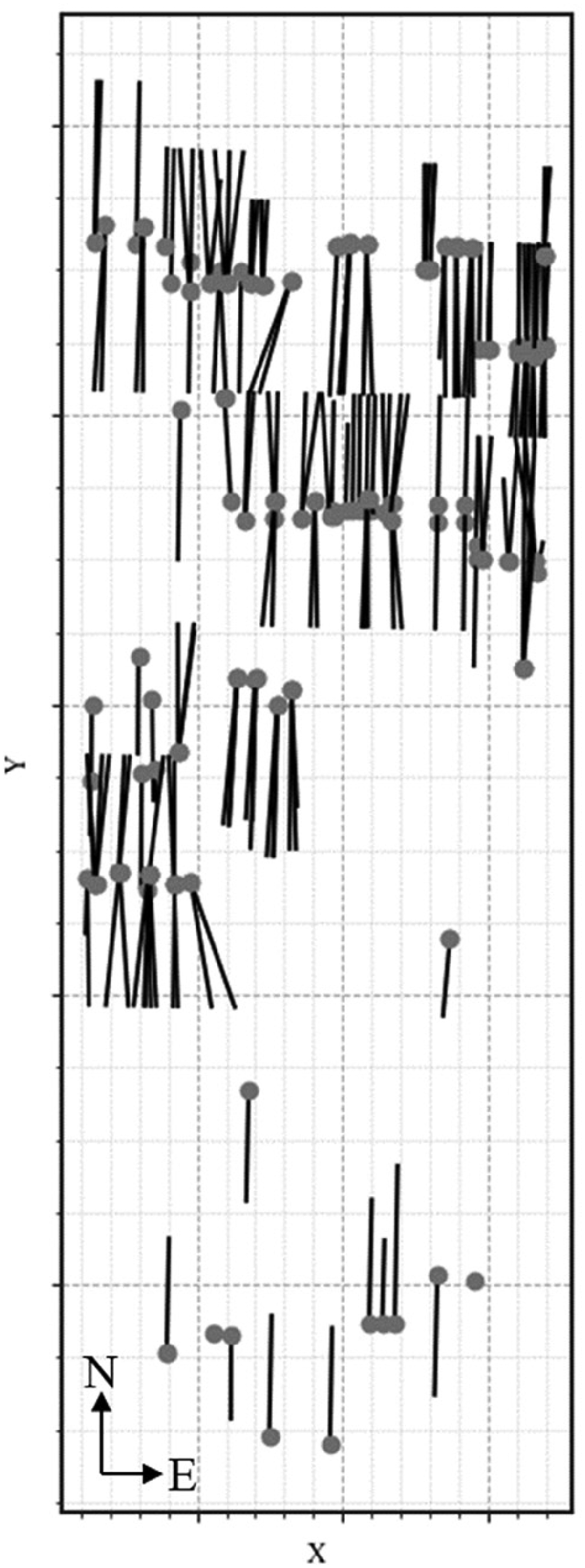
Location map of the 189 wells in the Permian Basin, including horizontal, vertical, and directional wells. Note. Axes units are omitted to support data anonymization.

Figure 3.

Distribution of 2-year cumulative oil production by well completion date.

Feature normalization and univariate analysis

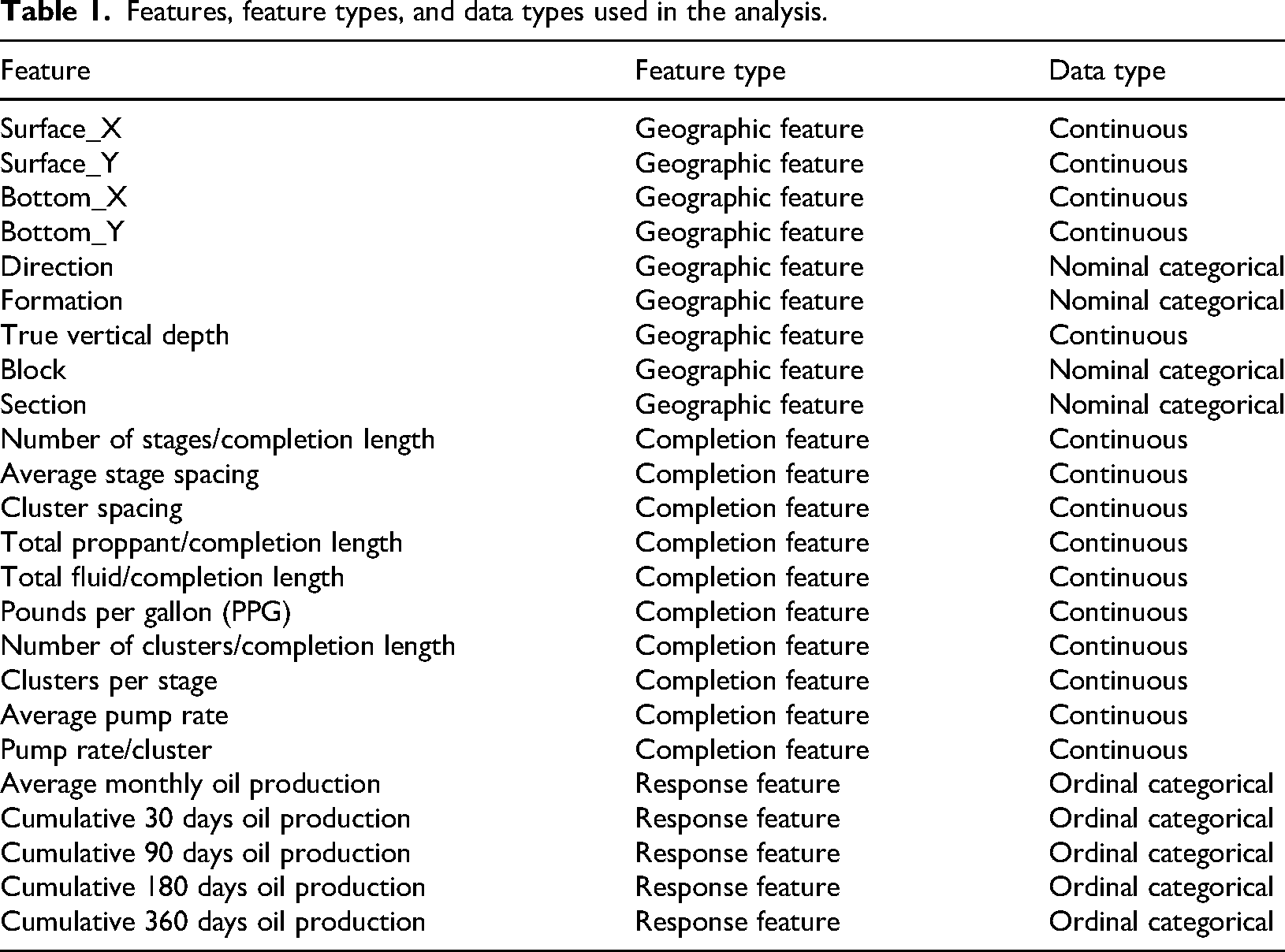
In Table 1, the “Feature” column lists all predictor and response features used in this analysis. Number of stages, total proppant, total fluid, and number of clusters are normalized by completion length to emphasize completion intensity metrics rather than absolute treatment volumes and measure depth, completion length, proppant per linear foot, and fluid per linear foot are removed from predictor features which are redundant with the remaining features. Correspondingly, the features are grouped into three types: geographic features, completion features, and response features. Direction, formation, block, and section information are represented as nominal categorical labels, and all other features are continuous and ordinal categorical features.

Table 1.

Features, feature types, and data types used in the analysis.

Feature	Feature type	Data type
Surface_X	Geographic feature	Continuous
Surface_Y	Geographic feature	Continuous
Bottom_X	Geographic feature	Continuous
Bottom_Y	Geographic feature	Continuous
Direction	Geographic feature	Nominal categorical
Formation	Geographic feature	Nominal categorical
True vertical depth	Geographic feature	Continuous
Block	Geographic feature	Nominal categorical
Section	Geographic feature	Nominal categorical
Number of stages/completion length	Completion feature	Continuous
Average stage spacing	Completion feature	Continuous
Cluster spacing	Completion feature	Continuous
Total proppant/completion length	Completion feature	Continuous
Total fluid/completion length	Completion feature	Continuous
Pounds per gallon (PPG)	Completion feature	Continuous
Number of clusters/completion length	Completion feature	Continuous
Clusters per stage	Completion feature	Continuous
Average pump rate	Completion feature	Continuous
Pump rate/cluster	Completion feature	Continuous
Average monthly oil production	Response feature	Ordinal categorical
Cumulative 30 days oil production	Response feature	Ordinal categorical
Cumulative 90 days oil production	Response feature	Ordinal categorical
Cumulative 180 days oil production	Response feature	Ordinal categorical
Cumulative 360 days oil production	Response feature	Ordinal categorical

The average monthly oil production is summarized using probability density function and cumulative distribution function plots in Figure 4. This univariate analysis on the well scale shows that more than 80% wells have cumulative 2-year oil production of less than 150,000 BBL.

Figure 4.

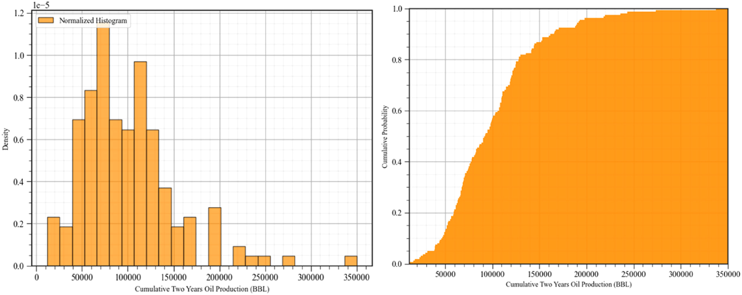
Probability density function (left) and cumulative distribution function (right) of cumulative 2-year oil production.

Feature ranking and selection

First, we apply canonical correlation analysis to select the response feature between oil production and gas production. Through computing canonical correlations, oil production (with a value of 0.9120) emerges as a better response feature than gas production (with a value of 0.7107). In order to select the optimal response features among different oil production features, we perform a correlation analysis (Figure 5). Considering the improved mapping to value and likely smoother behavior, we analyze cumulative oil production instead of average monthly oil production. One predictor feature, the normalized number of clusters, is used to evaluate how rank and partial correlations change with different response features. As the number of days for cumulative oil production increases, both rank and partial correlations increase as well. Cumulative oil production over 2 years shows the highest rank and partial correlations, and is therefore used as the response feature in the proposed workflow.

Figure 5.

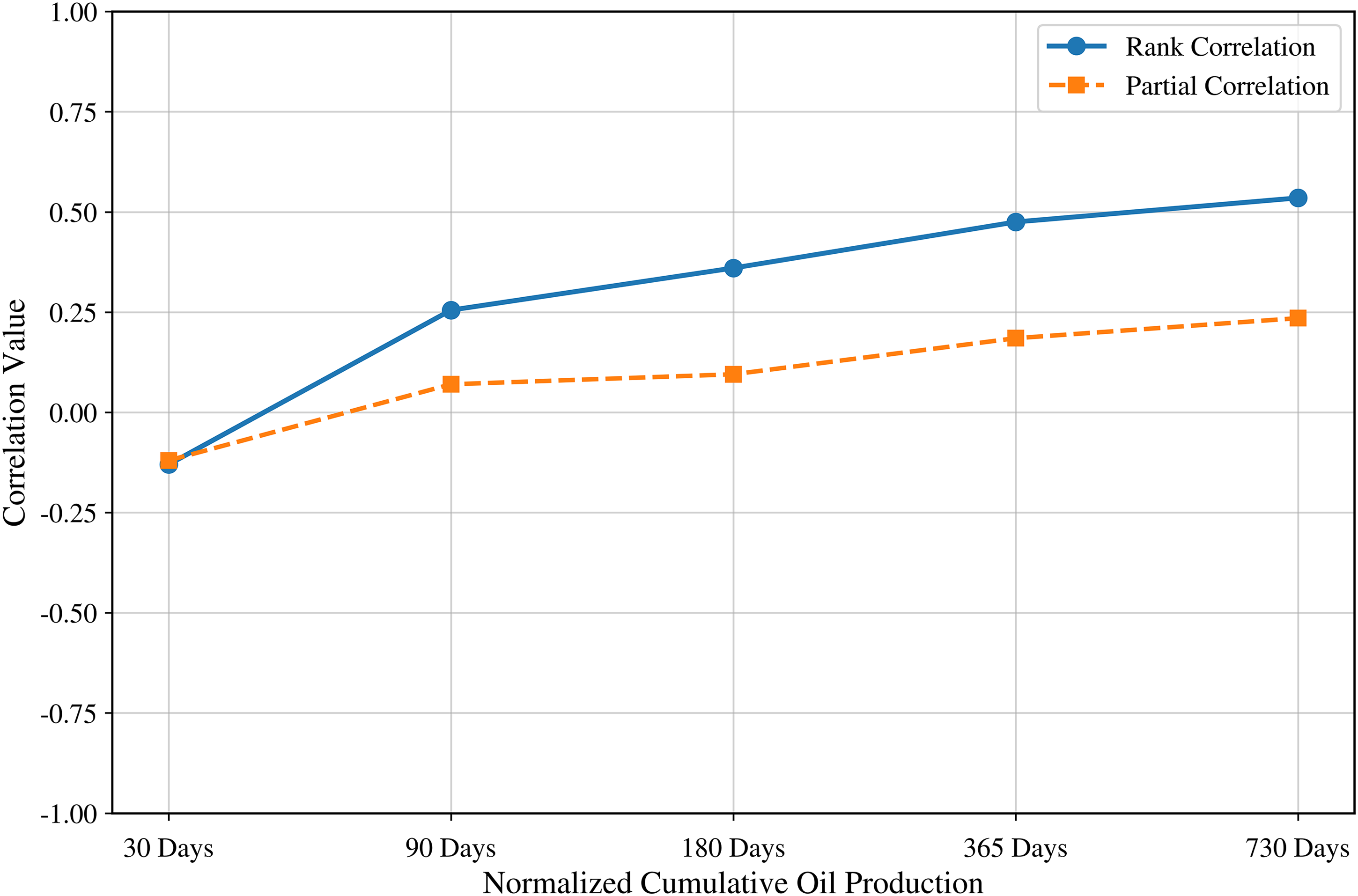
Correlation results between the normalized number of clusters and various response features.

Multivariate analysis, including the pairwise Spearman rank correlation coefficient and partial correlation coefficient, is applied to evaluate the strength of the relationship between the predictor features and the response feature (Figure 6). The advantage of pairwise Spearman rank correlation is its robustness to outliers in the dataset because it relies on the ranks of the data rather than their raw values, unlike covariance, which is sensitive to extreme values and assumes linear relationships between features. Normalized number of stages, number of clusters, total proppant, total fluid, and clusters per stage show high positive rank correlations with the response feature, the cumulative 2-year oil production. In contrast, average stage spacing, cluster spacing, and pump rate/cluster show strong negative correlations with cumulative 2-year oil production. The right plot in Figure 6 shows the partial correlation coefficients between predictor features and the response feature. These correlations are generally lower because the partial correlation removes the effects of all remaining predictor features. This allows for the evaluation of the direct association between each predictor and the response feature, excluding confounding effects from others. Among the predictor features, average pump rate, cluster spacing, normalized number of stages, number of clusters, total proppant, total fluid, and clusters per stage show relatively higher correlations compared to others.

Figure 6.

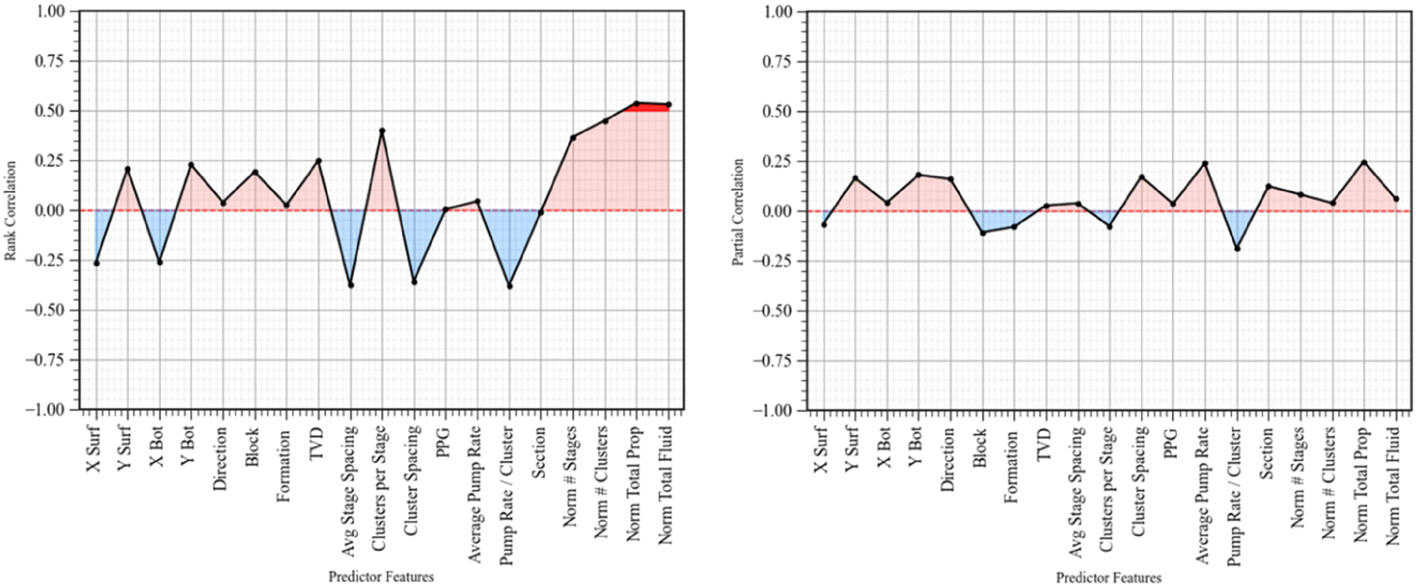
Pairwise Spearman rank correlation coefficients (left) and partial correlation coefficients (right) between predictor features and cumulative 2-year oil production.

Because we have 19 predictor features, feature selection is essential to mitigate the curse of high dimensionality, which can degrade model performance by increasing model variance due to the inclusion of redundant features, overfitting risk due to data noise matched with increased model complexity (Figure 7). Feature ranking and selection are based on the integration of three methods, which are the MRMR objective function, partial correlation coefficient, and VIF. MRMR calculates the average mutual information between the subset of predictor features and the response feature, minus the average mutual information among the predictor features. Typically, a higher MRMR value indicates more informative features that should be selected. As discussed previously, we also consider predictor features with high partial correlations. VIF measures the linear multicollinearity between a predictor feature and all other predictor features, so a high VIF represents high feature redundancy, indicating a lower feature rank. Based on these criteria, normalized total proppant, normalized total fluid, normalized number of clusters, pump rate per cluster, cluster spacing, clusters per stage, and average stage spacing are identified as important features.

Figure 7.

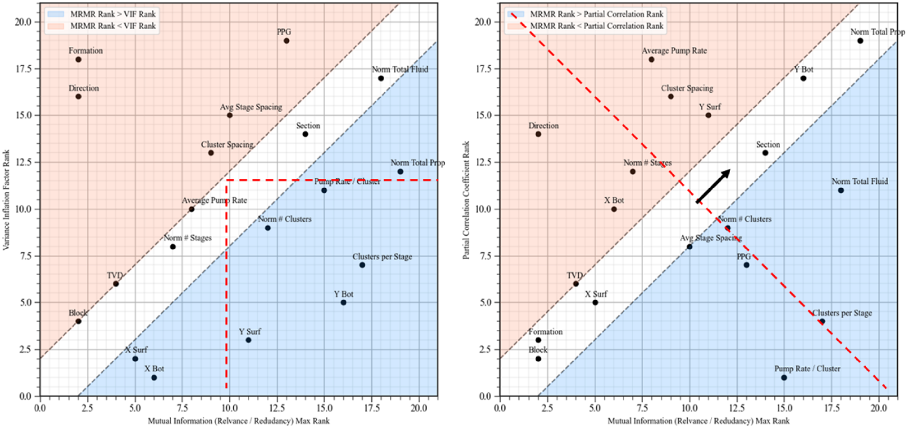
Variance inflation factor versus mutual information (relevance/redundancy) max ranking (left) and partial correlation versus mutual information (relevance/redundancy) max ranking (right). The shaded red area indicates cases where the MRMR rank is lower than the corresponding VIF and partial correlation rank, while the shaded blue area represents cases where the MRMR rank is higher than the VIF and partial correlation rank. MRMR: maximum relevance–minimum redundancy; VIF: variance inflation factor.

Besides using the plot above to compare feature ranking information between two feature ranking methods, Figure 8 further illustrates the difference between MRMR rank, VIF rank, and partial correlation rank. In the left plot, the completion features such as normalized total proppant, normalized number of clusters, cluster spacing, and pump rate per cluster show a positive difference between MRMR rank and VIF rank, indicating that inclusion of relevance along with nonlinear structures improves their ranks, In the right plot, the y-axis represents the difference between MRMR rank and partial correlation rank, and positive values indicate that integration of nonlinear structures increases the rank. Importantly, we also refer to Figure 6, as features with both low MRMR and low partial correlation ranks may result in a near-zero difference—potentially masking their limited usefulness. This highlights the need to interpret Figure 8 in conjunction with earlier correlation analysis (Figure 6) and redundancy metrics (Figure 7) for a more complete assessment of feature importance.

Figure 8.

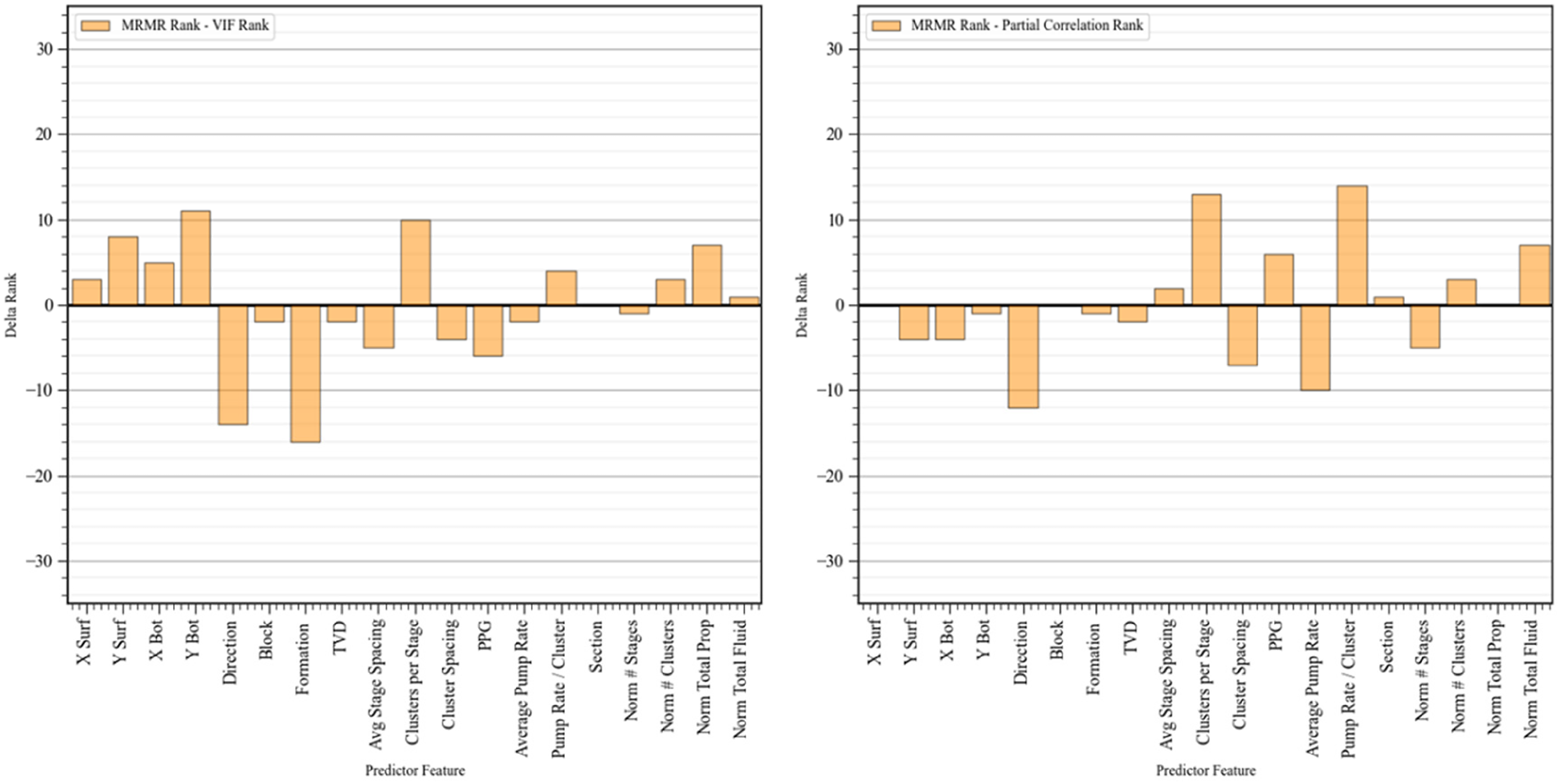
Difference between MRMR ranking and VIF ranking (left), and between MRMR ranking and partial correlation ranking (right). MRMR: maximum relevance–minimum redundancy; VIF: variance inflation factor.

We also investigate the impact of normalization on four predictor features and the response feature. As a result, the MRMR metrics of all predictor features drop after normalization. Figure 9 reveals that the relevance between predictor features and the response feature decreases, and the redundancy between predictor features increases because of normalization by completion length. We also note that MRMR metrics and rank correlations for the number of stages, the number of clusters, total proppant, and total fluid decline significantly because these four predictor features are normalized by completion length, which weakens their relationships with the response feature.

Figure 9.

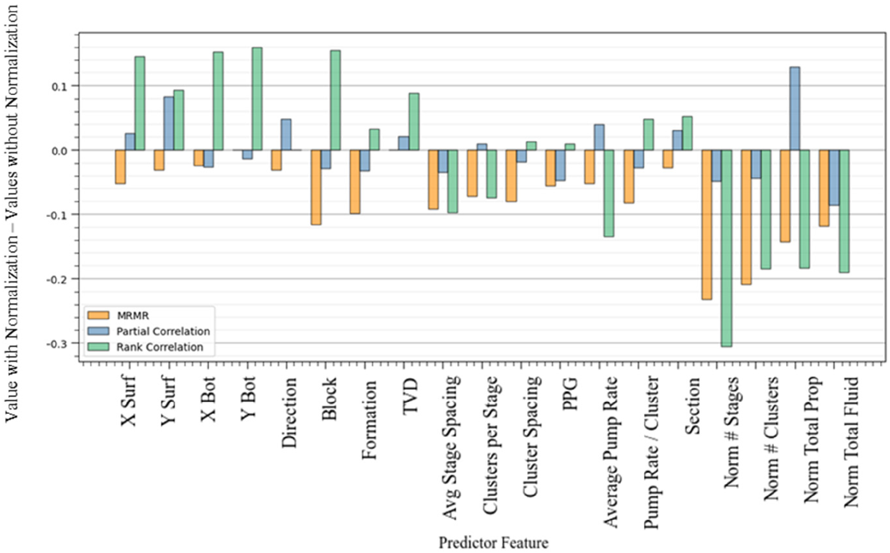
Effect of normalization on the relevance and redundancy of predictor features.

RFE method works by recursively removing the weakest feature and recalculating the feature ranks with the remaining features, and repeating the process until only one feature remains. Features eliminated later in the process are considered more important, and ranks are assigned in the reverse order of elimination. For instance, the first feature eliminated receives the lowest rank, while the last feature remaining receives the highest rank. The benefit of RFE is that it does not discard features solely based on redundancy if they also exhibit high relevance. This behavior is visualized in a novel RFE plot that shows the MRMR metric over the elimination step. For example, Figure 10 illustrates noticeable increases in the MRMR score for normalized proppant as other redundant features are eliminated.

Figure 10.

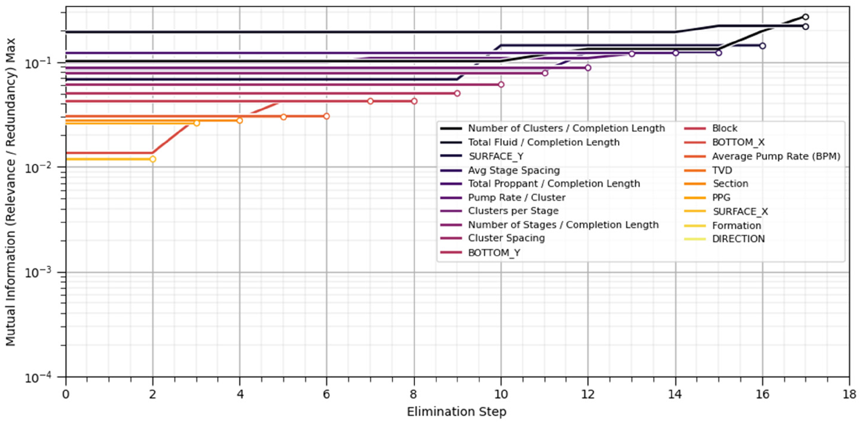
MRMR metric plotted across RFE steps using a one-factor-at-a-time (OFAT) approach. MRMR: maximum relevance–minimum redundancy; RFE: recursive feature elimination.

A model-based random forest method is also applied to rank the features with feature importance scores calculated based on each feature's contribution to reducing the prediction loss function. Since model-based feature ranking depends on the quality of the predictive model, it is important to visualize the model's performance on testing data, as shown in the comparison plot between actual and predicted values (left panel of Figure 11). Given the acceptable prediction performance, the model-based ranking is considered (right panel of Figure 11), identifying the top predictor features as normalized total proppant, total fluid, number of clusters, cluster spacing, pump rate per cluster, and clusters per stage. Based on the combined results of all prior feature ranking and selection methods, we identify six important predictor features for use in the remainder of our proposed workflow, which are normalized total proppant, normalized number of clusters, pump rate per cluster, pounds per gallon (PPG), cluster spacing, and average stage spacing. These features are carried forward into subsequent steps, including cluster analysis, dimensionality reduction, and the case study.

Figure 11.

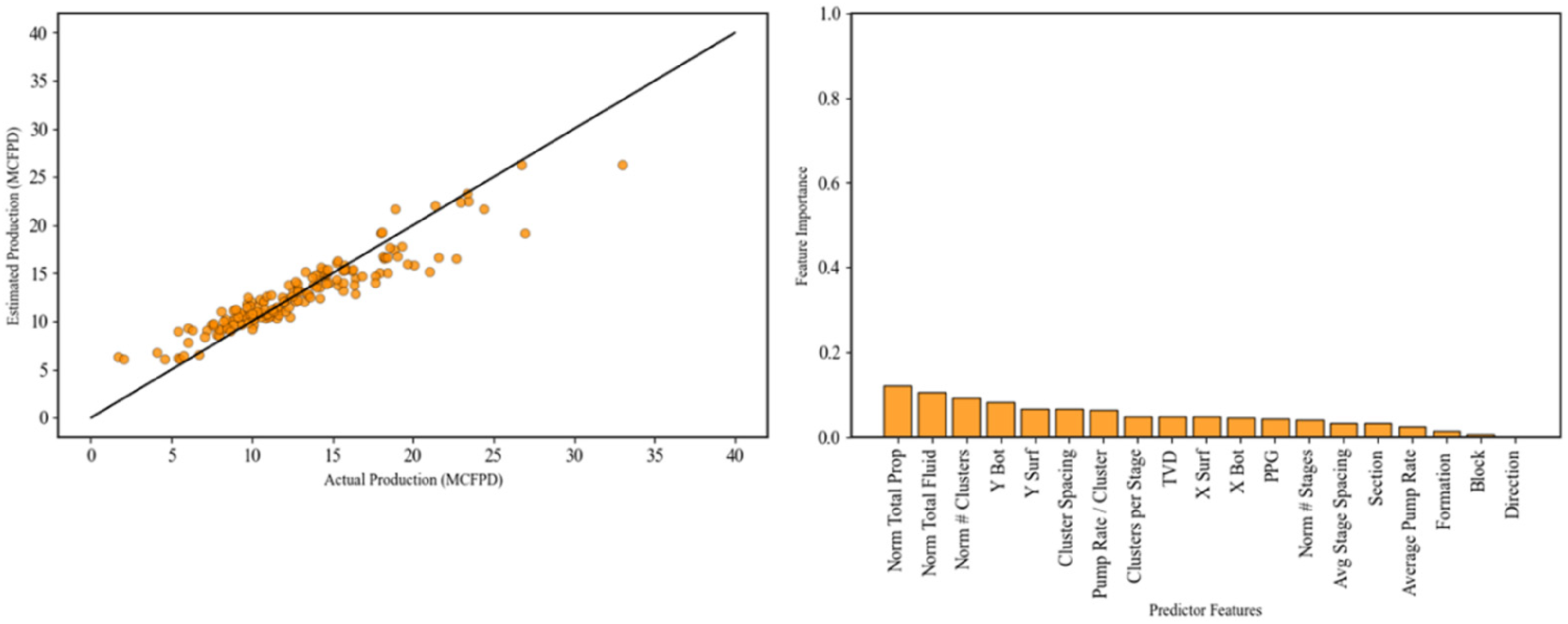
Actual versus predicted values from the random forest model (left), and feature importance scores for predictor features based on model performance (right).

Cluster analysis

Clustering is an inferential ML method for automatic segmentation of distinct populations. It is often applied prior to predictive modeling, allowing population-specific models to be developed, each with improved accuracy. The K-means clustering algorithm is used as the primary unsupervised learning method for this task. It assigns group labels to unlabeled data by minimizing dissimilarity within clusters. In our analysis, K-means divides the dataset into two clusters (Figure 12). Cluster 1, shown in purple, contains data points with relatively higher values of normalized total proppant and number of clusters, while cluster 2, shown in yellow, contains data with relatively lower values of these features. To determine the optimal number of clusters (the K hyperparameter), we apply the elbow method, which identifies the inflection point on the inertia versus number of clusters plot (middle panel of Figure 12). The inertia curve shows a pronounced decrease between K = 1 and K = 2. The Calinski–Harabasz index attains its highest value at K = 2 among cluster counts (K < 10) (right panel of Figure 12). Values of K larger than 10 lead to oversegmentation into subgroups with limited operational relevance and reduced interpretability. Additionally, our focus is on obtaining a parsimonious and interpretable partition in unconventional reservoir development. The two-cluster solution captures the major separation structure in the data while avoiding oversegmentation of what are effectively two dominant behavioral groups. We therefore selected K = 2 as the optimal number of clusters.

Figure 12.

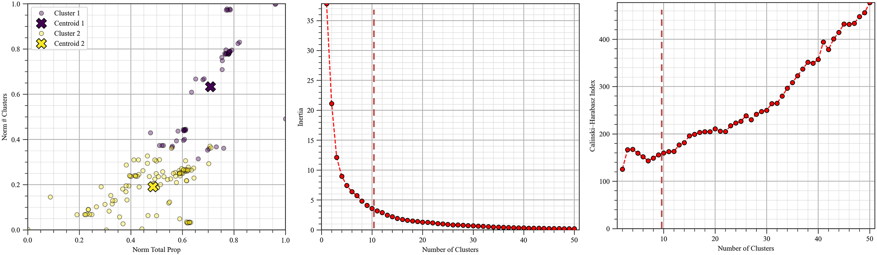
K-Means clustering results: two-cluster grouping based on six predictor features (left), and inertia (middle) and Calinski–Harabasz index versus number of clusters used to determine the optimal K value (right).

To evaluate the physical interpretability of the K-means clustering results, we examine how completion feature attributes differ between the two identified clusters. Figure 13 compares the number of clusters per completion length and cluster spacing for each K-means cluster. Wells assigned to cluster 1 exhibit higher mean cluster density and tighter cluster spacing, and cluster 2 is characterized by lower cluster density and wider cluster spacing. The clear separation in these physically meaningful completion features demonstrates that the unsupervised K-means clustering is not arbitrary, but instead captures operationally interpretable differences in completion features that are expected to influence production performance.

Figure 13.

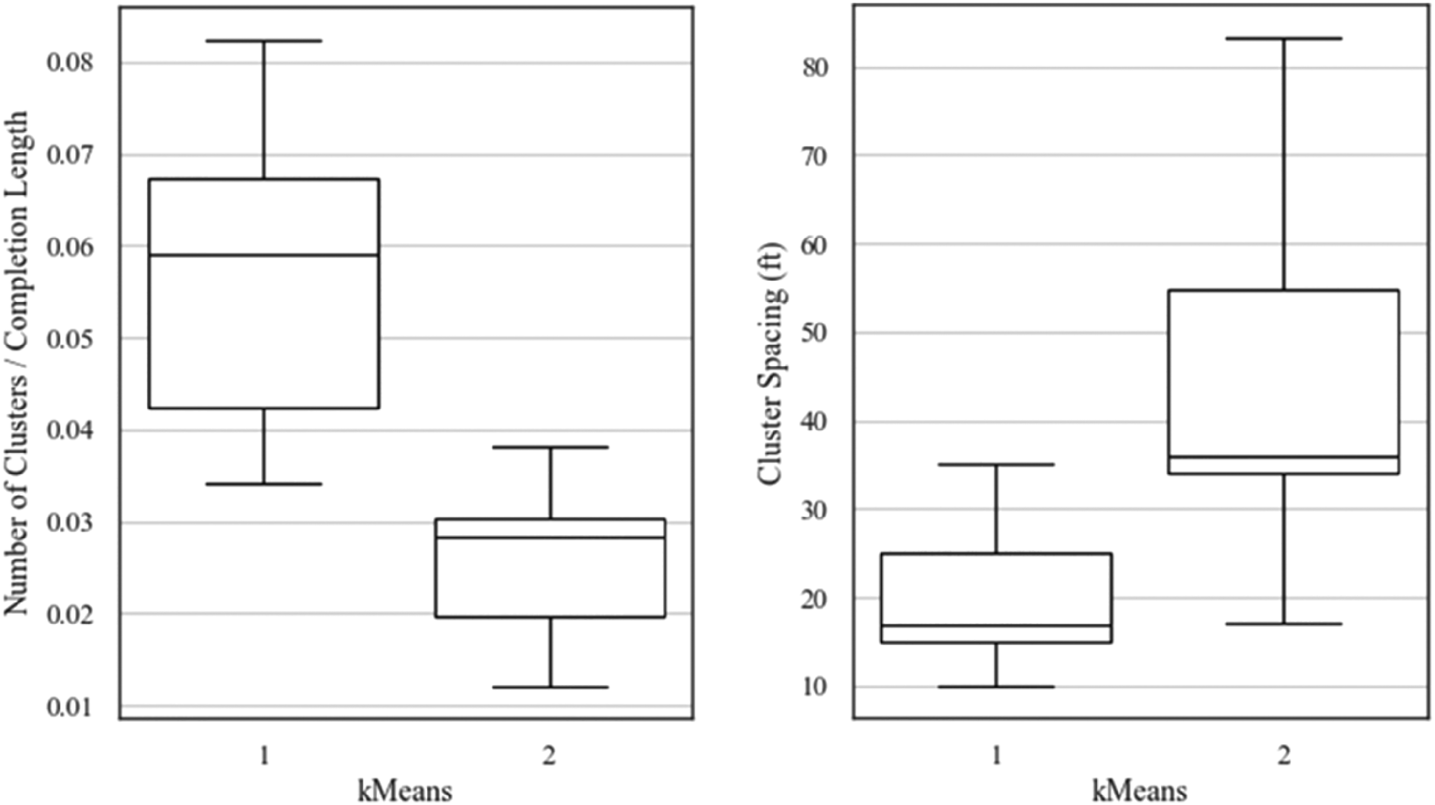
The box plots of the number of clusters per completion length (left) and cluster spacing (right) by K-means cluster.

As previously mentioned, K-means clustering is an unsupervised ML method, which means the response feature is not used during the clustering process. After obtaining the two cluster groups in Figure 12, we analyze how the normalized oil production histories of wells differ across these clusters. To do this, we calculate the conditional expectation and percentiles of production over time by cluster group, demonstrating a clear separation between clusters 1 and 2, allowing us to assign wells in cluster 1 with the type of “high production” and those in cluster 2 with the type of “low production” (Figure 14). Due to the variation in production periods across wells, we truncate the x-axis to a maximum production duration of 63 months. This prevents data loss and eliminates the need for missing value imputation, thereby reducing potential bias in the analysis.

Figure 14.

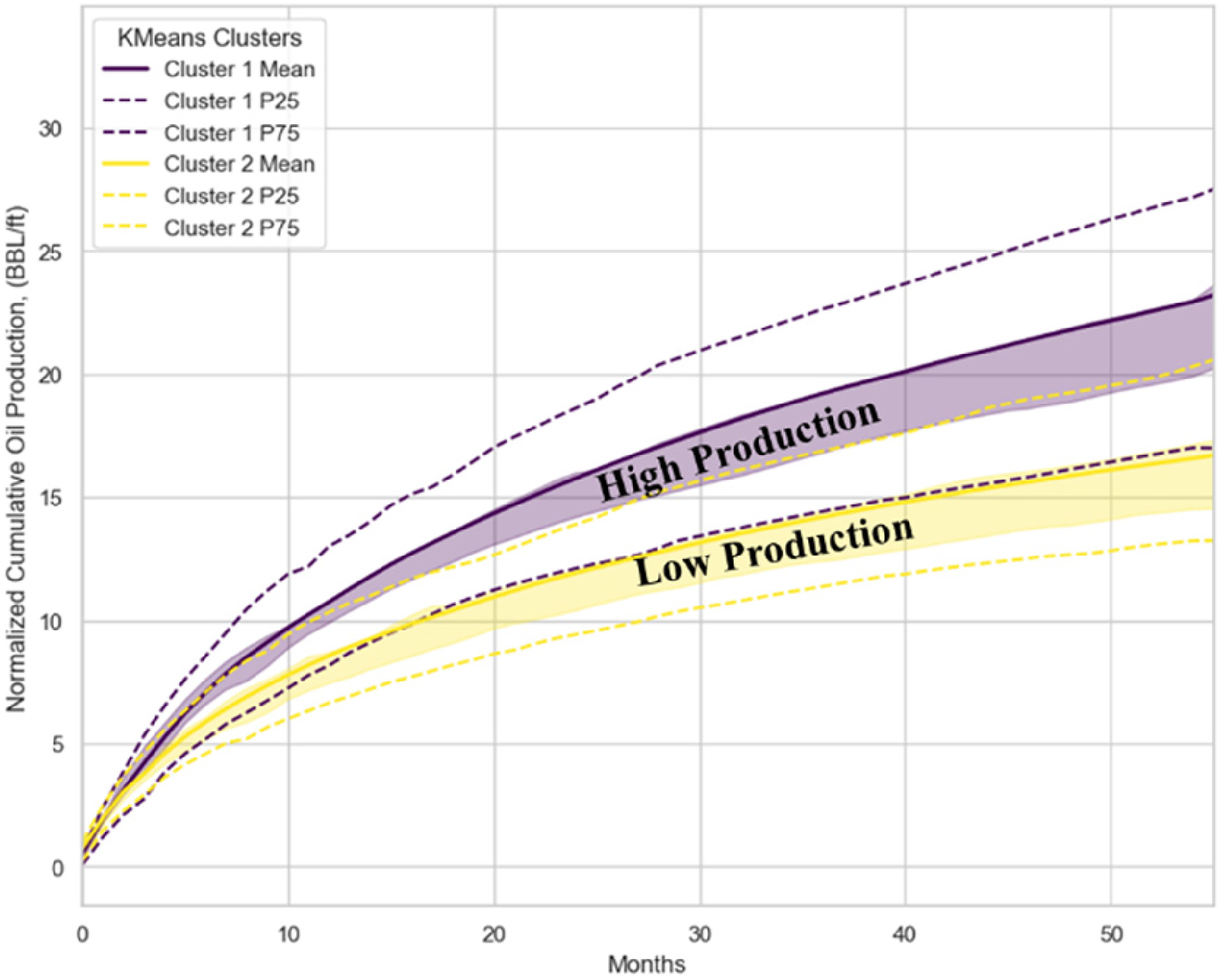
Normalized oil production history for the two K-means clusters. The shaded area represents the P40–P60 range of wells within each cluster, while dashed lines indicate the P25 and P75 percentiles.

Dimensionality reduction-multidimensional scaling (MDS)

Previously, we performed feature ranking and selection to reduce the number of predictor features from 19 to 6. However, it is still difficult to visualize the relationships within our datasets with more than two or three features. MDS addresses this issue by operating on a distance or dissimilarity matrix, projecting high-dimensional data into a two-dimensional feature space. A key advantage of MDS is that it does not require the actual feature values—only the pairwise dissimilarities between the samples. As shown in Figure 15, the MDS projection of wells, labeled by K-means cluster assignment, demonstrates clear separation between the two clusters, confirming the structure revealed through clustering.

Figure 15.

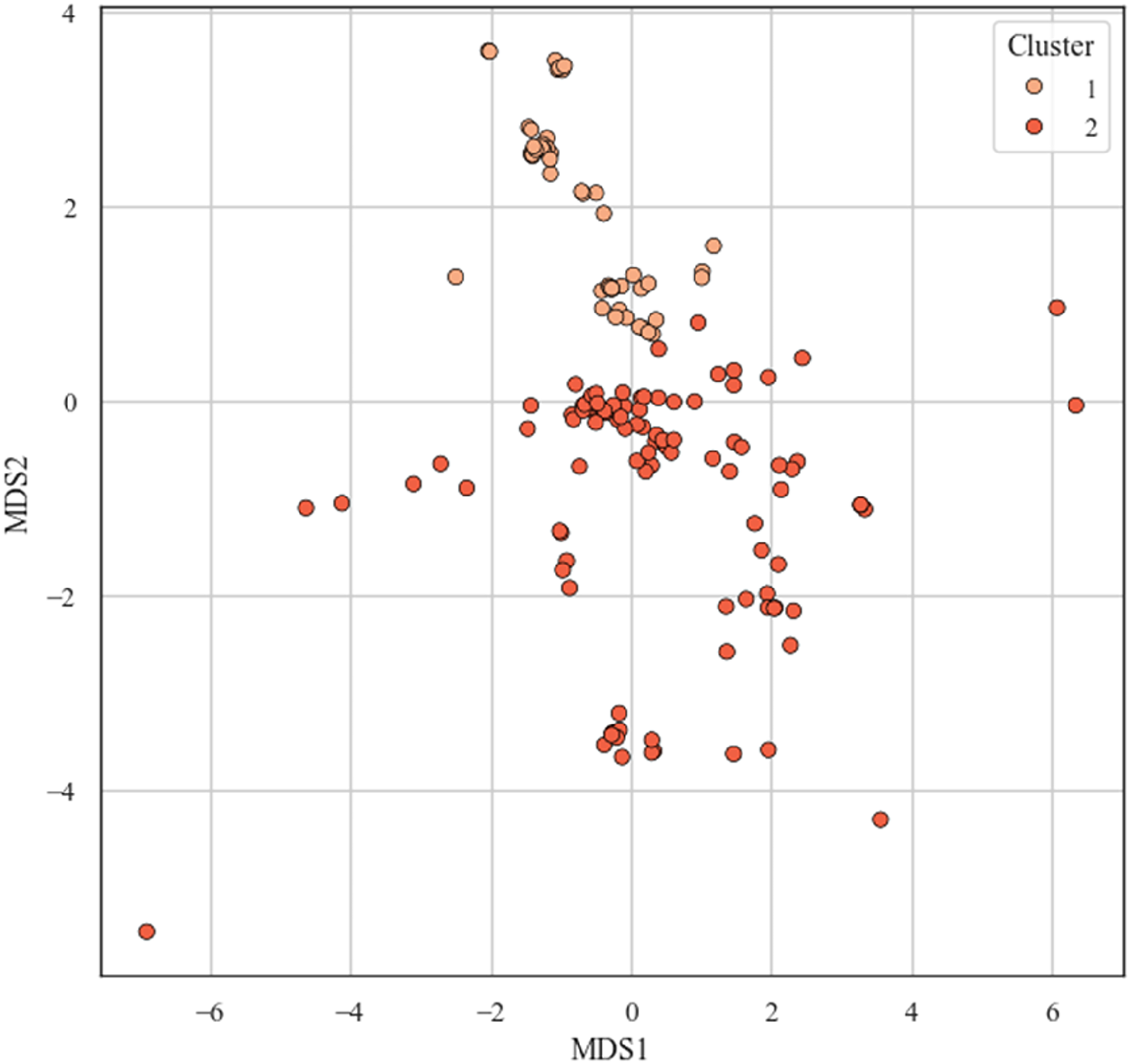
Visualization of wells in two-dimensional space using MDS based on the six selected predictor features. MDS: multidimensional scaling.

To evaluate the performance of MDS, we cross-plot the pairwise distance between the original high-dimensional space and the projected two-dimensional space (Figure 16). Most points lie close to the 45-degree line, indicating that pairwise dissimilarities are well preserved in the MDS projection.

Figure 16.

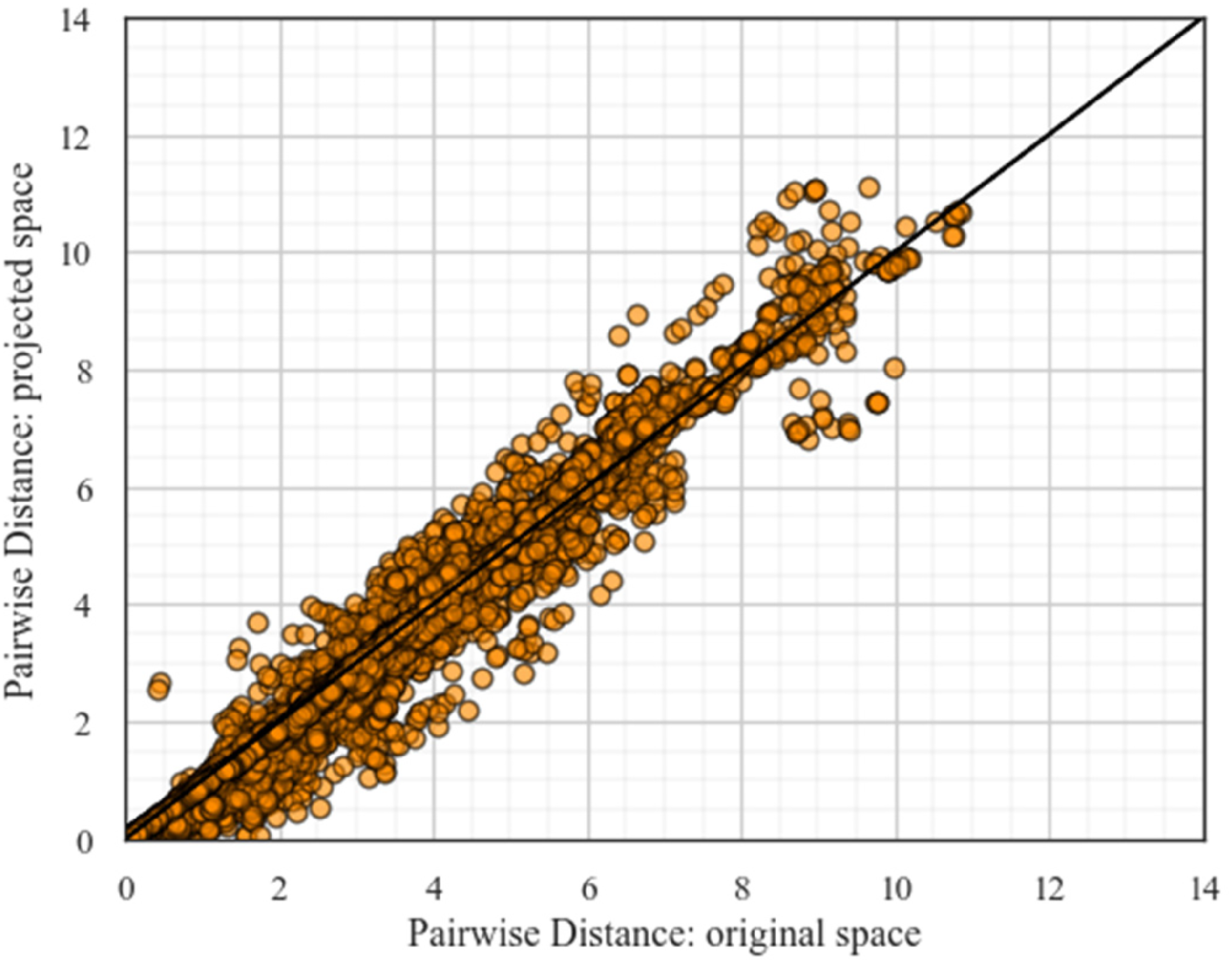
Evaluation of MDS performance by comparing pairwise distances in the original high-dimensional space and the projected two-dimensional space. MDS: multidimensional scaling.

Classification prediction and PDP sensitivity analysis

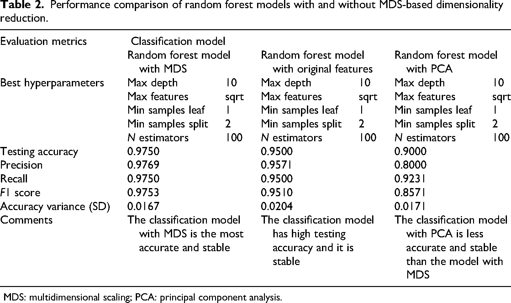
We apply the random forest tree-based classifier to build a prediction model for production curve type with low and high production using the low-dimensional MDS1 and MDS2 features. The dataset is split into 75% training and 25% testing subsets and the distribution of wells across formations remained consistent between splits to avoid the risk of spatial leakage. To check the impact of dimensionality reduction via MDS, we compare this model's performance to a tuned random forest model training on the original top-ranked six predictor features and a tuned random forest model with the linear dimensionality-reduction PCA. The first two principal components of PCA are used as inputs to the classifier to ensure a consistent comparison with the two-dimensional MDS embedding. In three cases, the random forest models are tuned to the same hyperparameters. However, the model trained with MDS-transformed features achieves the highest testing accuracy (0.9750) compared to the model trained with original features (0.9500) and the model with PCA (0.9000), resulting in a 50% reduction in the probability of misclassification compared to the model trained with original features (i.e. predicting a low-production well for a high-production well and vice versa from 5% to 2.5%) and a 75% reduction in the probability of misclassification compared to the model trained with PCA (i.e. predicting a low-production well for a high-production well and vice versa from 10% to 2.5%). Furthermore, the model using MDS exhibits the lowest accuracy variance, with a standard deviation of 0.0167, compared to 0.0204 for the model with original features and 0.0171 for the model with PCA. This suggests that the random forest model trained on MDS features is not only more accurate but also more stable (Table 2, Figure 17). To further assess the robustness of this improvement, stratified four-fold cross-validation is performed using identical train–test splits for both models. Across folds, the MDS-based model achieves a higher mean testing accuracy (0.9875) than the model with original features (0.9812) and the model with PCA (0.9688), with comparable variability (standard deviations of 0.0217, 0.0207, and 0.0410, respectively), confirming that the observed performance gain persists beyond a single train–test split.

Figure 17.

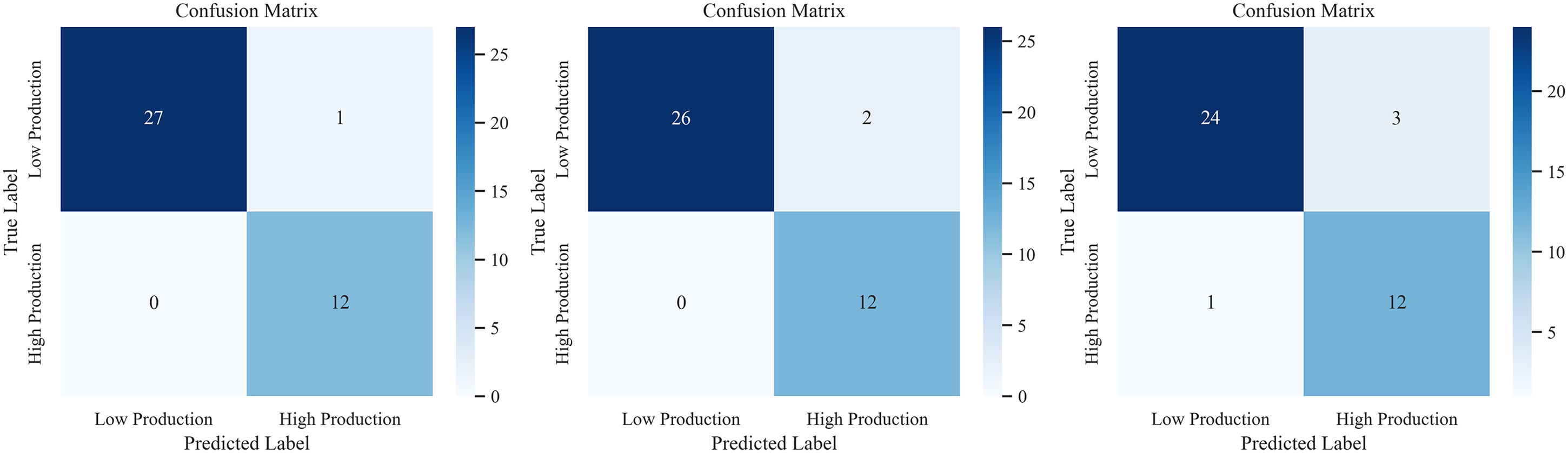
Confusion matrices for random forest models: with MDS-based features (left), with original features (middle) and with PCA-based features (right). MDS: multidimensional scaling; PCA: principal component analysis.

Table 2.

Performance comparison of random forest models with and without MDS-based dimensionality reduction.

Evaluation metrics	Classification model
	Random forest model with MDS		Random forest model with original features		Random forest model with PCA
Best hyperparameters	Max depth	10	Max depth	10	Max depth	10
	Max features	sqrt	Max features	sqrt	Max features	sqrt
	Min samples leaf	1	Min samples leaf	1	Min samples leaf	1
	Min samples split	2	Min samples split	2	Min samples split	2
	N estimators	100	N estimators	100	N estimators	100
Testing accuracy	0.9750		0.9500		0.9000
Precision	0.9769		0.9571		0.8000
Recall	0.9750		0.9500		0.9231
F1 score	0.9753		0.9510		0.8571
Accuracy variance (SD)	0.0167		0.0204		0.0171
Comments	The classification model with MDS is the most accurate and stable		The classification model has high testing accuracy and it is stable		The classification model with PCA is less accurate and stable than the model with MDS

MDS: multidimensional scaling; PCA: principal component analysis.

The improvement in random forest accuracy with MDS may be due to a reduction in multicollinearity between original predictor features that can help reduce model variance. Additionally, the MDS-based model results in faster computation and makes it easier to visualize the prediction space. However, it is important to note that MDS is designed to preserve pairwise distances in the feature space, not to maximize class separation. As a result, in some cases, MDS may compress or obscure class-discriminative information during projection, potentially affecting model interpretability or classification performance.

To support engineering decision-making with the model, further feature importance and sensitivity analyses are necessary. For this purpose, we use the random forest model trained on the original six predictor features, as the MDS-based model, while effective, lacks physical interpretability due to the abstract nature of its transformed features. As a first step, we compute the model's in-built feature importance scores (Figure 18). The results show that the normalized number of clusters, cluster spacing, pump rate per cluster, and normalized total proppant exhibit the highest importance, indicating their strong influence on production classification.

Figure 18.

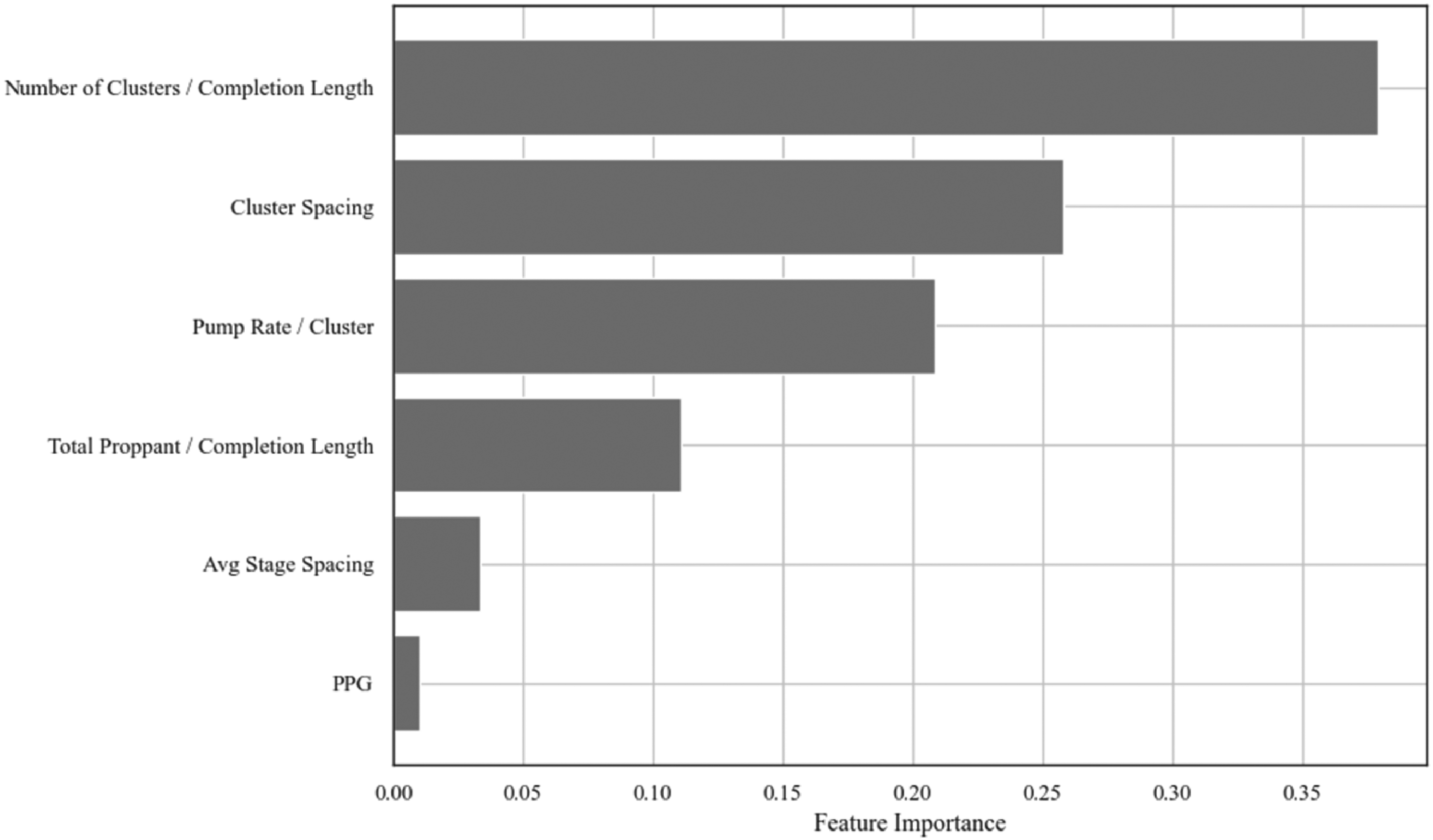
Feature importance scores from the random forest model using the original six predictor features.

PDP is a visualization technique used to understand the relationship between one or two features and the predictions of an ML model. It explains how the random forest classifier decides between low- and high-production curves, and represents an average effect over many hypothetical samples sharing only the same two selected features. All other confounding features are varied and averaged to remove their influence and then the expected model and contours are shown (Figure 19). We also calculate the offset distance from the original six dimensions to the two dimensions of each well. We note that when normalized total proppant increases above 2050, the normalized number of clusters increases above 0.038 and cluster spacing decreases below 35 ft, the oil production transitions from low to high production.

Figure 19.

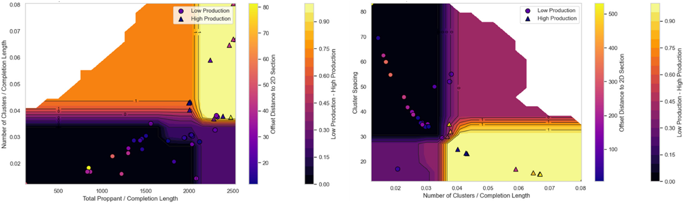
Partial dependence plot showing the relationship between two predictor features and oil production classification. A value of 0 indicates low production, and 1 indicates high production.

Additionally, we examine the relationship between a single predictor feature and oil production across all model predictions (Figure 20); for example, the impact of the change in the normalized number of clusters on the probability of a high-production response. This is also known as individual conditional expectation, which shows how samples’ predictions change as a single predictor feature varies, while holding other predictor features fixed. As a result, we identify a threshold for the normalized number of clusters around 0.038, and a threshold for cluster spacing around 35 ft.

Figure 20.

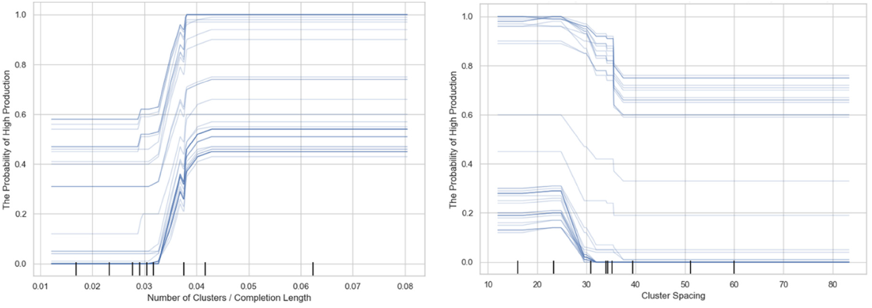
Probability of high production as a function of normalized number of clusters (left) and cluster spacing (right) across all testing wells.

With the trained prediction model, it is possible to select a single low-production well and then visualize the predictions across two predictor features to examine the decision boundary (i.e. how much change in the predictor features is required for the classification to switch from low to high production). This enables the selection of low-production samples of interest from the dataset to investigate potential changes in completion design that may improve well performance. For example, the well with index 14 is selected from the testing dataset, and we can directly observe how much each predictor feature—normalized number of clusters and normalized total proppant—would need to be increased to change the predicted classification to high production (Figure 21). In practice, such model-guided sensitivity visualization can support completion optimization and reservoir development planning by highlighting operational parameters (e.g. proppant loading, cluster density) that most influence production outcomes, and enables scenario-based “what-if” analysis, supporting development optimization, thereby guiding more cost-effective stimulation designs in future wells.

Figure 21.

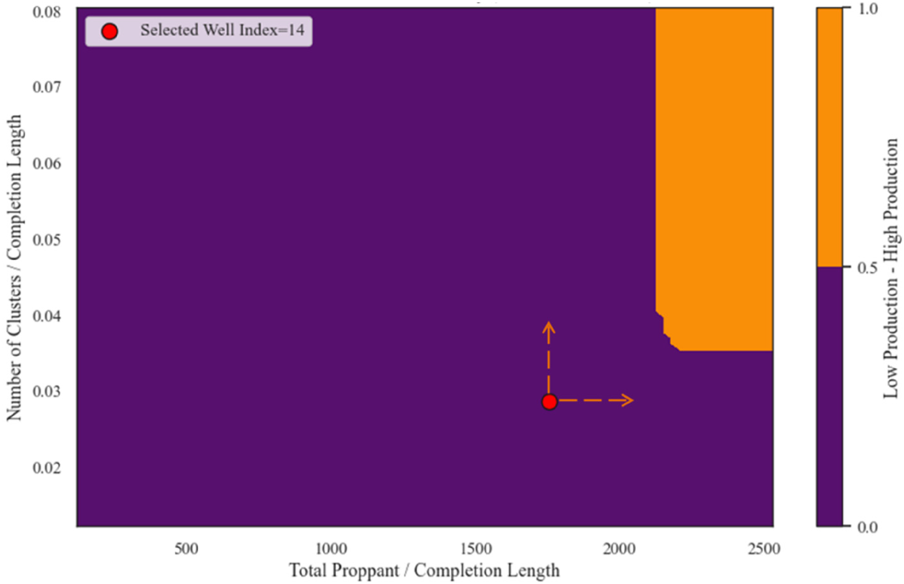
Random forest decision boundary for a single well, showing the required increases in normalized total proppant and normalized number of clusters to shift the classification from low production (purple) to high production (orange).

Conclusion

We propose a comprehensive ML workflow for unconventional reservoirs, enabling data-driven determination of production profile types through automatic clustering, group assignments, and then prediction of those group assignments. After applying multiple feature ranking and selection methods, including MRMR, VIF, partial correlation, RFE, and model-based methods, we select six predictor features, which are normalized total proppant, number of clusters, pump rate per cluster, PPG, cluster spacing, and average stage spacing. To reduce dimensionality and address feature redundancy, MDS is applied, projecting the selected predictor features into a two-dimensional space. MDS helps mitigate the curse of dimensionality and preserves pairwise distances between the samples. Cluster analysis on the MDS-reduced features identifies two distinct production types: low and high production. A classification model is then trained using these cluster-based labels. We observe that the use of MDS reduces multicollinearity among the original features and results in models that are equally or more accurate than those trained without MDS, while also achieving faster computation and lower running time. Among the features, normalized total proppant, normalized number of clusters, cluster spacing, and pump rate per cluster contribute most significantly to the random forest classifier. This supports engineering decision-making, which can be guided by insights from the PDPs using either two predictor features or one at a time, as well as the single-well decision boundary plot.

Our proposed workflow has practical applications for improved decision-making in the oil and gas industry. For example, it is possible to better identify the most important predictor features to focus data collection, develop optimum production profile groups to separate wells and prediction models with diagnostics to guide well site selection and completion design. However, several limitations should be acknowledged. First, the analysis is conducted on a moderate-sized dataset comprising 189 horizontal wells and 19 predictor features from the Permian Basin. More wells and features may further demonstrate the benefits of dimensionality reduction for the improvement of classification accuracy. Second, while MDS effectively reduces the dimensionality of correlated predictors, its transformed components are not directly interpretable in physical terms, limiting the ability to attribute specific engineering or geological mechanisms to each cluster boundary; therefore, in cases where principal components analysis is practical, it may be preferred for improved interpretability. Third, economic indicators and confidential production cost data are unavailable at this stage and are not incorporated into the current analysis. Inclusion of these variables can provide a more complete evaluation and decision-making of profitability and development optimization. Fourth, six predictor features used for clustering and classification are manually selected based on feature ranking and selection to retain the most informative and nonredundant features. While this selection reflects domain knowledge and statistical relevance, it is not unique, which can cause alternative combinations of predictor features derived from the same feature ranking and selection process. Nevertheless, the workflow remains applicable regardless of the specific predictors chosen, enabling adaptation to different datasets or operators’ preferences. Finally, a comprehensive uncertainty quantification and analysis of more geological data can be integrated.

Footnotes

Acknowledgment

The authors acknowledge University Lands management for their support and permission to publish this paper.

ORCID iDs

Dinghan Wang

Elnara Rustamzade

ORCID iD

Dinghan Wang

Funding

The authors disclosed receipt of the following financial support for the research, authorship, and/or publication of this article: The authors received financial funding from University Lands for this article.

Declaration of conflicting interests

The authors declared no potential conflicts of interest with respect to the research, authorship, and/or publication of this article.

Data availability statement

The data that support the findings of this study are not publicly available due to company confidentiality agreements.

References

Akmal

Pyrcz

(2025) New information theory measures for feature ranking for subsurface modeling (under review).

Alzahabi

Trindade

Kamel

(2023) Horizontal well completions using data analytics. Journal of Petroleum Science and Engineering 18: 101143.

Becht

McInnes

Healy

, et al. (2019) Dimensionality reduction for visualizing single-cell data using UMAP. Nature Biotechnology 37: 38–44.

Borg

Groenen

PJF

(2005) Modern Multidimensional Scaling: Theory and Applications. 2nd ed. New York: Springer.

Cheddad

(2023) Enhancing petrophysical studies with machine learning: A field case study on permeability prediction in heterogeneous reservoirs. arXiv, arXiv preprint arXiv:2305.07145. https://arxiv.org/abs/2305.07145 (accessed 10 May 2025).

Cheng

Cao

, et al. (2021) AI-based geo-engineering integration in unconventional oil and gas. Journal of King Saud University—Science 33: 6.

Huang

Wang

Rudin

, et al. (2022) Towards a comprehensive evaluation of dimension reduction methods for transcriptomic data visualization. Communications Biology 5: 719.

Hughes

(2013) Energy: A reality check on the shale revolution. Nature 494(7437): 307–308.

Hui-Mean

Chang

(2025) A survey: Potential dimensionality reduction methods. arXiv:2502.11036. 10.48550/arXiv.2502.11036.

10.

Jiang

Younis

(2015) A multimechanistic multicontinuum model for simulating shale gas reservoirs with complex fractured systems. Fuel 161: 882–897.

11.

Kruskal

Wish

(1978) Multidimensional Scaling. Beverly Hills: CA: Sage Publications.

12.

Liang

Zhao

(2019) A machine learning analysis based on big data for Eagle Ford Shale Formation. Presented at the SPE Annual Technical Conference and Exhibition, Calgary, Alberta, Canada, September 2019. SPE-196158-MS. https://doi.org/10.2118/196158-MS.

13.

Liu

Sun

Ngo

, et al. (2024) Machine learning-based completions sequencing for well performance optimization. arXiv, arXiv preprint arXiv:2402.15608. https://arxiv.org/abs/2402.15608 (accessed 10 May 2025).

14.

Mai-Cao

Truong-Khac

(2022) A comparative study on different machine learning algorithms for petroleum production forecasting. International Oil and Gas Research 1(1): 1–15.

15.

Merzoug

Chaparro

Burrough

, et al. (2025) A robust, model agnostic feature selection workflow for key performance drivers in unconventional reservoirs (under review).

16.

Pandian

(2025) Functional benefits of automating features using recursive feature elimination (RFE) and L1 medium. https://pandian-shanthababu.medium.com/functional-benefits-of-automating-features-using-recursive-feature-elimination-rfe-and-l1-941b0d1201d8 (accessed 10 May 2025).

17.

Pei

Xiong

(2022) Enhancing well performance and economic value via better well completion design—A Delaware Basin case study. SPE Journal 28(3): 934–949.

18.

Peng

Long

Ding

(2005) Feature selection based on mutual information: Criteria of max-dependency, max-relevance, and min-redundancy. IEEE Transactions on Pattern Analysis and Machine Intelligence 27(8): 1226–1238.

19.

Pyrcz

Deutsch

(2014) Geostatistical Reservoir Modeling. 2nd ed. New York: Oxford University Press.

20.

Silva

Ferreira

Avansi

, et al. (2023) Selection of a dimensionality reduction method: An application to deal with high-dimensional geostatistical realizations in oil reservoirs. SPE Reservoir Evaluation & Engineering 26(2): 392–410.

21.

Xiong

(2020) The effective cluster spacing plays a vital role in unconventional reservoir development—Permian Basin case studies. Presented at the SPE Hydraulic Fracturing Technology Conference and Exhibition, The Woodlands, Texas, USA, February 2020. SPE-199721-MS. https://doi.org/10.2118/199721-MS.

22.

Xiong

Liu

Feng

, et al. (2019) Optimizing fracturing design and well spacing with complex-fracture and reservoir simulations—A Permian Basin case study. Presented at the SPE Hydraulic Fracturing Technology Conference and Exhibition, The Woodlands, Texas, USA, February 2019. SPE-194367-MS. https://doi.org/10.2118/194367-MS.

23.

Xiong

Yoon

Jiang

(2021) A novel method to speedup calibrating horizontal well performance model with multi-stage fracturing treatments and its applications in Delaware Basin. Presented at the SPE Reservoir Simulation Conference, On-Demand, October 2021. SPE-203935-MS. https://doi.org/10.2118/203935-MS.

24.

Zhu

Forrest

Xiong

, et al. (2017) Cluster spacing and well spacing optimization using multi-well simulation for the Lower Spraberry Shale in Midland Basin. Presented at the SPE Liquids-Rich Basins Conference—North America, Midland, Texas, USA, September 2017. SPE-187485-MS. https://doi.org/10.2118/187485-MS.