Violations of Assumptions in School-Based Single-Case Data

Abstract

A wide variety of effect sizes (ESs) has been used in the single-case design literature. Several researchers have “stress tested” these ESs by subjecting them to various degrees of problem data (e.g., autocorrelation, slope), resulting in the conditions by which different ESs can be considered valid. However, on the back end, few researchers have considered how prevalent and severe these problems are in extant data and as a result, how concerned applied researchers should be. The current study extracted and aggregated indicators of violations of normality and independence across four domains of educational study. Significant violations were found in total and across fields, including low levels of autocorrelation and moderate levels of absolute trend. These violations affect the selection and interpretation of ESs at the individual study level and for meta-analysis. Implications and recommendations are discussed.

Keywords

effect sizes meta-analysis assumptions autocorrelation trend single subject

Recent legislation (e.g., Individuals With Disabilities Education Improvement Act, 2004; No Child Left Behind Act, 2002) as well as public and private entities (e.g., What Works Clearinghouse, The Wing Institute, Task Force on Evidence-Based Interventions in School Psychology) have prioritized the science of establishing evidence-based practice in education. As part of this dialogue, there has been renewed interest in developing the technology of effect sizes (ESs), significance testing, and research synthesis for single-case designs (SCDs; see reviews by Franklin, Allison, & Gorman, 1997; Levin, Ferron, & Kratochwill, 2012; Parker & Brossart, 2003; Parker, Vannest, & Davis, 2011; Shadish, Rindskopf, & Hedges, 2008). The purpose of such statistics is not to replace more venerable methods for determining outcomes with SCDs but to supplement them with a common language of effects.

There is no universal set of statistics that are accepted under all conditions for group-design analyses. Rather, certain statistics should be avoided in the case of severe violations of assumptions in favor of tests robust against such threats (e.g., nonparametric statistics), often at the cost of power and precision of estimation. It stands to reason that the same logic should apply to SCDs—ESs should control for detrimental data characteristics, but in the name of parsimony, only those characteristics that are influential. Few researchers defend their selection of single-case ESs, leaving the reader to wonder how valid these statistics are and whether a more simple or elaborate ES would be more appropriate.

ES selection should be justified based on the robustness of the statistic against specific threats present, power, interpretability, concurrent validity with other metrics, and Type I/II error rates. Given the small sample size of many SCDs (Shadish & Sullivan, 2011), power in particular must be balanced against robustness to threats. Examples of such comparative studies include Manolov and Solanas (2013), Manolov and Solanas (2008), and Parker and Brossart (2003). These studies used either simulated or existing data to outline conditions by which certain ESs function optimally. However, these conditions now need to be matched to properties of the data.

Assumptions of Single-Case Data

Specific assumptions that must be fulfilled for valid analysis depend on the statistic used. A discussion of all contemporary ESs and their data assumptions is beyond the scope of this review. However, Table 1 identifies many contemporary ESs and what is known about their vulnerability to the assumptions germane to this study. Single-case regression techniques may be able to correct certain violations of independence at the cost of vulnerabilities to other assumptions. Nonparametric options, including the large family of ESs based on nonoverlap of observations, do not assume normality and homogeneity of variance and have the desirable characteristic of being comparatively easy to calculate and interpret. However, these ESs may suffer complications resulting from severe violations of independence more so than some other ESs, have lower power relative to their parametric counterparts when parametric assumptions are met, and also can have range limits. Simply put, ESs should be carefully selected and the rational for selection explained.

Table 1.

Sampling of Contemporary ESs and Their Related Assumptions.

Estimator	Not standardized	Normality/outliers	No linear trend	No autocorrelation
PND		X	X
PAND			X	X
IRD			X	X
Tau-U				X
Cohen’s d		X	X	X
Allison MT		X	^a	X
MPD	X	X
GLS	X	X

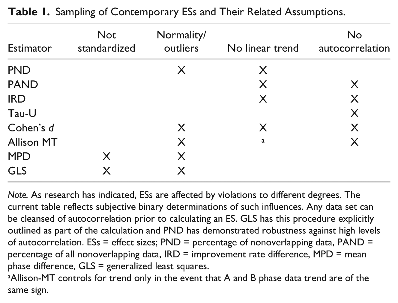
Note. As research has indicated, ESs are affected by violations to different degrees. The current table reflects subjective binary determinations of such influences. Any data set can be cleansed of autocorrelation prior to calculating an ES. GLS has this procedure explicitly outlined as part of the calculation and PND has demonstrated robustness against high levels of autocorrelation. ESs = effect sizes; PND = percentage of nonoverlapping data, PAND = percentage of all nonoverlapping data, IRD = improvement rate difference, MPD = mean phase difference, GLS = generalized least squares.

Allison-MT controls for trend only in the event that A and B phase data trend are of the same sign.

Normality and independence are two common assumptions most researchers are familiar with. Normality is defined as whether the theoretical distribution a sample is drawn from follows the well known “bell-shaped” curve (Cohen, Cohen, West, & Aiken, 2003). Independence in the current study is defined as the degree residuals among adjacent observations are uncorrelated—one observation should convey no information about the next. SCDs consistently violate this assumption due to their within-subject focus. This can result in the presence of trend and autocorrelation. Trend is defined as any systematic pattern within or across phases other than a level shift across conditions. There has been discussion in the literature regarding whether single-case ESs should control for trend, allow trend to contribute to ESs, model trend in isolation, or ignore trend all together, with linear trend nearly always being the focal point (e.g., Parker et al., 2011b). Recently published statistics have included trend parameters (Maggin et al., 2011; Manolov & Solanas, 2013; Parker et al., 2011b).

Autocorrelation, or serial dependency, is defined as the degree of relationship between each datum point and a preceding datum point, most often the immediately preceding observation (Lag 1 autocorrelation). This can be interpreted as how well a time-series data set is explained by a lagged version of itself (Bence, 1995; Huitema & McKean, 1991). Addressing autocorrelation is challenging given the complexity of estimation and cleansing at the individual phase level, especially with lower phase n (Huitema & McKean, 1991). The severity of autocorrelation in SCDs and the need for corrections have been debated thoroughly in the literature (e.g., Bence, 1995; Busk & Marascuilo, 1988; Huitema, 1985; Jones, Weinrott, & Vaught, 1978; Shadish & Sullivan, 2011). Contemporary research has demonstrated that if autocorrelation is present, such fixes are worth considering (Bence, 1995; Levin et al., 2012; Manalov & Sonalas, 2008).

Manolov and Solanas (2008) used Monte Carlo simulations to test the relative merits of five different ESs: percentage of nonoverlapping data (PND), Cohen’s d, Gorsuch’s trend analysis, White et al.’s d, and Allison and Gorman. The authors found that autocorrelation had a general positive linear relationship with ES magnitude with regression-based procedures being the most affected relative to simpler indices (PND, Cohen’s d).

Manolov and Solanas (2012) found that the appropriate use of two recently published SCD ESs—the generalized least squares (GLS) and the mean phase difference (MPD)—was contingent on the properties of the data. Under the specific occurrence of positive baseline autocorrelation and negative intervention phase autocorrelation, GLS was preferable to the MPD. Modeling trend differences were more accurately represented by GLS as well. However, MPD performed well overall, could be calculated more easily, and avoided possible complications in the estimation and cleansing of autocorrelation. The study highlights how knowledge of violations of assumptions can guide the researcher to an appropriate statistic.

To highlight the effects of autocorrelation, Figure 1 recreates data from baseline and intervention of Participant 3 from a math intervention (MI) study authored by McDougall and Brady (1998). Baseline serial dependency was ρ = −.05 (virtually none) and intervention autocorrelation ρ = .44 (severe). Cleansing was applied to the intervention condition, shrinking autocorrelation to −.12. The change shrinks Tau-U by 14%, R² by 10%, and the MPD by 12%, providing an example of why knowledge of the properties of the data is useful in framing the magnitude of the ES. One may also note that the positive autocorrelation leads to visible positive trend in the intervention phase. Indeed, positive autocorrelation and positive trend share data characteristics (Yue, Pilon, Phinney, & Cavadias, 2002), making them correlated in many circumstances.

Figure 1.

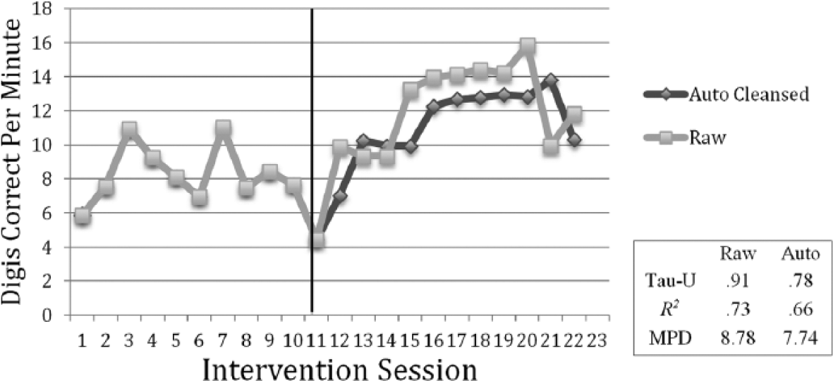
Sample single-case data from McDougall and Brady (1998).

Prior research has suggested that autocorrelation is present in SCDs in low and variable amounts. Shadish and Sullivan (2011), in a large cross-disciplinary sample of SCD studies, calculated a meta-analytic mean of $\bar{r}$ = −.037, with significant heterogeneity across studies. Parker et al. (2011b) estimated that at least one third of extant research had undesirable levels of autocorrelation (r_auto > .20). However, Shadish and Sullivan used a broad convenience sample, which limits findings to specific areas of the field.

In summarizing these assumptions, it is worth noting that autocorrelation and trend are not necessarily problematic from an experimenter’s perspective. Perfect autocorrelation and trend would yield a perfectly stable trend line, stability being a desirable characteristic for many SCD researchers (Kazdin, 1982). Thus, such features are not to be necessarily avoided. Rather, researchers must become knowledgeable about the likelihood of such occurrences, be knowledgeable about the suitable transformations and ESs, and be able to interpret them appropriately given the nature of the data.

SCDs and Meta-Analysis

While widely accepted methods for meta-analysis exist for group-design data, such a framework has yet to emerge for SCD synthesis. A variety of methods have been proposed, involving parametric and nonparametric statistics (e.g., Beretvas & Chung, 2008; Parker & Vannest, 2012; Shadish et al., 2008). Researchers have often attempted to account for this uncertainty by calculating meta-analytic results across different ESs. This procedure constitutes a form of sensitivity analysis (The Cochrane Colloboration, 2012) and—theoretically—allows one to evaluate the robustness of findings by examining the convergence of results calculated using different methods.

If ESs within the same meta-analysis are differentially affected by existing violations stemming from a single data set, this form of sensitivity analysis may no longer be valid because disparate results would be expected. This raises the question as to why one would compare, for example, a nonparametric with a parametric procedure or would expect more generalizable conclusions if two similar nonoverlap procedures are used as opposed to one. If violations of assumptions were moderate to severe, this would have implications for how past and future meta-analyses are interpreted that have used this form of sensitivity analysis.

Current Study

While the extant literature highlights the pitfalls of selecting an ES that is mismatched with violations or interpreted without respect to these violations, it is not known how concerned applied researchers should be. With this in mind, the current study seeks to answer the following questions:

What is the prevalence and severity of violations of normality and independence within the school-based SCD literature?

Are these violations consistent across disciplines or phase types?

If violations were found to be ubiquitous across the literature, this would have significant implications for researchers. While knowledge of such violations does not directly lead to a complimenting ES, an understanding of the context of the data allows more informed choices based on what is known about how certain statistics respond.

It seems unlikely that the same combination of violations would occur consistently across the different applied areas that use SCDs. Therefore, data from four independent domains of school-based research were compared. Phase type (Baseline, Intervention, Maintenance) was also selected as a moderator, as it is possible that trend or nonnormality may be more present in one phase over another. As an example, it may be that baseline phases have higher levels of nonnormality because subjects often show a floor effect on a skill to be learned during intervention.

Method

Sample

Single-case data from three domains within the school-based intervention literature were collected in prior studies. This included populations of studies focused on the application of school-wide positive behavior support (SWPBS), teacher performance feedback (PF) to enhance treatment integrity, and individual math interventions (MI). These data sets were gathered for the purpose of traditional SCD meta-analysis for the former two groups and are described in detail in Solomon, Klein, Hintze, Cressey, and Peller (2012) and Solomon, Klein, and Politylo (2012). The latter group of studies was collected as part of a recent effort to evaluate an outcome efficiency metric for SCD MI’s (Poncy, Solomon, Moore, Simons, & Duhon, 2013). As such, these research syntheses represented the entirety of the peer-reviewed literature within their respective fields at the time of publication. Dependent variables (DVs) for SWPBS included office discipline referrals and various direct measures of student problem behavior. For PF, DVs included completed treatment steps and the frequency of target behaviors (e.g., behavior specific praise). The MI DV was exclusively digits correct per minute.

A fourth data set was gathered specifically for inclusion in this study. This data set focused on the remediation of general education, classroom-based, individual student externalizing problems (Behavior). The application of individual interventions over classwide interventions separates this discipline from SWPBS and there were no shared studies between these two areas. This discipline was chosen because it represented an area of the SCD field that is popular, applicable to school-based interventionists, and was not covered by the other three domains. The search for this pool of studies occurred in the PsychINFO, ERIC, and Academic Search Premier databases in December of 2012 using the search terms “classroom,” and “behavior” and “single subject” or “single case,” yielding 235 and 130 results, respectively. From this pool, a convenience sample of 24 studies was selected, which was the median number of studies for the other three groups. DVs included off-task and on-task student behaviors and correct student responses. The 24 studies selected were the first ones to meet criteria within the search results. Table 2 describes characteristics of each group of studies. Overall, 104 studies were included, which amounted to 1,576 phases of data.

Table 2.

Characteristics of Sample.

Discipline	Date of search^a	No. of studies	Average baseline	Average intervention	Average maintenance	Designs present
SWPBS^b	05-08	20	8.55 (21.76)	11.93 (32.17)	6.78 (8.33)	MBD, AB
PF^c	04-10	36	9.19 (33.07)	9.95 (41.03)	8.67 (24.50)	MBD
Math^d	07-12	24	7.71 (28.25)	8.85 (36.37)	9.96 (32.00)	MBD, AT
Behavior	12-12	24	7.43 (22.08)	8.83 (49.74)	11.64 (32.00)	MBD, AT, Reversal

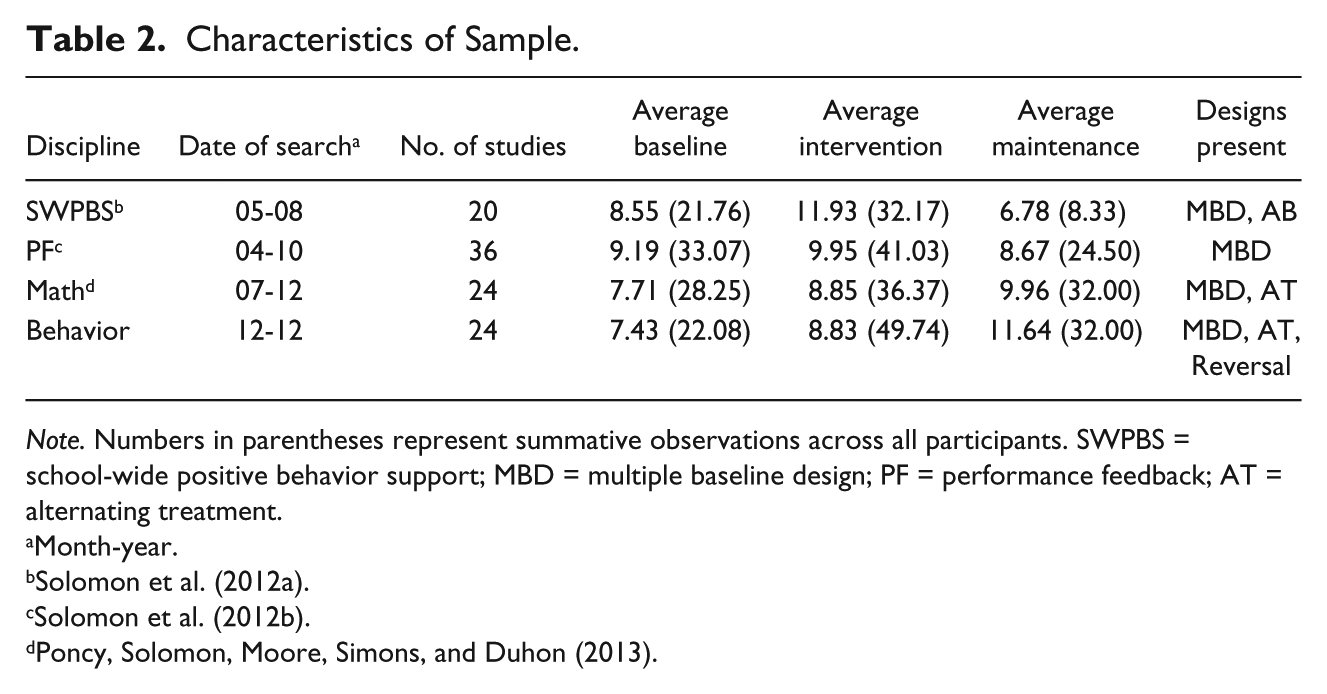
Note. Numbers in parentheses represent summative observations across all participants. SWPBS = school-wide positive behavior support; MBD = multiple baseline design; PF = performance feedback; AT = alternating treatment.

Month-year.

Solomon et al. (2012a).

Solomon et al. (2012b).

Poncy, Solomon, Moore, Simons, and Duhon (2013).

Data Extraction

Single-case articles typically do not present the requisite information required to calculate ESs, autocorrelation, trend, or skew. Fortunately, Parker et al. (2005) outlined procedures for digitizing time-series graphs. Shadish et al. (2009), using a similar procedure with the program UnGraph, reported high reliability and found that the digitized data were a faithful representation of the original observations. All data analyzed in the current study were recreated using this digitizing procedure.

Moderators and DVs

The two moderators evaluated were phase type and discipline. The levels of discipline were previously defined as SWPBS, PF, MI, and Behavior. The levels of phase type were Baseline, Intervention, and Maintenance. These two moderators addressed whether violations occur in greater severity for certain types of populations and for different phases. To evaluate violations of assumptions along these dimensions, measures of autocorrelation, trend, and normality were calculated for each phase of each study. Only phases greater than six datum points were included, as this was the minimum number of points Huitema and McKean (1991) reviewed in their analysis of the effects of small sample bias in the estimation of Lag 1 autocorrelation. This eliminated 31% of individual phases across all studies.

Autocorrelation

Lag 1 serial dependency was measured using a common formula, as reported in Huitema and McKean (1994) and Shadish, Rindskopf, Hedges, and Sullivan (2013):

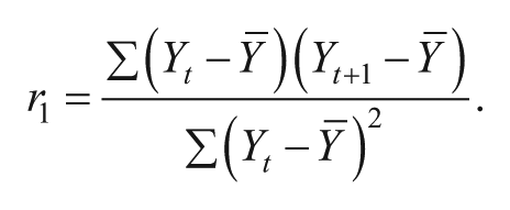
r_{1} = \frac{\sum (Y_{t} - \bar{Y}) (Y_{t + 1} - \bar{Y})}{\sum {(Y_{t} - \bar{Y})}^{2}} .

One may note the similarity to the Pearson’s correlation coefficient, which is how the resulting statistic is interpreted. Raw and absolute values of autocorrelation were calculated, because autocorrelation in either a positive or negative direction poses challenges in the interpretation of ESs. Because the term $Y_{t + 1}$ contains N − 1 datum points less than the original sample, estimation bias is introduced not normally present in the Pearson’s r, which increases in severity as N decreases (Huitema & McKean, 1991, 1994). This bias was reduced in the current study by the application of the random-effects meta-analysis, described below.

Trend

Linear trend can be calculated in a variety of ways, most commonly by regressing the DV onto time. The resulting ordinary least squares (OLS) unstandardized $β_{slope}$ is informative but not comparable across studies, while the standardized $β_{slope}$ loses its context but is comparable across studies. Standardized trend was calculated using a parametric and nonparametric estimator. The parametric estimator was calculated by calculating the relationship between the X-axis DV and time (rescaled as $n = 1, 2, 3, \dots, k$ ), resulting in an r statistic. Monotonic slope was calculated using the Kendall Rank Correlation (KRC) by analyzing overlap within phase, as recommended in Parker et al. (2011b). Monotonic trend measures the tendency for observation points to increase upon prior values but does not measure conformity to a linear regression line. Absolute values were used. Parametric trend was calculated only for those studies that yielded reasonable normality (skew or kurtosis between −2 and 2; 81%), while monotonic trend was calculated for the remaining nonnormal data (19%).

Normality

Normality was evaluated by calculating estimates of skew and kurtosis using the standard values provided by SPSS 20. Absolute values were calculated because excessive skew and kurtosis result in similar accommodations (e.g., nonparametric analysis).

Analysis

Meta-analytic procedures were used to control for sampling error. Procedures outlined by Shadish et al. (2012) for the random-effects meta-analysis of serial dependency were used to calculate weighted autocorrelation values. Trend values were synthesized using a standard random-effects model (Cooper, Hedges, & Valentine, 2009). Monotonic slope was accommodated by converting Kendall τ’s to Pearson r’s using the equation drawn from Kendall (1970), r_τ = sin(.5πτ). Heterogeneity within and across moderators (Q) was measured, which was also converted into a percentage of present heterogeneity (I²; Higgens & Thompson, 2002) to aid interpretation. Due to small sample size for monotonic trend, only the omnibus mean is reported without comparisons within moderators.

Skew and kurtosis were synthesized using a fixed effects meta-analysis (Cooper et al., 2009). Data were doubly weighted so that each article could only contribute up to three ESs: one for Baseline, Intervention, and Maintenance. At the article level, data were weighted by sample size. At the meta-analysis level, studies were weighted by the inverse of their variance, which was corrected for overall sample heterogeneity in the case of random-effects synthesis.

Planned comparisons were conducted using analog ANOVA for the DVs of autocorrelation and parametric trend. This was composed of comparisons of all disciplines (i.e., SWPBS, PF, MI, Behavior) collapsed across phases and between phases (i.e., Baseline, Intervention, Maintenance) collapsed across discipline. The Bonferonni correction was applied to control for multiplicity issues, although this did not invalidate any previously significant findings.

Results

Autocorrelation

Autocorrelation across studies was low and heterogeneous (see Table 3). The overall mean was not significantly different than 0, ${\bar{r}}_{1}$ = .06, 95% confidence interval (CI) = [−.01, .13], although absolute values were greater, ${\bar{r}}_{1}$ = .36, 95% CI = [.32, .41]. Autocorrelation was on average significantly greater than zero for two levels of the included moderators: MI, ${\bar{r}}_{1}$ = .31, 95% CI = [.18, .45] and Intervention phase, ${\bar{r}}_{1}$ = .12, 95% CI = [.02, .22]. Heterogeneity values were always significant, ranging from Q = 43.85 to Q = 2,209.16 with total sample I² of 73%. The parceling of studies into discipline reduced the I² nominally (65%). A histogram of r₁ values (Figure 2) yielded a mildly leptokurtic distribution centered around ${\bar{r}}_{1}$ = 0 with slight positive skew.

Table 3.

Summary of Random-Effects Meta-Analysis of Lag 1 Autocorrelation.

	Q	τ	SE	Lower Limit	M	Upper Limit
SWPBS	339.94* (145.56)*	.23 (.08)	.08 (.06)	−.17 (.20)	−.01 (.31)	.15 (.42)
PF	371.46* (171.28)*	.09 (.02)	.04 (.02)	−.04 (.27)	.04 (.32)	.12 (.36)
Behavior	371.23* (143.28)*	.20 (.06)	.07 (.05)	−.13 (.28)	.01 (.37)	.15 (.46)
Math	292.51* (155.97)*	.12 (.05)	.07 (.05)	.18 (.42)	.31 (.52)	.45 (.62)
Baseline	465.83* (204.85)*	.14 (.14)	.05 (.05)	−.10 (.23)	−.01 (.32)	.08 (.41)
Intervention	1,300.47* (534.29)*	.22 (.21)	.05 (.05)	.02 (.29)	.12 (.39)	.22 (.49)
Maintenance	43.85* (14.96)	.04 (.03)	.06 (.06)	−.04 (.23)	.09 (.34)	.21 (.46)
Total	2,209.16* (804.52)*	.04 (.06)	.04 (.02)	−.01 (.32)	.06 (.36)	.13 (.41)

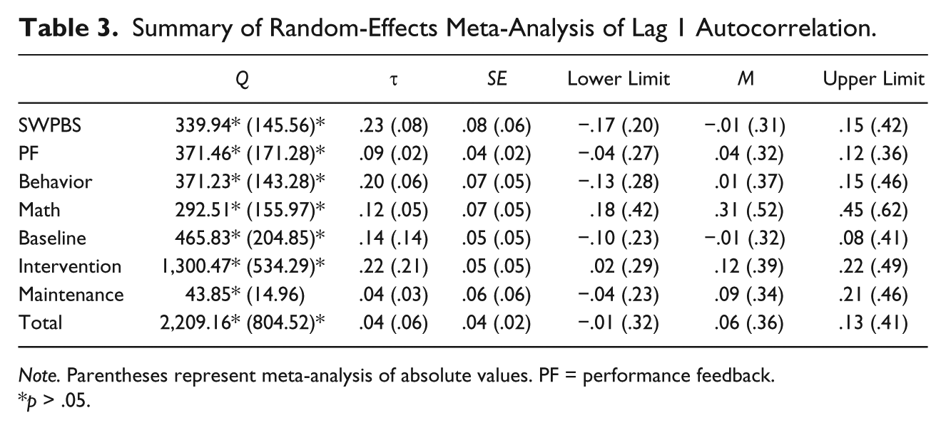
Note. Parentheses represent meta-analysis of absolute values. PF = performance feedback.

p > .05.

Figure 2.

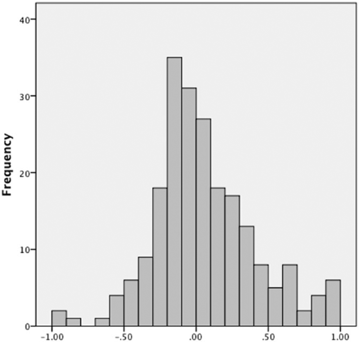
Histogram of phase-level autocorrelation.

Analog ANOVAs (Table 4) resulted in significance for the discipline moderator (Q_b = 15.66, p = .001) but not for phase type. Post hoc analysis yielded significant differences between SWPBS and MI (Q_b = 9.15, p < .01), PF and MI (Q_b = 11.97, p < .01), and Behavior and MI (Q_b = 9.12, p < .01), with MI being greater in all cases.

Table 4.

Analog ANOVAs of Lag 1 Autocorrelation.

	Q_w (df)	Q_b (df)	p
Discipline	127.24 (214)	14.66 (3)	< .01
SWPBS vs. PF	69.57 (133)	0.30	.58
SWPBS vs. Behavior	38.68 (89)	0.64	.42
SWPBS vs. Math	48.74 (78)	9.15	< .01
PF vs. Behavior	78.50 (134)	0.12	.73
PF vs. Math	87.96 (122)	11.97	< .01
Behavior vs. Math	57.68 (80)	9.12	.003
Phase	119.55 (215)	3.84 (2)	.15
Baseline vs. Intervention	—	—	—
Baseline vs. Maintenance	—	—	—
Intervention vs. Maintenance	—	—	—

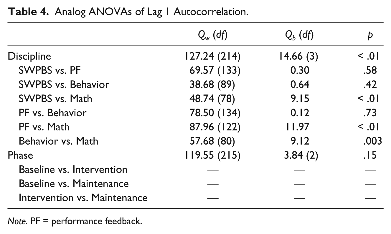
Note. PF = performance feedback.

Trend

Parametric trend values ( ${\bar{r}}_{1}$ ; Table 5) were significant and moderate, ${\bar{r}}_{1}$ = .36, 95% CI = [.28, .43], with high levels of heterogeneity (I² = 80%). Conversion to R² shows that on average, 13% of the variability within phase is explained by trend. MI had notably higher trend than average values, ${\bar{r}}_{1}$ = .70, 95% CI = [.54, .81], while trend within Behavior intervention studies was the lowest, ${\bar{r}}_{1}$ = .21, 95% CI = [.07, .35], and also the most homogeneous, Q = 24.49. Sorting of studies into discipline and phase reduced I² to 63% and 74%, respectively. Only the discipline moderator was significant (Q_b = 19.36, p < .01; Table 6), with follow-up analysis showing that trend in MI studies was significantly higher than all other moderators; 57% of adjacent phase pairs included trend in the same direction.

Table 5.

Summary of Random-Effects Meta-Analysis of Parametric Trend.

	Q	τ	SE	Lower Limit	M	Upper Limit
SWPBS	47.15	0	.08	.18	.33	.46
PF	101.55*	.01	.05	.15	.25	.34
Behavior	24.49	0	.08	.07	.21	.35
Math	297.13*	.29	.14	.54	.70	.81
Baseline	95.92	0	.05	.16	.26	.36
Intervention	698.68*	.22	.08	.31	.44	.55
Maintenance	19.01	0	.11	.07	.28	.47
Total	876.55*	.13	.05	.28	.36	.43

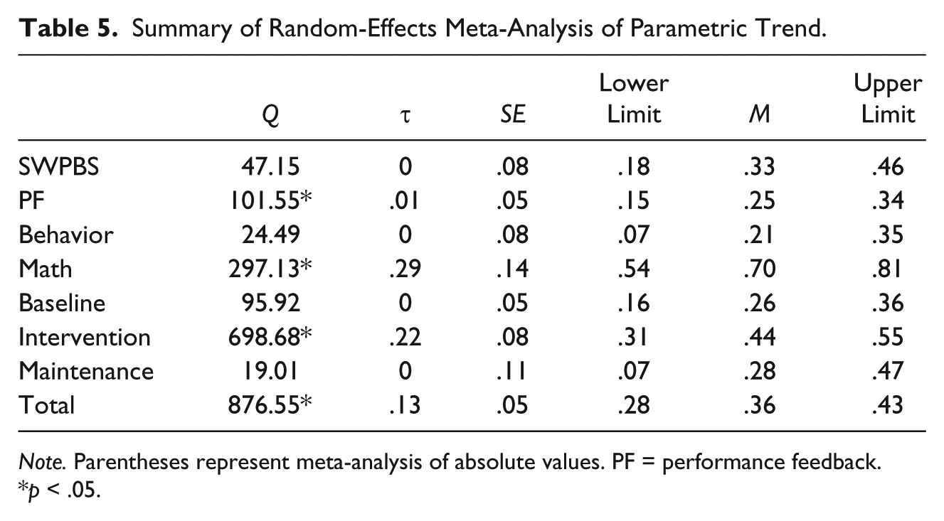
Note. Parentheses represent meta-analysis of absolute values. PF = performance feedback.

p < .05.

Table 6.

Analog ANOVAs of Parametric Trend.

	Q_w (df)	Q_b (df)	p
Discipline	53.72 (214)	19.36 (3)	< .01
SWPBS vs. PF	31.18 (133)	0.36	.55
SWPBS vs. Behavior	20.61 (89)	0.69	.40
SWPBS vs. Math	27.09 (78)	12.29	< .01
PF vs. Behavior	26.63 (134)	0.13	.71
PF vs. Math	33.11 (122)	17.68	< .01
Behavior vs. Math	22.53 (80)	17.35	< .01
Phase	68.52 (175)	4.87 (2)	.09
Baseline vs. Intervention	—	—	—
Baseline vs. Maintenance	—	—	—
Intervention vs. Maintenance	—	—	—

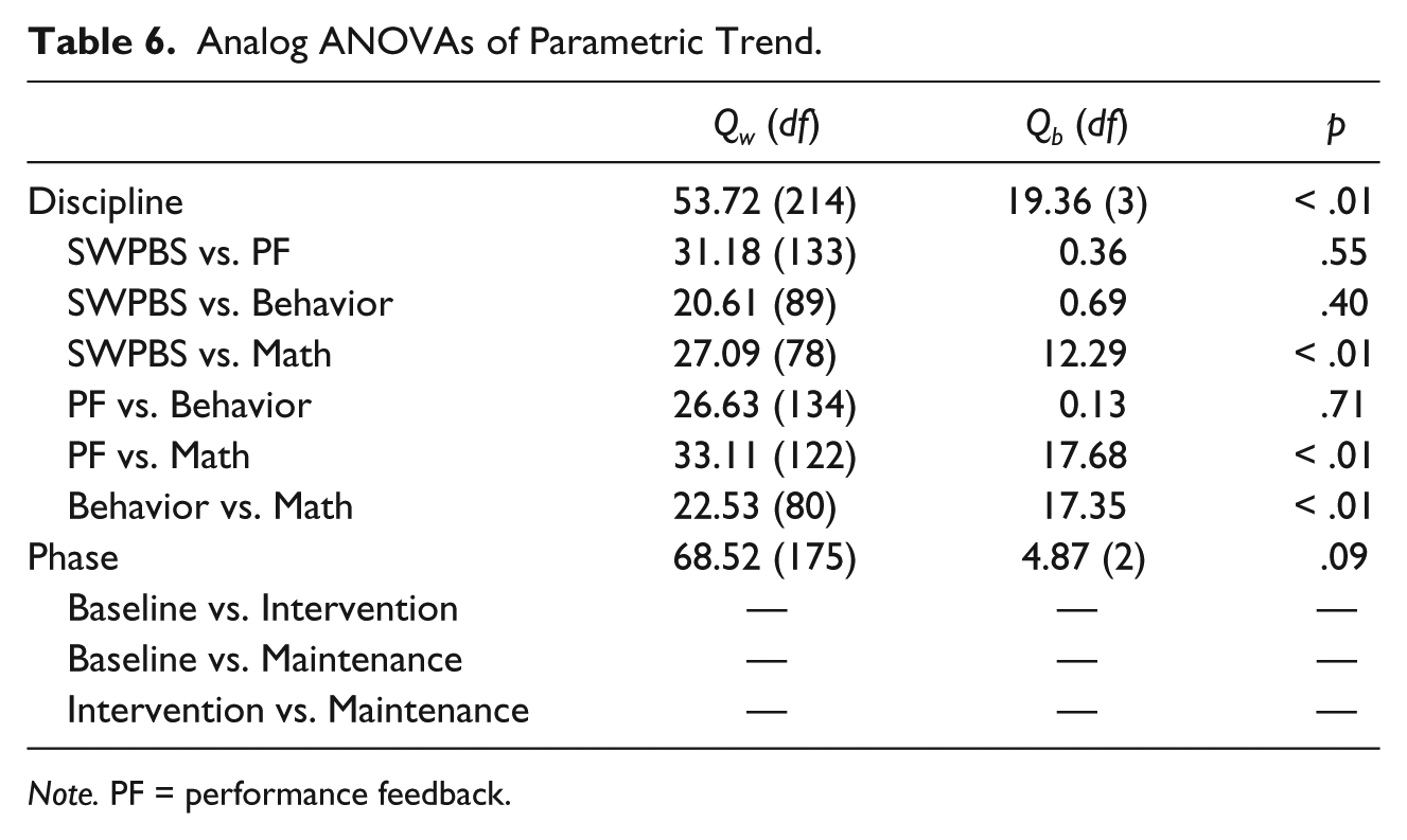
Note. PF = performance feedback.

Given the small number of slopes analyzed using the KRC, only omnibus statistics are reported. Overall heterogeneity was significant, Q = 101.08, p < .01, and I² = 60%. The overall mean was ${\bar{r}}_{m}$ = .31, 95% = [.12, .47], once again suggesting that trend was modest but clearly present.

Skew and Kurtosis

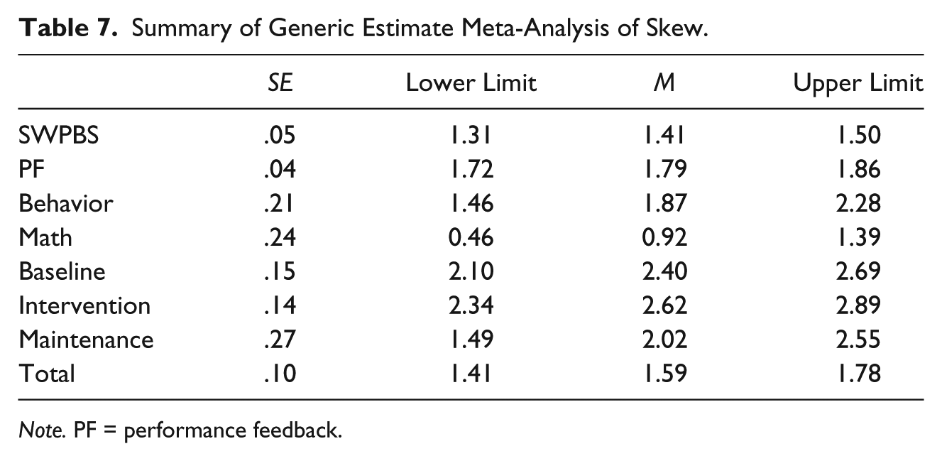
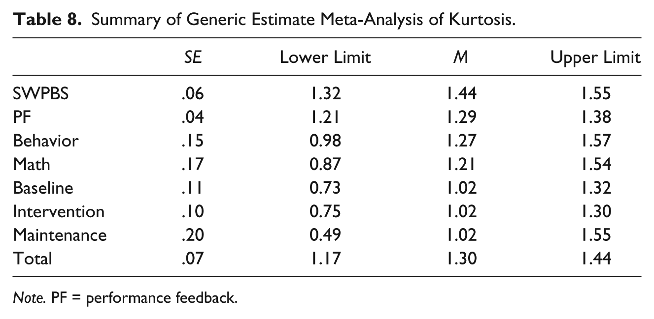
Tables 7 and 8 show that skew and kurtosis were present at significant levels for all levels of both moderators. However, levels were low, typically mild to moderate if values within the range of −2 to 2 are used as a rough benchmark. Inspection of the data showed that only seven study phases, collapsed across studies, yielded skew values outside this range, which represented 3% of included study phases. Thirty-seven study phases (17%) had excessive kurtosis values. Organized by level, Intervention conditions had the highest level of skew and kurtosis means were fairly equal across moderators.

Table 7.

Summary of Generic Estimate Meta-Analysis of Skew.

	SE	Lower Limit	M	Upper Limit
SWPBS	.05	1.31	1.41	1.50
PF	.04	1.72	1.79	1.86
Behavior	.21	1.46	1.87	2.28
Math	.24	0.46	0.92	1.39
Baseline	.15	2.10	2.40	2.69
Intervention	.14	2.34	2.62	2.89
Maintenance	.27	1.49	2.02	2.55
Total	.10	1.41	1.59	1.78

Note. PF = performance feedback.

Table 8.

Summary of Generic Estimate Meta-Analysis of Kurtosis.

	SE	Lower Limit	M	Upper Limit
SWPBS	.06	1.32	1.44	1.55
PF	.04	1.21	1.29	1.38
Behavior	.15	0.98	1.27	1.57
Math	.17	0.87	1.21	1.54
Baseline	.11	0.73	1.02	1.32
Intervention	.10	0.75	1.02	1.30
Maintenance	.20	0.49	1.02	1.55
Total	.07	1.17	1.30	1.44

Note. PF = performance feedback.

Discussion

The purpose of the current study was to investigate the severity of assumption violations within SCDs. A greater knowledge of these patterns may help guide researchers in selecting appropriate ESs and provide additional context for their interpretation. Results demonstrated that low and variable levels of autocorrelation, moderate and significant levels of trend, and relatively normal data patterns emerged across studies. Moderation was present, suggesting that certain types of studies have more severe levels of trend and autocorrelation than others. Overall levels of heterogeneity affirm the need for researchers to review assumption violations in their data. This is a good habit regardless of whether visual analysis, ESs, or both techniques are used.

Autocorrelation

Shadish and Sullivan (2011) found that autocorrelation within a sample of 113 studies was significant; however, the average effect was small and variable. The current study affirms this at the omnibus level. However, studies that focused on MI had more elevated yet inconsistent levels of autocorrelation.

Resulting ESs drawn from this area may need to be taken with a grain of salt; ESs will likely be inflated due to suppressed standard errors and significance tests more generous than their nominal levels. As an example, Manolov and Solanas (2008) found that positive autocorrelation of ρ = .30 inflated the Allison and Gorman R² (a mean + trend procedure) by roughly .09 and inflated the point biserial R² by .04 ( $n_{PhaseA}$ = 5, $n_{PhaseB}$ = 10) beyond nominal levels. Autocorrelation of ρ = .60 inflated these ESs by roughly .16 and .10. Nonparametric alternatives are also affected, although to a lesser degree. Parker et al. (2011b) found that for the upper range of Tau-U values (90th percentile), autocorrelation had a strong influence, although effects were modest below this benchmark. The MPD has demonstrated robustness to autocorrelation, having borrowed the straightforward differencing concept from economics (Manolov & Solanas, 2013), as does its closely related cousin, the slope-and-level change (SLC; Solanas, Manolov, & Onghena, 2010). Naturally, the GLS is well equipped to handle most situations of high serial dependency (Maggin et al., 2011).

Given these results, it can only be stressed that this assumption should be reviewed prior to the calculation of ESs, if anything to provide a more accurate context for the magnitude of effect. High levels of heterogeneity suggest that there is no magic bullet ES, even within discipline. The researcher will need to make an informed choice, recognizing that within any pool of studies, some effects will be more biased than others. To clarify this issue, researchers conducting meta-analysis may want to graph their review of assumptions. Shadish and Sullivan (2011) provided one example of how to graph autocorrelation by study sample size.

It also is worth noting that given the high frequency of phases with small n (<6) in the current sample, reliable cleansing would often not be possible. For the GLS, Maggin et al. (2011) recommended that there be at least 5 datum points per phase and at least 20 total points. Although the authors suggested that points could be summative across participants, the assumption of equal serial dependency comes with this adjustment. A similar issue occurs with trend; the estimation of such trend should be reliable, which is largely a function of baseline n. If trend cannot be reliably estimated, the effect on trend-control ESs can be severe, and level change ESs may be a wiser choice.

Trend

Results indicate that absolute levels of parametric trend were consistently present, with values ranging from small to moderate. MI in particular showed high levels of trend (on average, 49% of explained variability of within-phase data), while trend within behavior interventions studies was fairly modest (4% of explained variability). Levels of nonparametric trend were also elevated, suggesting that this is a concern for studies with nonnormal data as well.

These significant levels of trend pose challenges to researchers and will affect statistical outcomes by increasing decision error. A classic example is in the case of across-phase trend. If a trend extends across phases, as it did in 57% of the current sample, Type I error rates will be elevated for mean difference or overlap procedures. A similar effect occurs for visual analysis in the presence of trend (Mercer & Sterling, 2012). This can be controlled through proper design specification, because phase reversals would expose the phenomena if such reversals are possible. It is worth noting that few meta-analyses have attempted to account for trend. None of the extant MI meta-analyses have done so.

The discussion on how best to model trend is still active, with recommendations, including combining the effects of trend- and mean-level difference (e.g., GLS, Tau-U + Trend, MPD), controlling for trend (e.g., ALLISON-M, Gorsuch’s trend analysis, Tau-U), ignoring the issue (e.g., Cohen’s d, NAP, percentage of all nonoverlapping data [PAND]), or modeling trend and/or level differences separately (Theil-Sen, SLC). The more recent generation of trend-control ESs including the GLS, SLC/MPD, and Tau-U each have their own advantages and disadvantages, but as a whole, pose distinct benefits over their older counterparts.

Normality

Sample data can deviate from expected normality due to small n, outliers, or an underlying nonnormal population of observations. While ceiling and floor effects, which occurred for a number of reviewed graphs, would skew distributions, generally speaking across disciplines and phases data, normality was evenly distributed. This violation was most pronounced for Intervention and then Baseline phases, where data had the greatest tendency to hit minimum or maximum y-axis values. In the event of nonnormality, ignoring other issues, nonparametric procedures such as permutation tests or nonoverlap ESs (e.g., PAND, Tau-U) are well suited.

Summary

Current findings suggest that for most experiments, simple level difference ESs will be calculated in the presence of trend. However, trend estimates varied, and in the situation of low levels of trend or questionable trend, level difference approaches (e.g., improvement rate difference [IRD], Cohen’s d, PAND) are probably the most appropriate. In the majority of cases where trend is present, certainly trend-controlled procedures are called for and should be used far more often then they currently are. These methods also are generally robust to autocorrelation; however, the GLS remains a strong option to handle trend and autocorrelation when its assumptions are met and the researcher possesses the technical ability to calculate it.

Limitations

Autocorrelation was likely underestimated, with increasing negative bias as study N decreased. While corrections for this bias have been proposed (Huitema & McKean, 1991, 1994), this introduces new problems in the synthesizing of data. To combat this issue, random-effects meta-analysis was used and phases with less than six datum points were removed. Research has shown, however, that even with samples of six or more datum points, estimates of autocorrelation can still be suppressed (Huitema & McKean, 1991, 1994), which is a concern for meta-analysis and estimation at the individual study level.

Measurement issues also affect trend in the rescaling of the x-axis time variable. For example, studies that sampled participant behavior once a month would have trend treated in the same way as a study that sampled behavior every hour, despite the fact that different trends might have emerged over the broader time scale. This would complicate meta-analysis as well and is something researchers should be weary of, yet have largely ignored. Various time scales may also be present within a single phase; it is not always that the case observations occur on a perfectly regular schedule. This is a limit of all current trend-control ESs and represents a circumstance where mean-level statistics may be a wiser choice.

The current study only addressed linear trend in the case of the parametric estimates. It is plausible that curvilinear trends exist frequently in SCDs. However, this is more difficult to reliably test for, if not impossible in some cases, given the small within-phase n that was frequently observed. High levels of heterogeneity also limit generalizable conclusions. Although significant differences were noted, the results were not clear enough to absolve researchers of performing their own review of assumptions.

Finally, it is worth reiterating that the current study sheds light on the context of ES selection and interpretation, but results do not lead to clear links between specific data sets, chosen ESs, and the degree of over- or underestimation of effects. These relationships change based on a number factors, one of which is the constantly evolving literature on the nature of these relatively new parameters.

Conclusion

The purpose of the current study was to investigate the severity of some common violations of assumptions in the SCD literature. Converging with extant research, it was found that autocorrelation exists in small to moderate amounts for certain groups of studies and varies significantly. Trend was more pronounced, although was heterogeneous for two levels of the moderators, while normality violations occurred at fairly modest levels. Moderator analysis explained significant yet small amounts of heterogeneity in the sample.

Given these results, the accommodation of autocorrelation and trend must be decided on a study by study basis and may inflate Type I error rates for MI studies or closely related disciplines in particular. These parameters were significant enough that trend-control ESs should be considered far more often than they currently are. Given that single-case methods, as opposed to group-design analysis, are intended to be used as much in applied practice as in research, a variety of ESs, ranging in complexity as a function of precision, may be required. Within a research context, an investigation of assumptions is always highly encouraged and will be crucial in informing the best practice in analysis.

Footnotes

Declaration of Conflicting Interests

The author(s) declared no potential conflicts of interest with respect to the research, authorship, and/or publication of this article.

Funding

The author(s) received no financial support for the research, authorship, and/or publication of this article.

Author Biography

Benjamin George Solomon, PhD, is an assistant professor of school psychology at Oklahoma State University. His research interests include evidence-based behavioral prevention, single-case data analysis, and the measurement of effective teaching behaviors.

References

Bence

J. R.

(1995). Analysis of short time series: Correcting for autocorrelation. Ecology, 76, 628-639.

Beretvas

S. N.

Chung

(2008). A review of meta-analyses of single-subject experimental designs: Methodological issues and practice. Evidence Based Communication Assessment and Intervention, 2, 129-141. doi:10.1080/17489530802446302

Busk

P. L.

Marascuilo

L. A.

(1988). Autocorrelation in single-subject research: A counterargument to the myth of no autocorrelation. Behavioral Assessment, 10, 229-242.

The Cochrane Collaboration. (2012). Sensitivity analysis. Retrieved from http://www.cochrane-net.org/openlearning/html/mod14-2.htm

Cohen

West

S. G.

Aiken

L. S.

(2003). Applied multiple regression/correlation analysis for the behavioral sciences (3rd ed.). Mahwah, NJ: Lawrence Erlbaum.

Cooper

Hedges

L. V.

Valentine

J. C.

(2009). The handbook of research synthesis and meta-analysis. New York, NY: Russell Sage Foundation.

Franklin

R. D.

Allison

D. B.

Gorman

B. S.

(1997). Design and analysis of single-case research. Mahwah, NJ: Lawrence Erlbaum.

Higgens

J. P.

Thompson

S. G.

(2002). Quantifying heterogeneity in meta-analysis. Statistics in Medicine, 21, 1539-1558. doi:10.1002/sim.1886

Huitema

B. E.

(1985). Autocorrelation in applied behavior analysis: A myth. Behavioral Assessment, 7, 107-118.

10.

Huitema

B. E.

McKean

J. W.

(1991). Autocorrelation estimation and inference with small samples. Psychology Bulletin, 110, 291-304.

11.

Huitema

B. E.

McKean

J. W.

(1994). Two reduced-bias autocorrelation estimators: rF1 and rF2. Perceptual & Motor Skills, 78, 323-330.

12.

Individuals With Disabilities Education Improvement Act, 20 U.S.C. § 1400 (2004).

13.

Jones

R. R.

Weinrott

M. R.

Vaught

R. S.

(1978). Effects of serial dependency on the agreement between visual and statistical inference. Journal of Applied Behavior Analysis, 11, 277-283.

14.

Kazdin

A. E.

(1982). Single-case research designs: Methods for clinical and applied settings. New York, NY: Oxford University Press.

15.

Kendall

M. G.

(1970). Rank correlation methods (4th ed.). London, England: Charles Griffin & Co.

16.

Levin

J. R.

Ferron

J. M.

Kratochwill

T. R.

(2012). Nonparametric statistical tests for single-case systematic and randomized ABAB . . . AB and alternating treatment intervention designs: New developments, new directions. Journal of School Psychology, 50, 599-624. doi:10.1016/j.jsp.2012.05.001

17.

Maggin

D. M.

Swaminathan

Rogers

H. J.

O’Keefe

B. V.

Sugai

Horner

R. H.

(2011). A generalized least squares regression approach for computing effect sizes in single-case research: Application examples. Journal of School Psychology, 49, 301-321. doi:10.1016/j.jsp.2011.03.044

18.

Manolov

Solanas

(2008). Comparing N = 1 effect size indices in presence of autocorrelation. Behavior Modification, 32, 860-875. doi:10.1177/0145445508318866

19.

Manolov

Solanas

(2013). A comparison of mean phase difference and generalized least squares for analyzing single-case data. Journal of School Psychology, 51, 201-215. doi:http://dx.doi.org/10.1016/j/jsp.2012.12.005

20.

McDougall

Brady

M. P.

(1998). Initiating and fading self-management interventions to increase math fluency in general education classes. Exceptional Children, 64(2), 151-166.

21.

Mercer

S. H.

Sterling

H. E.

(2012). The impact of baseline trend control on visual analysis of single-case data. Journal of School Psychology, 50, 403-419. doi:10.1016/j.jsp.2011.11.004

22.

No Child Left Behind Act of 2001 (January 8, 2002). Pub. L. No. 107-110. 107th Congress.

23.

Parker

R. I.

Brossart

D. F.

(2003). Evaluating single-case data: A comparison of seven statistical methods. Behavior Therapy, 34, 189-211.

24.

Parker

R. I.

Brossart

D. F.

Vannest

K. J.

Long

J. R.

De-Alba

R. G.

Baugh

F. G.

(2005). Effect sizes in single case research: How large is large? School Psychology Review, 34, 116-132.

25.

Parker

R. I.

Vannest

K. J.

(2012). Bottom-up analysis of single-case research designs. Journal of Behavioral Education, 21, 254-265. doi:10.1007/s10864-012-9153-1

26.

Parker

R. I.

Vannest

K. J.

Davis

J. L.

(2011a). Effect sizes in single-case research: A review of nine non-overlap techniques. Behavior Modification, 35, 303-322.

27.

Parker

R. I.

Vannest

K. J.

Davis

J. L.

Sauber

S. B.

(2011b). Combining nonoverlap and trend for single-case research: Tau-U. Behavior Therapy, 42, 284-299. doi:10.1177/0145445511399147

28.

Poncy

B. C.

Solomon

B. G.

Moore

K. E.

Simons

Duhon

G. J.

(2013). Using learning rate and curricular scope to refine the measurement of math-fact intervention outcomes. Manuscript in preperation.

29.

Shadish

W. R.

Brasil

I. C.

Ilingworth

D. A.

White

K. D.

Galindo

Nagler

E. D.

Rindskopf

D. M.

(2009). Using UnGraph to extract data from image files: Verification of reliability and validity. Behavior Research Methods, 4, 177-183. doi:10.3758/BRM.41.1.177

30.

Shadish

W. R.

Rindskopf

D. M.

Hedges

L. V.

(2008). The state of the science in the meta-analysis of single-case experimental designs. Evidence-Based Communication Assessment and Intervention, 2, 188-196. doi:10.1080/17489530802581603

31.

Shadish

W. R.

Rindskopf

D. M.

Hedges

L. V.

Sullivan

K. J.

(2013). Bayesian estimates of autocorrelation in single-case designs. Behavior Research Methods, 45, 813-821. doi:10.3758/s13428-012-0282-1

32.

Shadish

W. R.

Sullivan

K. J.

(2011). Characteristics of single-case designs used to assess intervention effects in 2008. Behavior Research Methods, 43, 971-980. doi:10.3758/s13428011-0111-y

33.

Solanas

Manolov

Onghena

(2010). Estimating slope and level change in N = 1 designs. Behavior Modification, 34(3), 195-218. doi: 10.1177/0145445510363306

34.

Solomon

B. G.

Klein

S. A.

Hintze

J. M.

Cressey

J. M.

Peller

S. L.

(2012a). A meta-analysis of school-wide positive behavior support: An exploratory study using single-case synthesis. Psychology in the Schools, 49, 105-121. doi:10.1002/pits.20625

35.

Solomon

B. G.

Klein

S. A.

Politylo

B. C.

(2012b). The effect of performance feedback on teachers’ treatment integrity: A meta-analysis of the single-case literature. School Psychology Review, 41, 160-175.

36.

Yue

Pilon

Phinney

Cavadias

(2002). The influence of autocorrelation on the ability to detect trend in hydrological series. Hydrological Processes, 16, 1807-1829. doi:10.1002/hyp.1095