A Two-Parameter Logistic Extension Model: An Efficient Variant of the Three-Parameter Logistic Model

Abstract

A three-parameter logistic (3PL) model variant, named the two-parameter logistic extension (2PLE) model, was developed. This new model employs a function that integrates item features according to an examinee’s ability level instead of a fixed guessing parameter used in the 3PL model to quantify guessing behavior. Correct response probabilities from a solution behavior and guessing behavior increase as the level of ability increases. At extreme cases in which the level of ability is close to negative infinity, the 2PLE model degenerates into a 3PL model with a guessing probability at chance level (i.e., 1/m, where m is the number of options). The properties of the 2PLE model were described and compared with those of other guessing models. Then, a simulation study comparing the performance of the 2PLE model with that of the 3PL model under three scenarios was conducted. Results showed that the 2PLE model generally outperforms the 3PL model. Finally, the application of the new model in comparison with several existing models was demonstrated by using two real data sets.

Keywords

three-parameter logistic model guessing parameter two-parameter logistic extension model

Introduction and Motivation

Multiple-choice items are extensively used in standardized tests. Thus, assuming that respondents guess when they are in doubt of the correct response is reasonable (San Martín, del Pino, & de Boeck, 2006). The most popular item response theory (IRT) model that includes guessing is the three-parameter logistic (3PL) model (Birnbaum, 1968), which has been discussed in many papers and books (e.g., Baker & Kim, 2004; Hambleton, Swaminathan, & Rogers, 1991; Han, 2012; van der Linden & Hambleton, 1997; von Davier, 2009). However, several past studies revealed that the 3PL model has technical and theoretical limitations. Moreover, item parameters are often estimated poorly in small numbers of items and respondents (Swaminathan & Gifford, 1979), and guessing parameter is not dependent on a person’s latent trait level.

The aim of the present study is to propose a 3PL model variant including a guessing component that depends on ability levels and item characteristics. First, the authors start by briefly reviewing the viewpoints in the studies of San Martín et al. (2006) and van der Maas, Molenaar, Maris, Kievit, and Borsboom (2011), which motivates the current research. Second, they summarize various existing models that quantify guessing behavior. These models form the prototype of the new model. Third, a new integrated model is introduced followed by a discussion of model properties. Fourth, a series of simulation studies are presented. Finally, two real data examples are described.

Alternative Models With Guessing

In conventional IRT models, the probability of a correct item response depends on the characteristics of items and respondents. For instance, in the popular two-parameter logistic (2PL) model (Birnbaum, 1968), the probability of a correct response $Φ_{i}$ is in the form of

Φ_{i} \equiv Φ (a_{i} (θ - b_{i})) = \frac{1}{1 + \exp (- a_{i} (θ - b_{i}))},

(1)

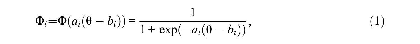
where $a_{i}$ is the item discrimination parameter, and $b_{i}$ is the item difficulty parameter with $i = 1, \dots, I$ indexing items. The examinee subscript is omitted for simplifying the notation throughout the article.

The 2PL model is widely used because it is more flexible than the one-parameter logistic (1PL) model (Rasch, 1960), in which all a_i’s are equal (a_i = 1), although it still provides a relatively parsimonious representation of the association structure in the data. The 2PL model identifies the correct response probability primarily from the solution behavior. Although the 2PL model, similar to other psychometric models, focuses on the representation of individual differences, Tuerlinckx and De Boeck (2005) showed the equivalence between the 2PL model and the diffusion process model for two-choice responses. Their conclusion was further extended in the study of van der Maas et al. (2011). According to the equivalence findings, the 2PL model is somewhat related to the response process models, and the 2PL model can reflect a response process indirectly to some extent. However, the 2PL model only models the successful problem-solving process, and it does not include guessing strategy. Thus, the item characteristic curve (ICC) of the 2PL model has an asymptote of zero. Multiple new models based on the 2PL model have been introduced for solving the guessing problem.

Models With Guessing

Guessing is generally accommodated in IRT through (a) single-process models, such as the Q-diffusion model (van der Maas et al., 2011) and the three-parameter residual heteroscedasticity (3P-RH) model (Lee & Bolt, 2018) and (b) two-process models, which decouple the p process of searching for a correct answer and the g process for guessing (San Martín et al., 2006). One example of the two-process model is the 3PL model. This two-process interpretation, although attractive, does not include other possible serial or parallel processes, and thus single-process models are preferred when the p process and g process are mixed up.

In the two-process model, $p (g)$ quantifies the probability of a correct guess for the g process, and $p (r)$ quantifies the correct response from a solution behavior for the p process. San Martín et al. (2006) formulated a structure of an item response function with a guessing component shown as follows:

P (θ) = p (g) + (1 - p (g)) p (r),

(2)

which can also be rewritten as

P (θ) = p (r) + (1 - p (r)) p (g) .

(3)

The second term, $(1 - p (r)) p (g)$ , is called the guessing part (or guessing component) because it is the term with the guessing component $p (g)$ .

San Martín et al. (2006) argued that three arrangements are possible for the execution of the two processes. In the first one, the g process comes first, and the p process is executed when the g process fails. This arrangement is reflected in Equation 2. That is, a person first makes a guess with a success probability of $p (g)$ . When the guessing fails, the person starts to work on solving the item with a success probability of $p (r)$ . In the second interpretation, the p process comes first, and the g process flows are reflected in Equation 3. In the third one, both processes are executed. When both the g process and the p process fail, a person also fails to answer an item correctly, and this failure results in a correct probability of $1 - (1 - p (r)) (1 - p (g))$ , where $(1 - p (r)) (1 - p (g))$ is the joint probability of incorrectly guessing and solving an item. The resulting correct response probability is exactly the same as those in Equations 2 and 3.

Several models that vary the specific forms of the guessing function $p (g)$ have been proposed. The guessing function $p (g)$ can be a constant, depending on the item characteristics, and the guessing function reduces to a guessing parameter such that $p (g) = c_{i}$ . In this case, Equation 2 becomes the 3PL model when $p (r)$ = $Φ_{i}$ .

Pelton (2002) found that the parameter recovery accuracy for the 3PL model depends on the amount of guessing present in the data. Thus, the estimation of the guessing parameters is unstable. In fact, even when the converged estimates are obtained successfully, the standard errors (SE) of c_i parameter estimates are extremely large to be practical when the sample size is small (<2,000) or when the response matrix is moderately sparse (missing proportion >50%; Han, 2012). As Holland (1990) alluded, the fundamental reason may be that a one-dimensional test can support only two parameters per item. Roughly speaking, as the number of model parameters increases, the number of data points per parameter decreases, and this decrease may cause severe instability (San Martín et al., 2006). Therefore, reducing the number of parameters is considered.

When $a_{i} = 1$ , $Φ_{i}$ degenerates to the 1PL model, and the 3PL model degenerates to the following one-parameter logistic guessing (1PL-G) model:

P_{i} (θ) = c_{i} + (1 - c_{i}) \frac{1}{1 + \exp (- (θ - b_{i}))} .

(4)

Maris (2002) noted that the 1PL-G model and the 3PL model are both not identifiable.

San Martín et al. (2006) suggested that the 3PL model can be used only for large samples unless the guessing parameters are equal to a known or unknown constant. Birnbaum (1968) conjectured that low-ability subjects select a correct response by chance such that the guessing parameter is the same as the chance level $1 / m$ , where m is the number of response options in a multiple-choice item. This conjecture gives rise to the second variation of the 3PL model, which is the 3PL model with a fixed lower asymptote (designated 3PL with FLA). The corresponding item response function has the following form:

P_{i} (θ) = \frac{1}{m} + (1 - \frac{1}{m}) Φ_{i} .

(5)

The 3PL with FLA model has a fixed asymptotic of $1 / m$ that does not relate to ability. The guessing function $p (g)$ is fixed for all items that have the same number of options. Han (2012) showed that the parameter estimation of the 3PL with FLA model is more accurate than that of the 3PL model. However, it is challenging to explain the g process when the guessing parameters of all items are the same.

Pelton (2002) described another limitation of the 3PL model. The calibration of guessing parameters on the basis of the capable and weak samples of respondents may produce substantially different item parameter estimates. Thus, presuming that the success of guessing depends on ability level in some cases is reasonable. Based on this idea, a function $p (g) = λ (θ, δ)$ is proposed, where $δ$ denotes the vector of item parameters. Thus, Equation 2 is rewritten as

P (θ) = λ (θ, δ) + (1 - λ (θ, δ)) p (r) .

(6)

Based on Equation 6, San Martín et al. (2006) proposed a model called the one-parameter logistic ability-based guessing (1PL-AG) model. The success probability of guessing in the 1PL-AG model is defined as

λ (θ, δ) = \frac{1}{1 + \exp (α θ + γ_{i})},

(7)

whereas the success of solution behavior still follows 2PL, that is, $p (r) = Φ_{i}$ . In Equation 7, $α$ is a scaling constant that reflects the dependency of guessing on $θ$ and $γ_{i}$ is the easiness of the guessing process.

The lower asymptote in the 1PL-AG model is zero, which may not hold for multiple choice items because for these items, the worst case that a respondent can do is guess at random. That is, he or she approaches the guessing probability of chance level rather than zero (van der Maas et al., 2011). This situation is one of the main points of the Q-diffusion model, and this axiomatic property continues to hold in our proposed model.

Motivation of the New Model

The motivation for the new model is twofold. First, empirical evidence shows that the average estimated c_i-parameter in the 3PL model is close to 1/m (Han, 2012). As a result, the assumption that low-ability examinees are attracted to incorrect responses is unsubstantiated. Therefore, in theory, the lower asymptote of an ICC should be close to 1/m, which is the success probability of a completely random guessing process.

Second, the success of “educated” guessing depends on an examinee’s ability (San Martín et al., 2006; van der Maas et al., 2011). This ability-based guessing process happens when an examinee guesses an answer from the remaining items after eliminating wrong items. In fact, “almost all formula-scoring instructions in use today, while advising avoidance of completely blind guessing, do encourage examinees to guess whenever they can eliminate a wrong choice” (Frary, 1988, p. 34).

Therefore, it is rational to assume that the probability of a correct guess is 1/m when $θ = - \infty$ , and the correct guessing probability increases when θ increases. Below, a two-parameter logistic extension (2PLE) model that satisfies these characteristics is proposed.

The 2PLE Model

Formulation of the Guessing Function, $p (g) \equiv λ (θ, δ)$

For item i with m_i options, assume that the guessing function relates only to the item parameters (m_i, a_i, b_i) and θ. In the 2PL model, the probability of an incorrect response is

1 - Φ_{i} = \frac{1}{1 + \exp (a_{i} (θ - b_{i}))} .

(8)

Because it is reasonable to assume that a high probability of guessing an item right corresponds to a low possibility of an incorrect response, the correct guessing probability p(g) should have a monotonically decreasing relationship with $1 - Φ_{i}$ . Therefore, the authors suggest,

1 - Φ_{i} = \log_{\frac{1}{m_{i}}} p (g) .

(9)

Equation 9 can be rewritten as

p (g) = {(\frac{1}{m_{i}})}^{\frac{1}{1 + \exp (a_{i} (θ - b_{i}))}} .

(10)

Here, note that this guessing function (Equation 10) integrates the information from both ability levels and item characteristics, and it is called as integrated guessing (IG) function, which is denoted as $p (g) \equiv λ_{i}$ . The IG function is a monotonically increasing function that has the range $1 / m_{i} \leq λ_{i} \leq 1$ for $- \infty \leq θ \leq + \infty$ . In the IG function, the “guessing process” relates to the features of items $(m_{i}, a_{i}, b_{i})$ and the examinee’s ability. If the examinee’s ability is $- \infty$ , then he or she guesses at random, and the probability of he or she guessing correctly is $1 / m_{i}$ .

Notably, our proposed model based on this IG function preserves some axiomatic properties of the 2PL model (such as identifiability and linear invariance). Next, the authors focus on exploring these properties in detail.

Formulation of the Model

By plugging the guessing function into Equation 6 and replacing the success solution probability by the 2PL model, the item response function of the new model has the following form:

P_{i} \equiv P_{i} (θ) = λ_{i} + (1 - λ_{i}) Φ_{i} .

(11)

Note that the 3PL model can be viewed as a special case of this equation by replacing $λ_{i}$ with c_i. In contrast to the 3PL model, this model has only two parameters. Therefore, it is called the 2PLE model. The 2PLE model can actually be viewed as a single-process model because it allows a natural transition from accurate responding to guessing. Having one less parameter to estimate per item typically simplifies the corresponding estimation procedure. The 2PLE model is expected to perform better than the 3PL model because the latter might be overparameterized (Han, 2012; Holland, 1990).

The 2PLE model maintains the monotonicity feature of the original 3PL model in which the correct response probability monotonically increases with increasing $θ$ . This probability lies in the range of $1 / m_{i} \leq P_{i} \leq 1$ for $- \infty \leq θ \leq + \infty$ . When $θ = - \infty$ , $λ_{i} = 1 / m_{i}$ . In this case, the 2PLE model degenerates into the 3PL model with a guessing probability of $1 / m_{i}$ .

In the 2PLE model, when $θ = - \infty$ , the examinee is incapable of obtaining any valuable information from the item options and thus likely to answer questions in a completely random manner. As a result, the probability of a correct response is equal to the chance level $1 / m_{i}$ . Small negative values of $θ$ indicate that the examinee obtains little information from the item but $p (r)$ and $p (g)$ still improve. When $θ = + \infty$ , the probability of a correct response is equal to 1. This new model is particularly suitable for common situations in which an examinee can rule out one or more incorrect response options. Here, an item from the Second School Admission Test (SSAT) is taken as an example.

The average of three numbers is V. If one of the numbers is Z, and another is Y, what is the remaining number?

(A) ZY - V; (B) Z / V - 3 - Y; (C) Z / 3 - V - Y; (D) 3 V - Z - Y; (E) V - Z - Y .

Three numbers are provided, as well as their average. Thus, options (A) and (E) without 3 may be wrong. Some examinees can eliminate one or two response options by using their logical ability.

Identifiability of the 2PLE Model

The 2PLE model is identified with the following restriction: $(a_{1}, b_{1}) = (1, 0)$ . This restriction is the same as the identification restriction of the usual 2PL model. In fact, the 2PLE model can be written as

P_{i} = {m_{i}}^{- (1 - Φ_{i})} + [1 - {m_{i}}^{- (1 - Φ_{i})}] Φ_{i} .

(12)

Here, $P_{i}$ is a monotonically increasing function of Φ_i because the first derivative of $P_{i}$ with respect to Φ_i is nonnegative, that is,

\begin{matrix} P'_{i} = ({m_{i}}^{- (1 - Φ_{i})})' + [1 - {m_{i}}^{- (1 - Φ_{i})}]' Φ_{i} + [1 - {m_{i}}^{- (1 - Φ_{i})}] {Φ'}_{i} \\ = {m_{i}}^{Φ_{i} - 1} \ln m_{i} - Φ_{i} {m_{i}}^{Φ_{i} - 1} \ln m_{i} + [1 - {m_{i}}^{- (1 - Φ_{i})}] \\ = {m_{i}}^{Φ_{i} - 1} (1 - Φ_{i}) \ln m_{i} + [1 - {m_{i}}^{- (1 - Φ_{i})}], \end{matrix}

when $0 \leq Φ_{i} \leq 1, m_{i} > 1, P'_{i} > 0 .$

Also because Φ_i is a monotonic function of θ, the ICC of the 2PLE model is monotonically increasing as a function of θ. Therefore, $P_{i}$ has a one-to-one correspondence with Φ_i, and the identification of the 2PLE model depends on the identification of the 2PL model. The 2PL model is identified when $(a_{1}, b_{1}) = (1, 0)$ (San Martín, Gonzáles, & Tuerlinckx, 2015), and under the same restriction as the 2PL model. The 2PLE model shares the same linear invariance of item parameters with the 2PL model for the same reason. As a result, the linking and scaling methods appropriate for 2PL can also apply for the 2PLE model.

Interpretation of the Model Parameters

The interpretation of item parameters in the 2PLE model is similar to that in the 3PL model. This statement can be verified by applying the idea of Lord and Novick (1968).

In the 2PLE model, when $θ = b_{i}$ ,

P_{i} = λ_{i} + (1 - λ_{i}) Φ_{i} = 0.5 + 0.5 \times constant .

(13)

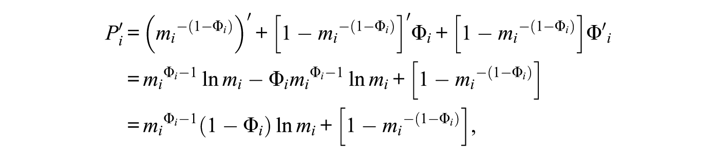
Therefore, $b_{i}$ is still the difficulty parameter, as in the original 3PL model.

For the 2PLE model, taking the first-order partial derivative of $P_{i}$ with respect to $θ$ yields

\frac{\partial P_{i}}{\partial θ} = \frac{\partial Φ_{i}}{\partial θ} [λ_{i} \log (\frac{Φ_{i} - 1}{m_{i}}) + 1 - λ_{i}] .

(14)

In particular, when $θ = b_{i}$ ,

\frac{\partial P_{i}}{\partial θ} = a_{i} \times constant .

(15)

At point b_i, the ICC of the 2PLE model has a slope that is a function of a_i. The slope of the tangent line of the ICC at b_i is proportional to the magnitude of a_i. Thus, from a geometric perspective, a_i can be viewed as the discrimination parameter.

The meaning of the ability parameter is similar to that in the 1PL-AG model, and the ability level not only plays a crucial role in the problem-solving process that is captured in the original 2PL model but also influences the guessing process.

Rationality of the 2PLE Model

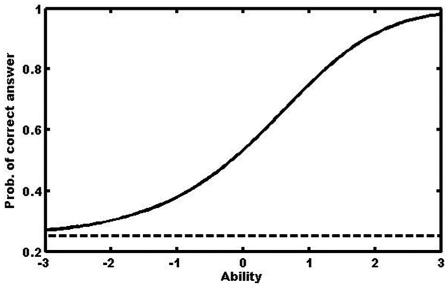
For item i, the lower asymptotic line of the ICC of the 2PLE model is equal to $1 / m_{i}$ . The ICC of item i under the 2PLE model is shown in Figure 1.

Figure 1.

The 2PLE model where a_i = 1, b_i = 1, and m_i = 4.

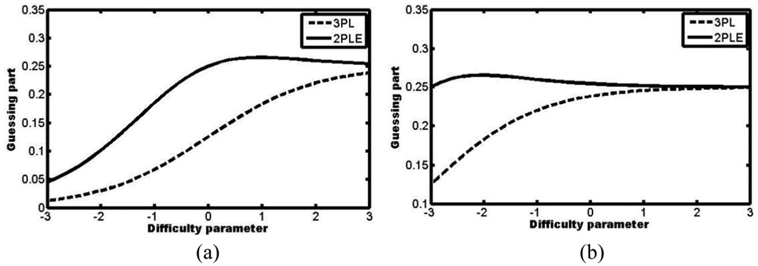
Note that for small negative ability values (e.g., $θ = - 3$ ), a small distance remains between the ICC and the asymptotic line because the examinee’s ability still exists even if it has a small contribution to the guessing probability. This situation is identical to that in the 3PL model, in which the guessing probability is slightly different from the chance level.

The guessing part of the 2PLE model

λ_{i} (1 - Φ_{i})

(16)

is illustrated in Figure 2a and 2b, which present how the guessing component changes as a function of θ. The contribution of the guessing part in the 2PLE model to the probability of success is a single-peaked function of θ. The probability of guessing an item correctly reaches maximum value near the point of $θ = b_{i}$ in the 2PLE model. An examinee likely guesses an item correctly when his or her ability matches the item’s difficulty parameter. To the left of this peak point, the correct guessing probability increases with the increase in ability. Once the ability level exceeds this peak point, the correct guessing probability starts to decrease because the examinees start to answer the item via solution behavior (i.e., based on their ability). By contrast, the correct guessing probability in the 3PL model is a monotonically decreasing function. The probability of guessing correctly has its maximum value when $θ = - \infty$ in the 3PL model and contradicts the phenomenon that the probability of guessing correctly increases in examinees with intermediate ability levels.

Figure 2.

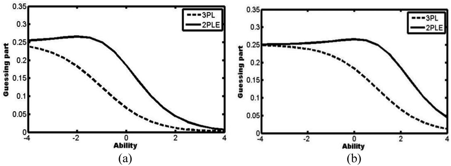
Guessing part (i.e., the second term in Equation 3) of the two models for two items as a function of θ.

Figure 3 illustrates how the guessing part changes as a function of b_i for a fixed θ level. The guessing part in the 2PLE model is a single-peaked function of b_i with the maximum value near the point $b_{i} = θ$ . It implies from Figure 3a that as the item becomes more difficult, the chance of guessing an item correctly increases because solving it correctly may be harder. However, after the peak point, the probability of guessing correctly drops slightly and it stabilizes around 0.25. Similar pattern also exhibits in Figure 3b. On the contrary, the correct guessing probability from the 3PL model keeps increasing as items become more difficult, and this is counterintuitive because it is hard to explain why a person may more likely to guess a difficult item correctly.

Figure 3.

Guessing part of the two models for two fixed θ levels as a function of item difficulty.

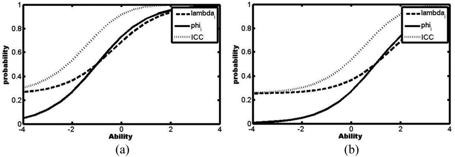
Finally, because the problem-solving process and the guessing process in the 2PLE model share the same set of item parameters (i.e., $a_{i}, b_{i}$ ), it is interesting to illustrate the dependency of these two processes within a given item, as shown in Figure 4. In an item in Figure 4, as ability level increases from –3, the contribution of guessing process increases, and the probability of guessing it correctly dominates the probability of solving an item correctly until the ability matches the item difficulty. When the ability of an examinee exceeds the item difficulty, the probability of solving an item correctly dominates the probability of guessing it correctly. That is, the examinee solves the item instead of guessing.

Figure 4.

Conditional probability of solving the item correctly (“ϕ” from 2PL) and the conditional probability of guessing successfully ( $λ_{i}$ ) for two items.

Simulation and Comparison

Two evaluation indexes were used for the evaluation of the parameter estimation: the absolute bias ( $| BIAS |$ ) and the root mean square error (RMSE). Let $β$ denote a generic item parameter. For any given true parameter value $β_{0}$ and any estimator ${\hat{β}}_{r}$ in the rth replication, $| BIAS |$ was computed as the average absolute value of the differences between the true parameter and the corresponding parameter estimates. The RMSE is a precision measure that evaluates the differences between the true parameter and the corresponding parameter estimates. The two indexes were computed as

| BIAS (\hat{β}) | = \frac{1}{R} \sum_{r = 1}^{R} | {\hat{β}}_{r} - β_{0} |,

(17)

RMSE (\hat{β}) = \sqrt{\frac{1}{R} \sum_{r = 1}^{R} {({\hat{β}}_{r} - β_{0})}^{2}},

(18)

where R is the number of replications. The parameter recovery simulation and details for estimating parameters by using the 2PLE model are provided in the Online Supplement.

Model Comparison

A simulation study was conducted to investigate the performance of the 2PLE model and the recovery of θ from the 2PLE and 3PL models was compared. A simulation study was performed consisting of three scenarios because it cannot be determined which model is the source of true data in practice.

Scenario 1: Whether the 2PLE model is better than the 3PL model was determined by analyzing the data generated from 2PLE model with 2PLE and 3PL models.

Scenario 2: Mixed data generated from the 2PLE and 3PL models were analyzed by using both models for the identification of any potential advantage of the 2PLE model over the 3PL model.

Scenario 3: The feasibility of using the 2PLE model as a substitute for the 3PL model was determined by analyzing the data generated from the 3PL model with the 2PLE and 3PL models.

Two evaluation criteria for model selection were used in this simulation: the Akaike information criterion (AIC) and the Bayesian information criterion (BIC). Owing to a collection of competing models for the data, the AIC estimates the quality of each model relative to those of other models. The BIC is a criterion for model selection among a finite set of models, and the model with the lowest BIC value is preferred. The formulas are provided as follows:

AIC = - 2 \log (\hat{L}) + 2 t,

(19)

BIC = - 2 \log (\hat{L}) + \log (s) \cdot t,

(20)

where $\hat{L}$ is the maximum value of the likelihood function of the model, s is the number of observations, and t is the number of free parameters to be estimated.

In the three scenarios, all discrimination parameters were randomly generated from the log-normal distribution log N(exp(1), 0.5). The difficulty parameters of the dichotomous items were randomly generated from the standard normal distribution N(0, 1), and the guessing parameters were set to 0.25 in these scenarios. This condition corresponds to 1/m (m = 4) in the 2PLE model. In the simulation, 11 equally spaced values for $θ$ were considered and ranged from −2.5 to 2.5 in increments of 0.5. For each $θ$ , 500 replications were performed. Forty dichotomous item responses were simulated and used for both the 2PLE and 3PL models for the estimation of item parameters by the marginal maximum likelihood estimation (MMLE) procedure. Ability values were then estimated according to the maximum likelihood estimation (MLE) procedure of each model.

Scenario 1

For each replication, 40 dichotomous item responses were simulated with the 2PLE model. The same item responses were fitted with the 2PLE and 3PLE models.

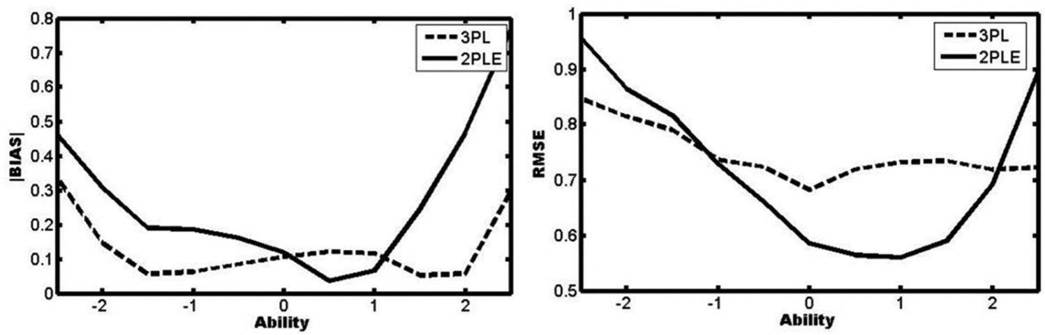
The derivation and implementation of the MLE of θ with the 3PL model can be found in literature (see, e.g., Baker & Kim, 2004; du Toit, 2003). The |BIAS| and RMSE are shown in Figure 5.

Figure 5.

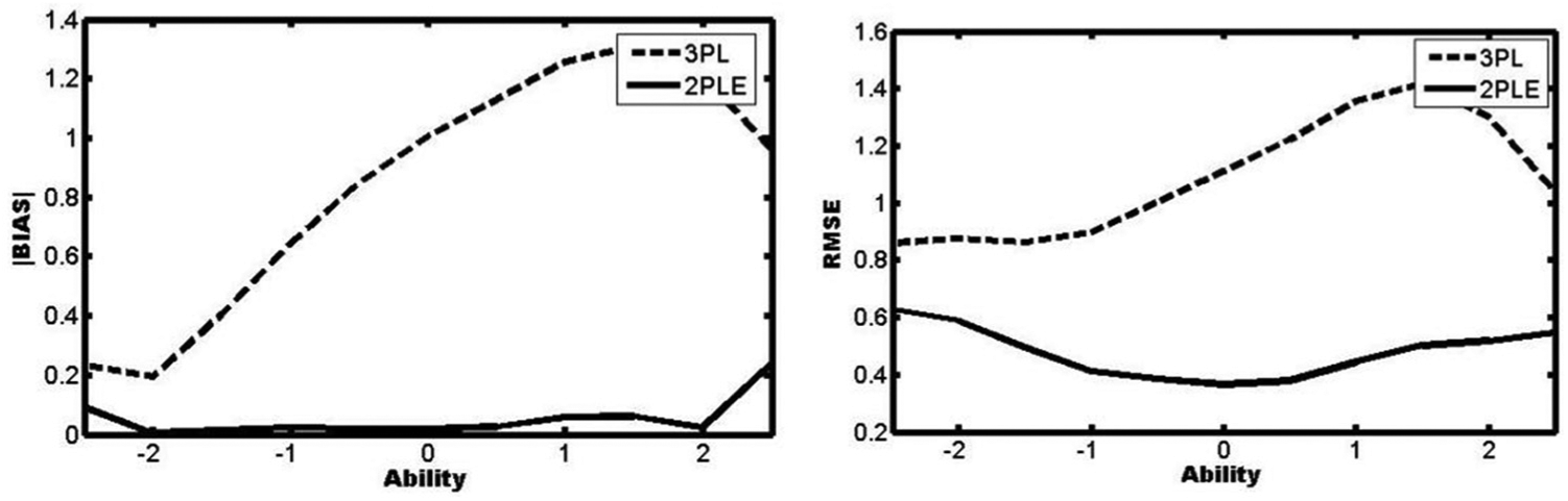
Comparison of the absolute bias (|BIAS|) and RMSE of the ability parameter between the 3PL and 2PLE models in Scenario 1.

In Scenario 1, the 2PLE and 3PL models were both estimated for the data set generated from the 2PLE model. Figure 5 shows that the $| BIAS |$ and RMSE that were computed with the 2PLE model are consistently smaller than those obtained with the 3PL model, illustrating that recovery under the 2PLE model is desirable. By contrast, the 3PL model performs unsatisfactorily when the response data are generated from the 2PLE model.

Scenario 2

In each replication, 20 dichotomous item responses were simulated according to the 2PLE model, and 20 responses were simulated according to the 3PL model. The $| BIAS |$ and RMSE values are shown in Figure 6.

Figure 6.

Comparison of the absolute bias (|BIAS|) and RMSE of the ability parameter between the 3PL model and the 2PLE model in Scenario 2.

In Scenario 2, the 2PLE and 3PL model parameters were estimated with a mixed data set. Figure 6 shows that nearly all the values of $| BIAS |$ and RMSE using the 2PLE model are smaller than those using the 3PL model, illustrating that the 2PLE model performs acceptably well when the model that produces true data is unknown.

Scenario 3

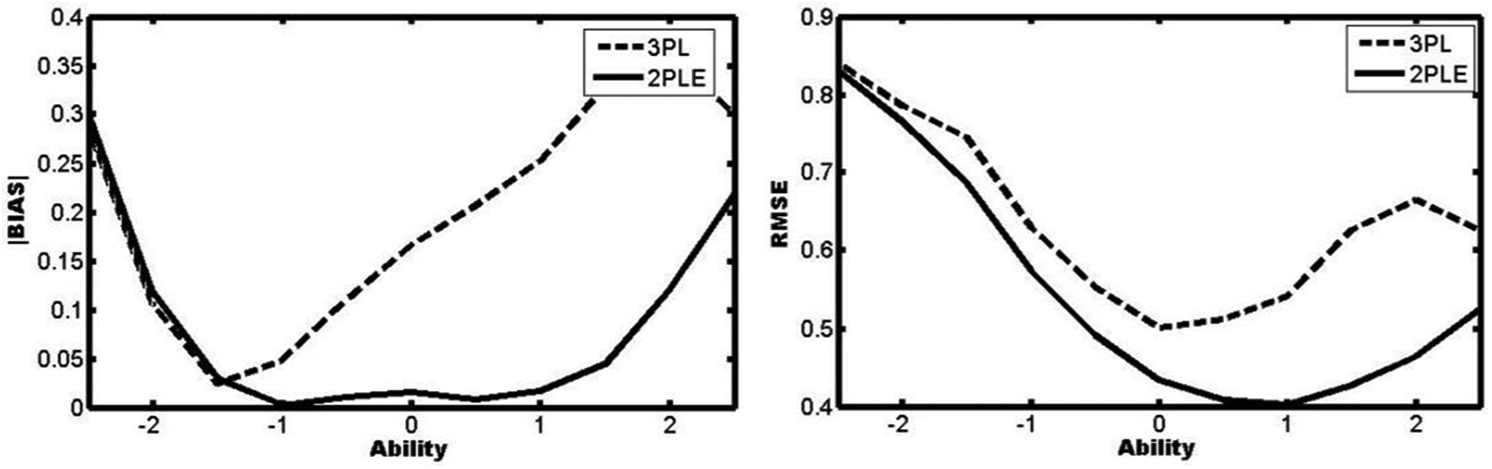
In each replication, 40 dichotomous item responses were simulated according to the 3PL model. The same item responses were used for the 2PLE and 3PLE models for the estimation of ability parameters. The $| BIAS |$ and RMSE values are shown in Figure 7.

Figure 7.

Comparison of the absolute bias (|BIAS|) and RMSE of the ability parameter between the 3PL model and the 2PLE model in Scenario 3.

In Scenario 3, the 2PLE and 3PL model parameters were estimated by using the data generated from the 3PL model. Figure 7 shows that the $| BIAS |$ values using the 3PL model are smaller than those using the 2PLE model. However, the differences in $| BIAS |$ between the 3PL and 2PLE models are close to 0.2 when $θ \leq 1.5$ , and the $| BIAS |$ values of the 3PL and 2PLE models are almost equal near when $θ = 0$ . The RMSE values using the 3PL model are smaller than those using the 2PLE model when $θ < - 1$ and $θ > 2$ but larger than those using the 2PLE model when $- 1 \leq θ \leq 2$ . This results indicate that the 2PLE model performs satisfactorily even when the response data are generated from the 3PL model.

Model Selection

Table 1 provides the AIC and BIC values in Scenarios 1, 2, and 3.

Table 1.

AIC and BIC Values for Scenarios 1 Through 3.

Scenario	Criterion	2PLE	3PL
1	Average of log-likelihood	−48,722	−49,367
	Average of AIC	97,684	98,974
	Average of BIC	98,448	100,120
	Number of replications selected by AIC	500	0
	Number of replications selected by BIC	500	0
2	Average of log-likelihood	−52,207	−52,446
	Average of AIC	104,654	105,131
	Average of BIC	105,421	106,267
	Number of replications selected by AIC	500	0
	Number of replications selected by BIC	500	0
3	Average of log-likelihood	−54,880	−54,768
	Average of AIC	110,000	109,776
	Average of BIC	110,765	110,923
	Number of replications selected by AIC	41	459
	Number of replications selected by BIC	500	0

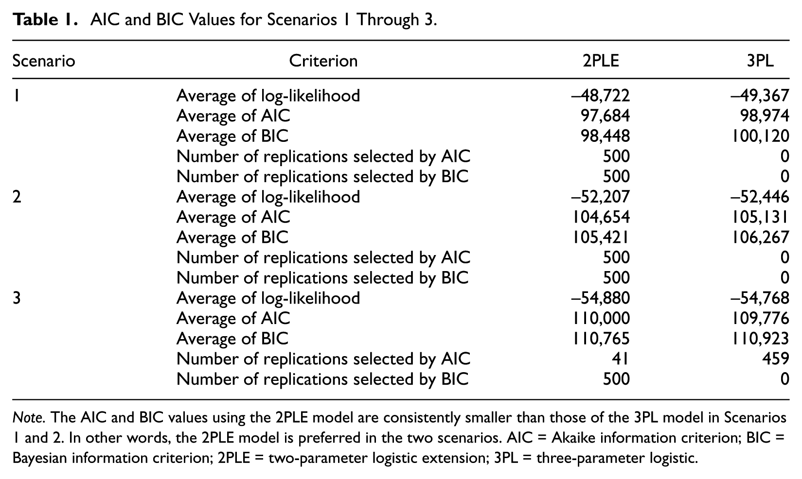
Note. The AIC and BIC values using the 2PLE model are consistently smaller than those of the 3PL model in Scenarios 1 and 2. In other words, the 2PLE model is preferred in the two scenarios. AIC = Akaike information criterion; BIC = Bayesian information criterion; 2PLE = two-parameter logistic extension; 3PL = three-parameter logistic.

In Scenario 3, the AIC from the 2PLE model is larger than that of the 3PL model, but the BIC is smaller for the 2PLE model. This result is consistent with previous findings that AIC tends to select overparameterized models (e.g., Kass & Raftery, 1995), whereas BIC tends to favor parsimonious models. Therefore, in this scenario, the 2PLE model can still be used as a substitute for the 3PL model. Table 1 also presents the number of replications each model is selected by AIC/BIC, and the results are consistent with the findings from the average AIC/BIC. That is, 2PLE is selected by both criteria except in Scenario 3, in which case AIC picks 3PL most of the time.

Real Data Illustration

First, to study the applicability of the 2PLE model, a pilot study was reviewed on a sample of 2000 examinees. The selected test is from a recent state mathematics assessment consisting of 26 items. All multiple-choice items contain four options ( $m_{i} = 4$ ). The results of fitting the models are as shown in Table 2.

Table 2.

Goodness of Fit for the Mathematics Test Data.

Criterion	Model
	1PL-AG	3PL with FLA	1PL-G	2PL	3PL	2PLE
−2LL	61,361	60,724	61,035	60,718	60,746	60,698
AIC	61,467	60,828	61,139	60,822	60,902	60,800
BIC	61,933	61,286	61,597	61,280	61,588	61,258

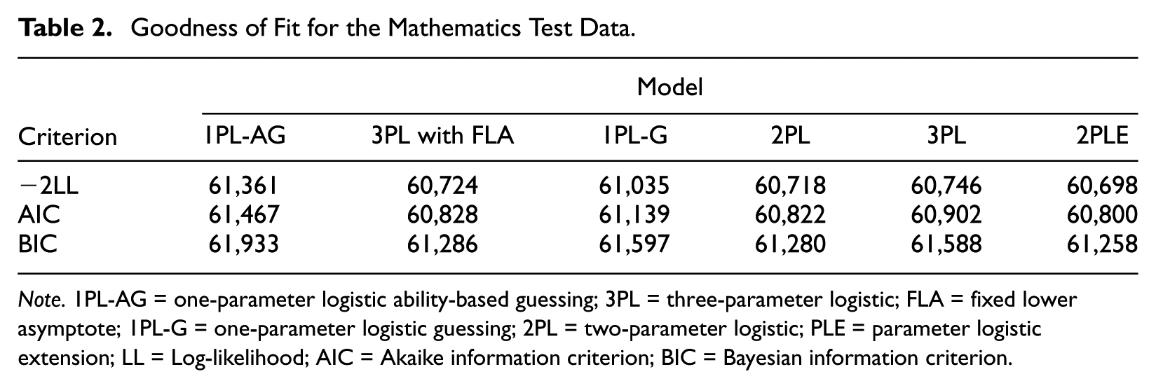
Note. 1PL-AG = one-parameter logistic ability-based guessing; 3PL = three-parameter logistic; FLA = fixed lower asymptote; 1PL-G = one-parameter logistic guessing; 2PL = two-parameter logistic; PLE = parameter logistic extension; LL = Log-likelihood; AIC = Akaike information criterion; BIC = Bayesian information criterion.

Table 2 summarizes the goodness of fit of the six models for the same data set according to the log-likelihood and AIC and BIC values. The goodness of fit of the 2PLE model is clearly better than those of the other models.

Second, the situation in which the number of options of items varied is considered. The Programme for International Student Assessment (PISA) is a triennial international survey that aims to evaluate educational systems worldwide by testing the skills and knowledge of 15-year-old students. More than 70 countries and economies have participated in the assessment. Data from the mathematics exam PISA 2012 in Switzerland based on a sample of 3,397 examinees were used. In this exam, one of the items (PM923Q01) contains five options ( $m_{1} = 5$ ), and each of the other four items contains four options ( $m_{i} = 4$ for $i = 2, . . ., 5$ ).

Table 3 summarizes the goodness of fit of the six models for the data based on the log-likelihood, AIC and BIC values. The AIC and BIC values of the 2PLE model are again the smallest among all models.

Table 3.

Goodness of Fit for the PISA Data.

	Model
Criterion	1PL-AG	3PL with FLA	1PL-G	2PL	3PL	2PLE
−2LL	17,796	17,736	17,773	17,740	17,730	17,729
AIC	17,822	17,772	17,797	17,764	17,754	17,753
BIC	17,916	17,916	17,893	17,860	17,910	17,849

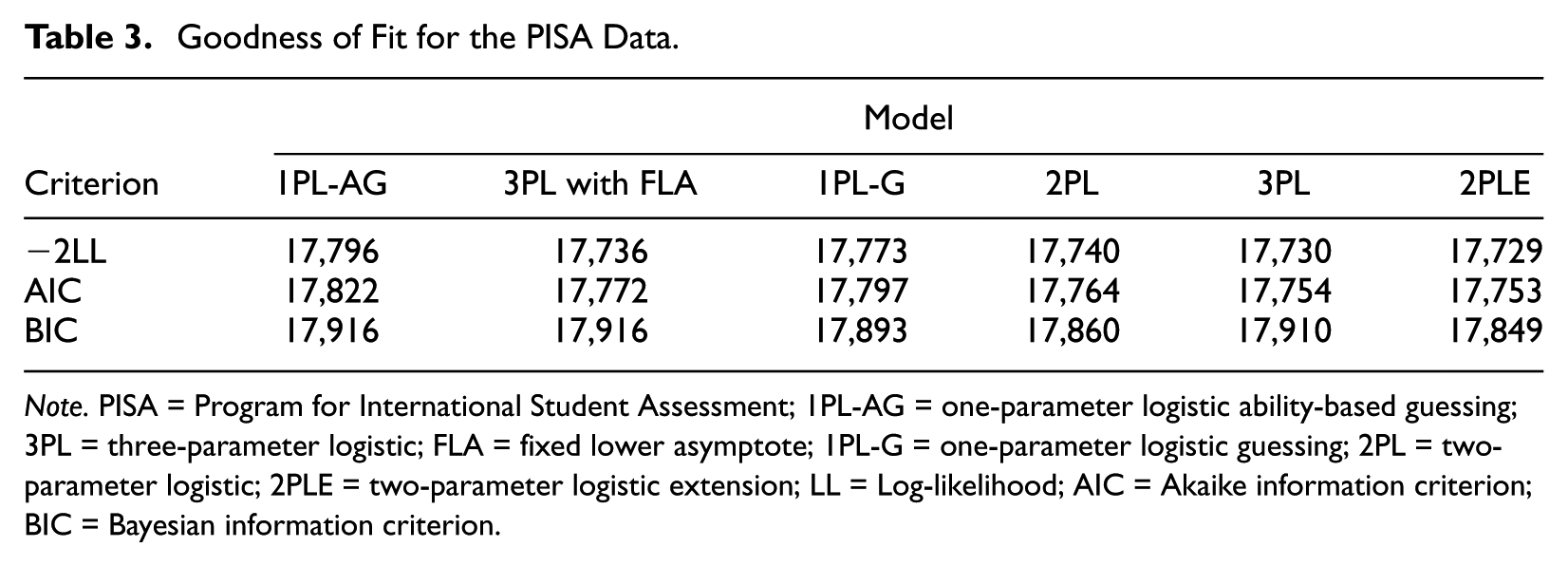
Note. PISA = Program for International Student Assessment; 1PL-AG = one-parameter logistic ability-based guessing; 3PL = three-parameter logistic; FLA = fixed lower asymptote; 1PL-G = one-parameter logistic guessing; 2PL = two-parameter logistic; 2PLE = two-parameter logistic extension; LL = Log-likelihood; AIC = Akaike information criterion; BIC = Bayesian information criterion.

The 1PL-AG, 3PL, 3PL with FLA, and 2PLE models have the same basic structure (Equation 2) but different guessing functions. In these models, the guessing functions of the 1PL-AG and 2PLE models are related to ability. The AIC and BIC values of the former are larger than those of the latter.

Discussion and Conclusion

San Martín et al. (2006) used a two-process theory in cognitive psychology to provide a theoretical foundation for the construction of ability-based guessing model. Extensive research has shown that the probability of a correct guess does not only depend on the item but also on the ability of an individual (Han, 2012; San Martín et al., 2006; van der Maas et al., 2011). Enlightened by the ideas of the above works, the authors proposed the 2PLE model as an alternative to the 3PL model. The key component of the 2PLE model is the IG function. The IG function depends on item characteristics and ability levels. Compared with the 3PL model, the 2PLE model contains one fewer parameter per item, and, therefore, it not only reduces the difficulty of parameter estimation, but it also improves the accuracy of parameter estimation. The simulation results confirmed these advantages in terms of satisfactory parameter recovery and overall model goodness of fit.

Compared to the 1PL-AG model, the 2PLE model has two advantages. First, it allows for item-level discrimination parameter (Lee & Bolt, 2018). Second, the 1PL-AG model contains two distinct sets of item parameters for the problem-solving (b_i) and guessing processes (α, γ_i), respectively. As a result, the interpretation of the item “difficulty” parameter is affected by the guessing process because the overall difficulty of an item is defined by both $b_{i}$ and $γ_{i}$ (Lee & Bolt, 2018). The 2PLE model, on the contrary, uses the same set of item parameters (a_i, b_i) for both processes and, therefore, it allows the outcomes of problem-solving and guessing process to be corrected both across persons and items. This dependency is illustrated in Figure 4, which exemplifies that the item difficulty is reflected in both solution and guessing processes.

From cognitive psychology perspective, Tuerlinckx and De Boeck (2005) discussed the linkage between the 2PL model and the diffusion model for two-choice response processes. Following the same line of reasoning, van der Maas et al. (2011) established the connection of general psychometric models and the Q-diffusion model. This connection provides novel interpretations for the parameters in the 2PL model and other models beyond merely interpreting parameters from a curve-fitting perspective. More importantly, this connection provides new research directions. As an extension of the 2PL model, the 2PLE model preserves the main properties of the 2PL model, such as identifiability and linear invariance. As a result, the establishment of a connection between the 2PLE and diffusion process models represents an interesting yet challenging avenue for further research.

Supplemental Material

Online_Supplement-7-24 – Supplemental material for A Two-Parameter Logistic Extension Model: An Efficient Variant of the Three-Parameter Logistic Model

Supplemental material, Online_Supplement-7-24 for A Two-Parameter Logistic Extension Model: An Efficient Variant of the Three-Parameter Logistic Model by Zhemin Zhu, Chun Wang and Jian Tao in Applied Psychological Measurement

Footnotes

Declaration of Conflicting Interests

The author(s) declared no potential conflicts of interest with respect to the research, authorship, and/or publication of this article.

Funding

The author(s) disclosed receipt of the following financial support for the research, authorship, and/or publication of this article: This research was partially supported by the National Natural Science Foundation of China (Grants 11571069, 11501094) and the Fundamental Research Funds for the Central Universities (Grant 2412017FZ028).

Supplemental Material

Supplemental material is available for this article online.

ORCID iD

^†Jian Tao

References

Baker

F. B.

Kim

S.-H.

(2004). Item response theory: Parameter estimation techniques (2nd ed., rev. and expanded). New York, NY: Marcel Dekker.

Birnbaum

(1968). Some latent trait models and their use in inferring an examinee’s ability. In Lord

F. M.

Novick

M. R.

(Eds.), Statistical theories of mental test scores (pp. 397-479). Reading, MA: Addison-Wesley.

du Toit

. (Ed.). (2003). IRT from SSI: BILOG-MG, MULTILOG, PARSCALE, TESTFACT. Lincolnwood, IL: Scientific Software International.

Frary

R. B.

(1988). Formula scoring of multiple-choice tests (correction for guessing). Educational Measurement: Issues and Practice, 7(2), 33-38.

Hambleton

R. K.

Swaminathan

Rogers

H. J.

(1991). Fundamentals of item response theory. Newbury Park, CA: Sage.

Han

K. T.

(2012). Fixing the c parameter in the three-parameter logistic model. Practical Assessment, Research & Evaluation, 17(1). Retrieved from http://pareonline.net/getvn.asp?v=17&n=1

Holland

P. W.

(1990). The Dutch identity: A new tool for the study of item response models. Psychometrika, 55, 5-18.

Kass

R. E.

Raftery

A. E.

(1995). Bayes factors. Journal of the American Statistical Association, 90, 773-795.

Lee

Bolt

D. M.

(2018). An alternative to the 3PL: Using asymmetric item characteristic curves to address guessing effects. Journal of Educational Measurement, 55, 90-111.

10.

Lord

F. M.

Novick

M. R.

(1968). Statistical theories of mental test scores. Reading, MA: Addison-Wesley.

11.

Maris

(2002). Concerning the identification of the 3PL model (Measurement and Research Department Reports 2003-3). Arnhem, The Netherlands: CITO National Institute for Educational Measurement.

12.

Pelton

T. W.

(2002). The accuracy of unidimensional measurement models in the presence of deviations from the underlying assumptions (Unpublished doctoral dissertation), Department of Instructional Psychology and Technology, Brigham Young University, Provo, UT.

13.

Rasch

(1960). Probabilistic models for some intelligence and attainment tests. Copenhagen, Denmark: Danish Institute for Educational Research.

14.

San Martín

del Pino

de Boeck

. (2006). IRT models for ability-based guessing. Applied Psychological Measurement, 30, 183-203.

15.

San Martín

Gonzáles

Tuerlinckx

. (2015). On the unidentifiability of the fixed-effects 3PL model. Psychometrika, 80, 450-467.

16.

Swaminathan

Gifford

J. A.

(1979). Estimation of parameters in the three-parameter latent trait model (Report No. 90). Amherst: Laboratory of Psychometric and Evaluation Research, School of Education, University of Massachusetts.

17.

Tuerlinckx

De Boeck

(2005). Two interpretations of the discrimination parameter. Psychometrika, 70, 629-650.

18.

van der Linden

W. J.

Hambleton

R. K

. (1997). Handbook of modern item response theory. New York, NY: Springer-Verlag.

19.

van der Maas

H. L. J.

Molenaar

Maris

Kievit

R. A.

Borsboom

. (2011). Cognitive psychology meets psychometric theory: On the relation between process models for decision making and latent variable models for individual differences. Psychological Review, 118, 339-356.

20.

von Davier

. (2009). Is there need for the 3PL model? Guess what?Measurement: Interdisciplinary Research and Perspectives, 7, 110-114.

Supplementary Material

Please find the following supplemental material available below.

For Open Access articles published under a Creative Commons License, all supplemental material carries the same license as the article it is associated with.

For non-Open Access articles published, all supplemental material carries a non-exclusive license, and permission requests for re-use of supplemental material or any part of supplemental material shall be sent directly to the copyright owner as specified in the copyright notice associated with the article.

0.00 MB

0.41 MB

A Two-Parameter Logistic Extension Model: An Efficient Variant of the Three-Parameter Logistic Model

Abstract

Keywords

Introduction and Motivation

Alternative Models With Guessing

Models With Guessing

Motivation of the New Model

The 2PLE Model

Formulation of the Guessing Function, p ( g ) ≡ λ ( θ , δ )

Formulation of the Model

Identifiability of the 2PLE Model

Interpretation of the Model Parameters

Rationality of the 2PLE Model

Simulation and Comparison

Model Comparison

Scenario 1

Scenario 2

Scenario 3

Model Selection

Real Data Illustration

Discussion and Conclusion

Supplemental Material

Online_Supplement-7-24 – Supplemental material for A Two-Parameter Logistic Extension Model: An Efficient Variant of the Three-Parameter Logistic Model

Footnotes

Declaration of Conflicting Interests

Funding

Supplemental Material

ORCID iD

References

Supplementary Material

Formulation of the Guessing Function, $p (g) \equiv λ (θ, δ)$