The EM Algorithm and Its Variants in Cognitive Diagnostic Models: Comparing Their Propensity for Boundaries,Extremes,Convergence,and Suboptimal Solutions

Abstract

Choosing suitable estimation methods for cognitive diagnostic models (CDMs) is critical. However, practitioners often face issues like non-convergence, boundary estimates, extreme values, and unstable suboptimal solutions, which affect the accuracy and reliability of parameter estimates. In this study, we compared expectation–maximization (EM), Bayesian modal estimation (BM), their monotonic constraint variants (EMM and BMM), and variational Bayes (VB) methods. A simulation study was conducted, manipulating factors such as sample size (50, 200, 1000), test length (15, 30), item quality (high, low), and attribute distribution (uniform and multivariate normal). The performance was assessed based on the empirical frequency of each issue, the recovery accuracy of the parameters, and the sensitivity to algorithm initialization. The results, analyzed using the generalized deterministic inputs noisy “and” gate model, reveal three main findings. First, an insufficient sample size was identified as a key factor in problems related to parameter estimation. Second, methods that incorporate prior information (BM and VB) exhibited fewer cases of non-convergence and extreme estimates than EM. Third, the sensitivity analysis showed that the stability of solutions was affected by the choice of initial values, emphasizing the need for proper initialization to reduce the risk of becoming trapped in local suboptimal solutions. This systematic comparison demonstrates that no single estimator is universally superior, and the choice depends on practical constraints. Our findings offer evidence-based guidance for selecting context-sensitive methods, thereby improving the validity of CDMs in real-world applications.

Keywords

cognitive diagnostic models MLE-EM parameter estimation boundary values extreme values convergence local maxima

Introduction

Cognitive diagnostic models (CDMs), or diagnostic classification models (DCMs), provide a statistical framework for evaluating examinees’ detailed latent attributes such as knowledge, strategies, skills, and psychological disorders. These models are commonly used in education, psychology, and psychiatry (Paulsen & Valdivia, 2021; Rupp et al., 2010). Accurate parameter estimation is crucial not only for diagnosing students’ strengths and weaknesses to guide personalized interventions but also for supporting statistical applications, such as item-level model comparison (Buse, 1982; de la Torre & Lee, 2013) and the detection of differential item functioning (Hou et al., 2014; Milewski & Baron, 2002).

Marginalized maximum likelihood estimation using the expectation-maximization algorithm (MLE-EM or EM; de la Torre, 2009, 2011) is an important method for estimating the parameters of CDMs. Packages in R, such as CDM (George et al., 2016) and GDINA (Ma & de la Torre, 2020), as well as software like flexMIRT, Latent GOLD, mdltm, and Mplus (Sen & Terzi, 2020; Templin & Hoffman, 2013), implement MLE-EM for estimating parameters of CDMs. Several extensions have been developed to enhance MLE-EM, including monotonic constraint EM (EMM), Bayes modal estimation (BM), monotonic constraint BM (BMM), and variational Bayes inference (VB; Ma & Jiang, 2021; Yamaguchi & Okada, 2020).

Despite its widespread use, MLE-EM is very sensitive to sample characteristics (Paulsen & Valdivia, 2021; Sessoms & Henson, 2018; Wang et al., 2024). In addition to concerns about general accuracy, practitioners often face several undesirable outcomes, including non-convergence (Templin & Bradshaw, 2014), boundary or extreme parameter estimates (DeCarlo, 2011; Mislevy, 1986), and a tendency to converge to local rather than global optima. These issues can significantly undermine the validity and interpretability of CDMs. In the following sections, we discuss each of these issues in turn.

Boundary Estimates

For DCMs, boundary estimates may occur when parameter values approach the limits of the parameter space (e.g., near 0 or 1) (DeCarlo, 2011; Garre & Vermunt, 2006; Maris, 1999; Yamaguchi, 2023). The sample size requirements are always influenced by the number of attributes involved and their distribution across the items. When test items require many attributes, especially all or most, insufficient sample sizes can result in sparse data for certain attribute profiles, pushing estimates toward the boundaries. This problem is particularly severe when a large number of attributes are combined with a complex Q-matrix (Yamaguchi, 2023). When parameters are close to boundary values, the Fisher matrix can become unstable, causing standard errors (SEs) to be inaccurate. Although Bayesian methods with informative priors have been proposed to address this issue (Harwell & Janosky, 1991; Ma & Jiang, 2021; Mislevy, 1986; Swaminathan & Gifford, 1986), most current approaches overlook structural parameters, which represent the proportions of attribute mastery profiles (Liu et al., 2022). Additionally, choosing appropriate priors in practice is challenging, and misspecified priors can introduce significant bias into parameter estimates (DeMars & Satkus, 2024).

Extreme Parameter Values

Extreme parameter estimates—abnormally high or low values—occur when the observed data lack sufficient power to distinguish among specific parameters (e.g., main effects and interaction effects) (Mislevy, 1986). Consequently, estimation algorithms often fail to converge on a unique optimal solution, leading to unreliable estimates. This issue is especially critical for item parameters (e.g., those representing main and interaction effects), as extreme values can reduce model interpretability. Although Bayesian regularization can help by limiting extreme estimates, its success depends heavily on the proper specification of prior distributions.

Convergence to Local Optima

When the log-likelihood function is convex, it has a single peak and will converge to the global optimum regardless of the starting point (Balakrishnan et al., 2017). However, the multimodal nature of log-likelihood functions, which is common in discrete latent variable models, often causes the EM algorithm to converge to local optima (Shireman et al., 2017). This issue worsens as more latent components are added (Brusa et al., 2024). In CDMs, the discrete latent structure and model complexity worsen this non-convexity problem. As a result, MLE-EM may get trapped in local optima, which are influenced by the choice of initial values. This leads to suboptimal solutions and slow convergence (Gupta & Chen, 2010; Kang et al., 2023; Kuroda & Geng, 2023; Schepers, 2015). R packages like GDINA typically use a single starting value for EM iterations. The algorithm is sensitive to initial values. Different starting points can produce varying results, which affects the stability and reliability of parameter estimation.

Non-Convergence

The convergence rate is a crucial indicator for assessing the performance of an estimation method (Gupta & Chen, 2010; Philipps et al., 2021; Schepers, 2015). When an iterative parameter estimation method fails to converge during later stages, it produces no usable estimates—not even approximate ones, after extensive computation. The MLE-EM iterates between the E-step and M-step until it meets a convergence criterion or reaches the maximum number of iterations (George et al., 2016; Ma & de la Torre, 2020). Convergence failure is a common problem in parameter estimation for CDMs, especially when the sample size is small. Templin and Bradshaw (2014) reported that only 66% to 89% of replications converged in their simulations. Additionally, an overly lenient (i.e., not sufficiently stringent) tolerance can cause the algorithm to halt prematurely, which can result in an inaccurate solution (Karlis & Xekalaki, 2003; Philipps et al., 2021).

Although new methods (e.g., BMM, VB) have been developed to improve parameter estimation in CDMs, existing research focuses primarily on estimation accuracy. This focus leaves important practical issues inadequately addressed, such as algorithmic convergence, boundary and extreme solutions, and sensitivity to initial values. Therefore, this study systematically compares the estimation accuracy and the prevalence of estimation anomalies (non-convergence, boundary values, extreme estimates, and suboptimal solutions) across estimation methods under varying data conditions. This targeted comparison provides a more comprehensive and practical evaluation, filling a gap not sufficiently explored in prior research. We believe this comparison provides valuable practical insights, providing evidence-based guidance to practitioners in choosing suitable estimation methods for CDMs.

The remainder of this paper is organized as follows. First, we introduce the process of estimating the parameters of CDMs using MLE-EM and its variant methods (EMM, BM, BMM, and VB). Next, we present a simulation study to compare the performance of these methods. Finally, in the “Summary and Discussion” section, we summarize the findings and discuss implications for future research.

Method

An Overview of CDMs

Examinees’ test performances reflect their latent general abilities. Cognitive diagnostic assessment decomposes this abstract ability into specific attributes or skills, where mastery of an attribute indicates possession of the corresponding ability (Paulsen & Valdivia, 2021). CDMs demonstrate the relationship between these latent attributes and item responses (Sen & Terzi, 2020). Based on the theoretical assumptions, CDMs can be categorized as constrained or general models. Popular constrained models include the deterministic input, noisy “and” gate (Haertel, 1989); deterministic input, noisy “or” gate (Templin & Henson, 2006); noisy input, deterministic “and” gate model (Junker & Sijtsma, 2001); and noisy input, deterministic “or” gate (Junker & Sijtsma, 2001). General models, such as the general diagnostic model (von Davier, 2005), the log-linear cognitive diagnostic model (LCDM; Henson et al., 2009), and the generalized deterministic inputs, noisy “and” gate model (G-DINA; de la Torre, 2011), provide more flexible parameterizations. Due to its flexibility and comprehensive implementation in the R package, we focus on the G-DINA model in the next section.

G-DINA Model

Suppose N examinees take a test with J items and K attributes. The response matrix $X = (x_{n j}) \in {0, 1}^{N \times J}$ indicates whether examinee n answers item j correctly ( $x_{n j} = 1$ ) or incorrectly ( $x_{n j} = 0$ ). The Q-matrix $Q = (q_{j k}) \in {0, 1}^{J \times K}$ specifies the item–attribute relationships, where $q_{j k}$ = 1 indicates that item j requires attribute k, and $q_{j k}$ = 0 otherwise. The reduced attribute mastery pattern for item j is $α_{l j}^{*} = {(α_{l j 1}, \dots, α_{l j K_{j}^{*}})}^{⊤}$ , where $l = 1, \dots, 2^{K_{j}^{*}}$ . $K_{j}^{*} = \sum_{k = 1}^{K} q_{j k}$ denotes the number of attributes required by item j. The item response function for the identity-link G-DINA model is expressed as follows

P_{l j} = δ_{j 0} + \sum_{k = 1}^{K_{j}^{*}} δ_{j k} α_{l j k} + \sum_{k^{'} = k + 1}^{K_{j}^{*}} \sum_{k = 1}^{K_{j}^{*} - 1} δ_{j k k^{'}} α_{l j k} α_{l j k^{'}} + \dots {+ δ}_{j 12 \dots K_{j}^{*}} \prod_{k = 1}^{K_{j}^{*}} α_{l j k} .

(1)

δ_{j 0}

represents the baseline probability of a correct response when none of the required attributes are mastered.

δ_{j k}

represents the main effect of

α_{l j k}

δ_{j k k^{'}}

represents the interaction effect of attributes

α_{l j k}

and

α_{l j k^{'}}

δ_{j 12 \dots K_{j}^{*}}

is the interaction effect of all required attributes.

The saturated model has $L = 2^{K}$ possible mastery patterns. $π_{l}$ is the mixing proportion parameter, representing the population proportion of individuals with the attribute mastery pattern $α_{l}$ . $π = {(π_{1}, \dots, π_{l}, \dots, π_{L})}^{⊤}$ contains these structural parameters, constraint by $\sum_{l = 1}^{L} π_{l} = 1$ and $π_{l} \geq 0$ (Liu et al., 2022). We chose the G-DINA model due to its flexibility and the comprehensive support offered by the GDINA package in R. Unlike reduced models (e.g., the DINA model) that rely on restrictive assumptions, the G-DINA framework includes intercept, main-effect, and interaction parameters. This enables it to accommodate a broader range of cognitive processes, making it an ideal framework for comparing estimation methods. It has been widely used in simulation studies and empirical data analysis (e.g., Ma & Jiang, 2021; Yamaguchi & Templin, 2022; Zhao et al., 2025). The G-DINA model was used in our simulation study. This choice is not intended to reflect typical applied practice, where more reduced models and model selection procedures are generally preferred.

MLE-EM and Variant Methods for Estimating the Parameters of CDMs

MLE-EM for the G-DINA Model

We use the G-DINA model as an example to illustrate parameter estimation using the MLE-EM. The algorithm starts with an initial set of values, denoted as $γ^{(0)}$ . In the expectation step (E-step), it computes the expected complete-data log-likelihood

Q (γ; γ^{(t)}) = E_{y | x, γ^{(t)}} [\log L (γ; y)] .

(2)

Here,

γ = {(δ^{⊤}, π^{⊤})}^{⊤}

y = (\begin{array}{l} y_{1} \\ ⋮ \\ \begin{array}{l} y_{n} \\ ⋮ \\ y_{N} \end{array} \end{array}) = (\begin{array}{l} \begin{array}{l} x_{1} \\ ⋮ \\ x_{n} \end{array} & \begin{array}{l} α_{1} \\ ⋮ \\ α_{n} \end{array} \\ \begin{array}{l} ⋮ \\ x_{N} \end{array} & \begin{array}{l} ⋮ \\ α_{N} \end{array} \end{array})

, and

γ^{(t)}

is the parameter estimates from the t-th iteration. The expectation is taken over the latent attribute profiles, given the observed data and the parameters

γ^{(t)}

Then, the algorithm calculates the expected posterior probabilities as follows

P (α_{l} | x_{n}, γ^{(t)}) = \frac{P (x_{n} | α_{l}, γ^{(t)}) π_{l}}{\sum_{l = 1} P (x_{n} | α_{l}, γ^{(t)}) π_{l}},

(3)

Where

P (x_{n} | α_{l}, γ^{(t)}) = \prod_{j = 1}^{J} P_{l j}^{x_{n j}} {(1 - P_{l j})}^{1 - x_{n j}}

. The expected counts are computed as follows

n_{l} = \sum_{n = 1}^{N} P (α_{l} | x_{n}, γ^{(t)}),

(4)

r_{l j} = \sum_{n}^{N} x_{n j} P (α_{l} | x_{n}, γ^{(t)}) .

(5)

n_{l}

represents the expected number of examinees in class

α_{l}

, while

r_{l j}

is the expected number of examinees in

α_{l}

who answer item j correctly.

In the maximization step (M-step), these expectations are used to update the parameters to $γ^{(t + 1)}$ by maximizing the $Q$ function (Dempster et al., 1977; Ma & de la Torre, 2020). The updated parameters are

P_{l j} = \frac{r_{l j}}{n_{l}},

(6)

π_{l} = \frac{n_{l}}{N} .

(7)

The updated parameters replace $γ^{(t)}$ in the next E-step. This process continues until the changes in parameter estimates fall below a pre-specified convergence threshold or until the maximum number of iterations is reached.

Bayesian Modal Estimation and Monotonic Constraints

Ma and Jiang (2021) proposed the use of informative priors to improve the MLE-EM estimation in CDMs, and introduced BM estimation for small samples. They demonstrated that when a Beta distribution, $Beta (β_{1}, β_{2})$ , is used as the prior for $P (x_{n j} = 1 ∣ α_{l j}^{*})$ , the posterior distribution also follows a Beta distribution, $Beta (r_{j l} + β_{1}, n_{l} - r_{j l} + β_{2})$ . Thus, the BM estimate is

\hat{P} (x_{n j} = 1 ∣ α_{l j}^{*}) = \frac{r_{j l} + (β_{1} - 1)}{n_{l} + (β_{1} + β_{2} - 2)} .

(8)

For items measuring multiple attributes, latent groups mastering more attributes should have equal or higher correct-answer probabilities than those mastering fewer. Violations of the monotonicity (e.g., $P (101) < P (100)$ ) are theoretically implausible and complicate interpretation (Rupp et al., 2010). However, most methods do not enforce such constraints. Rupp et al. (2010) applied a monotonicity constraint to the LCDM using Mplus. Hong et al. (2016) introduced an order-constrained parameter space for the G-DINA model and proposed corresponding estimation algorithms. Ma and Jiang (2021) recommended incorporating monotonic constraints during model calibration. This can be achieved by optimizing within the M-step of the EM algorithm. Specifically, the procedure involves two steps: (1) Define monotonicity constraints for an item that measures $K_{j}^{*}$ attributes

P (α_{l j}^{*}) \leq P (α_{l^{'} j}^{*}) if α_{l j}^{*} \leq α_{l^{'} j}^{*}

(9)

Where

α_{l j}^{*} \leq α_{l^{'} j}^{*}

indicates that the attribute pattern

α_{l j}^{*}

is a subset of

α_{l^{'} j}^{*}

(Ma & Jiang, 2021). (2) Reformulate the M step as a constrained optimization problem: instead of employing closed-form updates (as in equation (6)), sequential quadratic programming (Kraft, 1988) is employed to solve

M a x i m i z a Q (γ) subject to C \cdot P_{j} \geq 0

(10)

Here, $Q (γ)$ is the expected log-likelihood, $P_{j} = {[P (α_{1 j}^{*}), \dots, P (α_{2^{K^{*}} j}^{*})]}^{⊤}$ is the vector of correct-response probabilities. $C$ is a constraint matrix encoding all pairwise monotonicity constraints (Ma & Jiang, 2021).

Variational Bayes Inference Algorithm

Yamaguchi and Okada (2020) developed a VB inference algorithm for parameter estimation in saturated CDMs. In VB, the prior for the correct response probability parameter $P (α_{j h}^{*})$ is a beta distribution with hyperparameters $a_{j h}^{0}$ and $b_{j h}^{0}$ , where $h = 1, \dots, 2^{K_{j}^{*}}$

P [P (α_{j h}^{*}) | a_{j h}^{0}, a_{j h}^{0}] \propto [{P (α_{j h}^{*})}^{a_{j h}^{0} - 1}] {[1 - P (α_{j h}^{*})]}^{b_{j h}^{0} - 1} .

(11)

The prior for $π$ is a Dirichlet distribution with hyperparameters $λ^{0} = {(λ_{1}^{0}, \dots, λ_{l}^{0}, \dots λ_{L}^{0})}^{⊤}$

P (π | λ^{0}) \propto \prod_{l} π_{l}^{λ_{l}^{0} - 1} .

(12)

The prior for the latent class indicator variable is a categorical distribution

P (z_{n} | π) \propto \prod_{l} π_{l}^{z_{n l}},

(13)

Where the latent class indicator

z_{n} = {(z_{n 1}, \dots, z_{n l}, \dots, z_{n L})}^{⊤}

is a binary (0 or 1) vector that

\sum_{l = 1}^{L} z_{n l} = 1

. VB estimation iteratively maximizes the lower bound of marginal likelihood in a similar manner to the EM algorithm.

Simulation Study

Design

We manipulated four factors: (1) Sample size ( $N = 50$ for classroom-level testing and $N = 200, 1000$ for broader educational assessments (Sen & Cohen, 2021)); (2) test length (J = 15 and 30 representing short-form and standard-length diagnostic instruments, respectively); (3) item quality (IQ), with low-quality items $P (0) = 0.2, P (1) = 0.8$ and high-quality items $P (0) = 0.1, P (1) = 0.9$ ; and (4) attribute distribution (uniform and multivariate normal cases). K (the number of attributes) was fixed at 5. For the multivariate normal condition, data were generated from an $M V N (0_{K}, Σ)$ distribution (Chiu et al., 2009), where Σ has 1s on the diagonal and off-diagonal entries drawn from $U (0, 0.8)$ . These factors were selected to reflect realistic contexts in which CDMs are administered. For each condition, 200 replications were used, and the G-DINA model was used to analyze all data.

This simulation study systematically compares the performance of various CDM parameter estimation methods—EM, EMM, BM, BMM, and VB—in addressing common issues such as non-convergence, boundary estimates, extreme values, and local optima. Figure S2 (Appendix) presents the Q-matrices used in the simulation study.

Data Generation

We employed G-DINA as the model for data generation in the simulation study. Data were generated using the simGDINA function from the GDINA package in R. For the high item quality conditions, the true guessing and slipping parameters were set to 0.1. For the low item quality conditions, both parameters were set to 0.2. Under the multivariate normal assumption, the latent abilities of respondents, denoted as $ϑ_{n} = {(ϑ_{n 1}, \dots, ϑ_{n k}, \dots, ϑ_{n K})}^{⊤}$ , were generated from a multivariate normal distribution, $M V N (0_{K}, Σ)$ . The participants’ attribute mastery patterns were determined by comparing $ϑ_{n k}$ with predefined cutoffs. Specifically, for each attribute k, $α_{n k} = 1$ (indicating mastery of that attribute) if $ϑ_{n k} \geq Φ^{- 1} (\frac{k}{K + 1})$ .

The dichotomous response data were generated by first creating a matrix of correct response probabilities, denoted as ${P_{n} = (P_{n 1}, \dots, P_{n j}, \dots, P_{n J})}^{⊤}$ , based on the above procedures. Each entry represented the probability of a correct response for a given examinee-item pair. A random value was drawn from $U (0, 1)$ , and the response was coded as 1 (correct) if the random value was less than the corresponding probability $P_{n j}$ , or 0 (incorrect) otherwise. This procedure yielded the dichotomized response vector $x_{n} = {(x_{n 1}, \dots, x_{n j}, \dots, x_{n J})}^{⊤}$ .

To generate the initial structural parameters $π_{l}^{(0)}$ , we sampled 20,000 observations from $M V N (0_{K}, Σ)$ . These continuous vectors were dichotomized at a zero threshold to simulate attributes mastery patterns for 20,000 samples. The initial structural parameter $π_{l}^{(0)}$ was set to the observed proportion of each unique pattern $α_{l}$ in this large sample. For the initial item parameters $δ^{(0)}$ , the guessing and slipping parameters for each item were independently sampled from $U (0.01, 0.5)$ . This range captures a wide spectrum of realistic item quality, from highly informative (low guessing/slipping) to nearly uninformative—while avoiding numerical instabilities near zero by setting a lower bound of 0.01. The corresponding main and interaction effect parameters in $δ^{(0)}$ were then deterministically calculated from these values using the G-DINA model formula: $\frac{P (1) - P (0)}{2^{K_{j}^{*}} - 1}$ .

Methods for Comparison

The methods compared in the simulation study included the original EM method (de la Torre, 2011), EMM (Ma & Jiang, 2021), BM (Ma & Jiang, 2021), BMM (Ma & Jiang, 2021), and VB (Yamaguchi & Okada, 2020).

We implemented the EM, EMM, BM, and BMM based on the original code provided by Ma and Jiang (2021). For the EM algorithm, initial values were generated using the procedures described above. Convergence was assessed using a tolerance of 10^-8 on the absolute difference in ${\hat{P}}_{l j}$ between consecutive iterations. A maximum of 70,000 iterations was allowed. EMM used the same convergence criteria but incorporated a monotonicity constraint matrix. For BM, following previous study (Ma & Jiang, 2021), the prior distributions were set as follows: $B e t a (1.5, 2.5)$ for $P (0)$ , $B e t a (2.5, 1.5)$ for $P (1)$ , and $B e t a (2, 2)$ for $P (α_{l} \notin {0, 1})$ . The convergence criteria were aligned with those used in EM. The hyperparameters of the beta distributions are detailed in the Appendix. The VB method was adapted from the satu_dcm( ) function in the R package variationalDCM (Yamaguchi & Okada, 2020), using the same convergence criteria as EM. To ensure a fair comparison, the same initial values—including the initial correct-response probabilities and structural parameters—were used across all methods in each replication. The code used in this study is available at: https://osf.io/mwn8b/overview?view_only=d253836aed614807b5c16c6a628a57db

Criteria

We Evaluated the Following Rates of Problematic Estimates

a. The rate of boundary estimates, defined as parameter values less than 10^-5 or greater than 1–10^-5.

b. The rate of non-convergence, defined as replications where the algorithm failed to converge.

c. The rate of extreme parameter estimates, defined as item parameters less than −1 or greater than 1.

The Accuracy of Parameter Estimates Was Evaluated Using Two Metrics

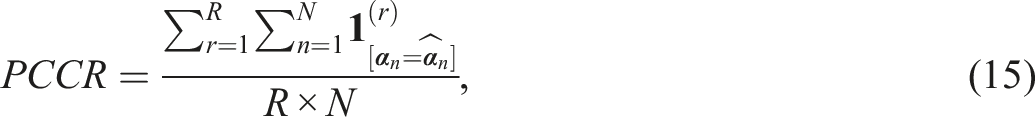
a. The accuracy of correct response parameters (the probabilities of correct answer) was assessed by calculating the mean bias

B i a s (\hat{θ}) = \sum_{r = 1}^{R} \frac{{\hat{θ}}_{r} - θ_{r}}{R},

(14)

Where R is the number of replications, and

{\hat{θ}}_{r}

and

θ_{r}

present the estimated and true correct-response probabilities in replication r, respectively.

b. The recovery of the attribute profiles was measured by the pattern correct classification rate (PCCR)

P C C R = \frac{\sum_{r = 1}^{R} \sum_{n = 1}^{N} 1_{[α_{n} = {\hat{α}}_{n}]}^{(r)}}{R \times N},

(15)

Where

1_{[α_{n} = {\hat{α}}_{n}]}^{(r)}

is an indicator function that equals 1 if the estimated mastery pattern matches the true pattern for examinee n in replication r, and 0 otherwise.

To ensure fair comparisons, criteria (14) and (15) were averaged only over replications in which all compared algorithms converged. This approach ensures that comparisons are based on identical replication sets, thereby avoiding confounding due to convergence proportions. To examine sensitivity to initialization, we performed a separate simulation using a multiple-initialization framework. In this setup, each method was fitted 200 times per replication, with a different set of starting values used for each fitting. This design enables us to isolate and quantify the variability in parameter estimates caused by the choice of initial values.

Sensitivity to Initialization: Unstable Parameter Estimates

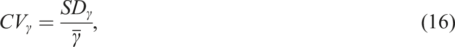
Because directly verifying convergence to a global maximum is challenging, we use the stability of parameter estimates across different initializations as a substitute. The basic idea is that if a unique global maximum exists, estimates should be similar regardless of starting points. On the other hand, large differences in estimates from different initializations suggest convergence to different local optima. Therefore, we compared the coefficient of variation (CV) across initializations to empirically evaluate each method’s sensitivity to initialization.

We quantified the stability of each parameter estimate using its CV, calculated from 200 different sets of initial values in each replication. The CV for parameter $γ$ is defined as

{C V}_{γ} = \frac{{S D}_{γ}}{\bar{γ}},

(16)

Where

{S D}_{γ}

and

\bar{γ}

denote the standard deviation and mean, respectively, of the estimates for parameter

γ

across multiple initializations. Parameters with

{C V}_{γ} > 0.3

were classified as exhibiting substantial instability across initializations.

Results

Non-Convergence Replications Across all Methods

Table 1 presents the number of non-convergent replications across simulation conditions. The BM, BMM, and VB methods achieved 100% convergence under all conditions, whereas convergence issues were exclusive to the EM and EMM. Convergence rates for EM and EMM improved with larger sample sizes, lower item quality, and shorter test lengths. Both methods also converged more frequently under a uniform attribute distribution than under a multivariate normal distribution. The computational time required for each method to converge is provided in Table S1 in the Appendix.

Table 1.

The Non-Convergence Replications of All Methods

J	IQ	N	Att.dist = mvnorm		Att.dist = uniform
J	IQ	N	EM	EMM	EM	EMM
15	High	50	6	3	1	0
15	High	200	0	1	0	0
15	High	1000	0	0	0	0
15	Low	50	0	0	0	0
15	Low	200	0	0	0	0
15	Low	1000	0	0	0	0
30	High	50	69	51	1	1
30	High	200	28	7	0	0
30	High	1000	1	1	0	0
30	Low	50	39	6	1	1
30	Low	200	5	0	0	0
30	Low	1000	0	0	0	0

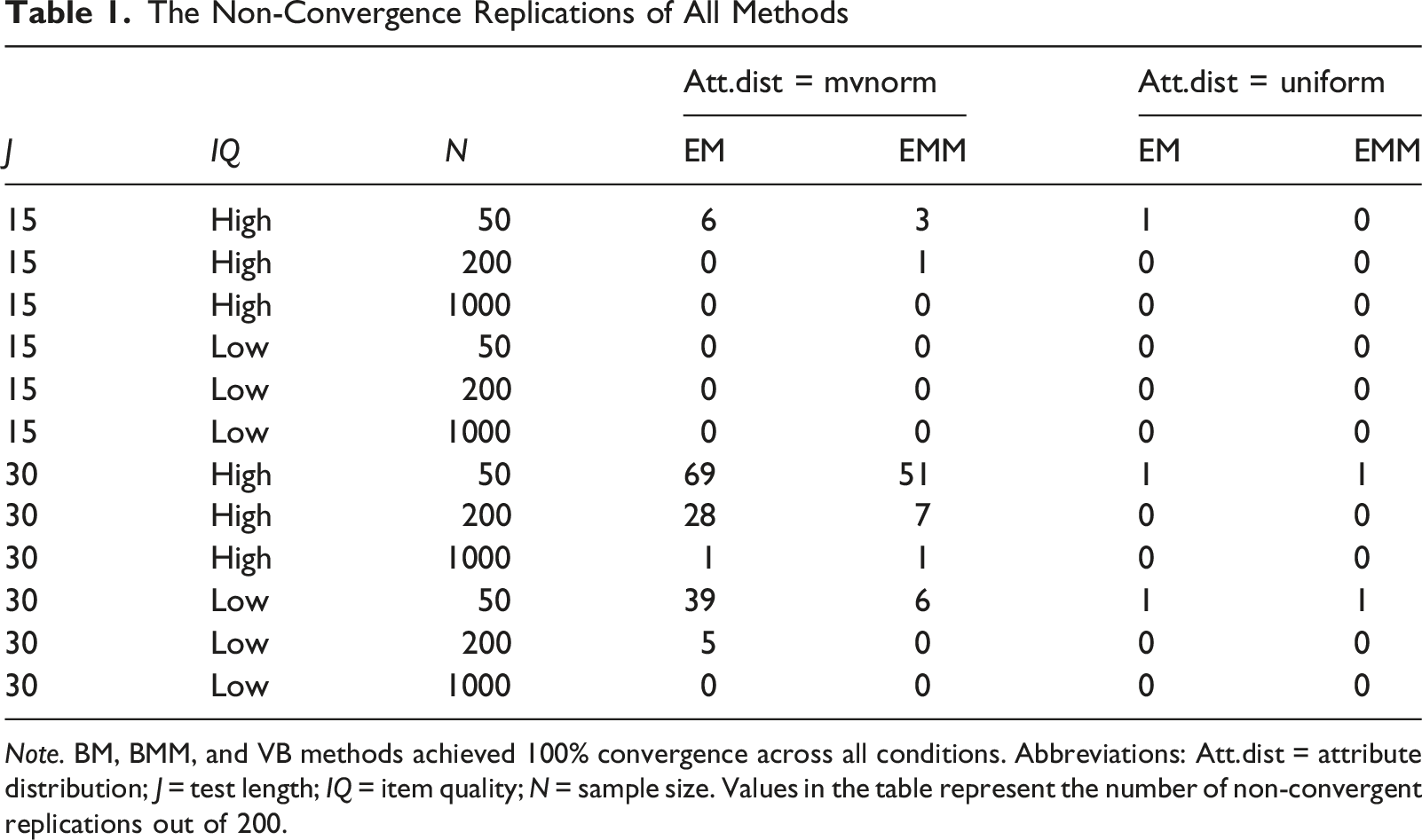
Note. BM, BMM, and VB methods achieved 100% convergence across all conditions. Abbreviations: Att.dist = attribute distribution; J = test length; IQ = item quality; N = sample size. Values in the table represent the number of non-convergent replications out of 200.

We further examined these non-converged cases and observed two patterns. (1) Structural collapse due to empty latent classes. The algorithm terminated with the warning “Nj contains 0.” When there are many latent classes relative to the sample size, some classes receive almost no observations. These cases reflect numerical degeneracy caused by sparse data. (2) The algorithm reaches the maximum number of iterations without meeting the convergence criterion. Examination of the log-likelihood trajectories shows that after an initial phase of rapid improvement, the log-likelihood stabilizes and stays nearly constant over many iterations. However, the maximum parameter change (maxchg) continues to oscillate and does not drop below the convergence tolerance (see Supplemental Figure S3). We tentatively attribute this to flat or weakly identified regions in the later stages of iteration, where local oscillations occur in the parameter space without meaningful improvement in the objective function.

Proportion of Problematic Parameter Estimates

Figures 1 and 2 show the rate of boundary problems for correct response probabilities and structural parameters. Boundary values for response probabilities occurred more often in EM and EMM. This problem was reduced with larger samples and longer tests, and was more frequent under multivariate normal attribute distributions than under uniform distributions. The rate of boundary solutions for structural parameters was much higher than for response probabilities. Except for VB, all estimation methods showed a high rate of boundary solutions in structural parameter estimates. This issue was also reduced by increasing the sample size and test length.

Figure 1.

The rate of boundary problem for correct response probabilities

Figure 2.

The rate of boundary problem for structural parameters. Note. Abbreviations: Att. dist = attribute distribution; J = test length; IQ = item quality (1: high, 2: low); N = sample size. Values in the figure represent the rates of boundary problems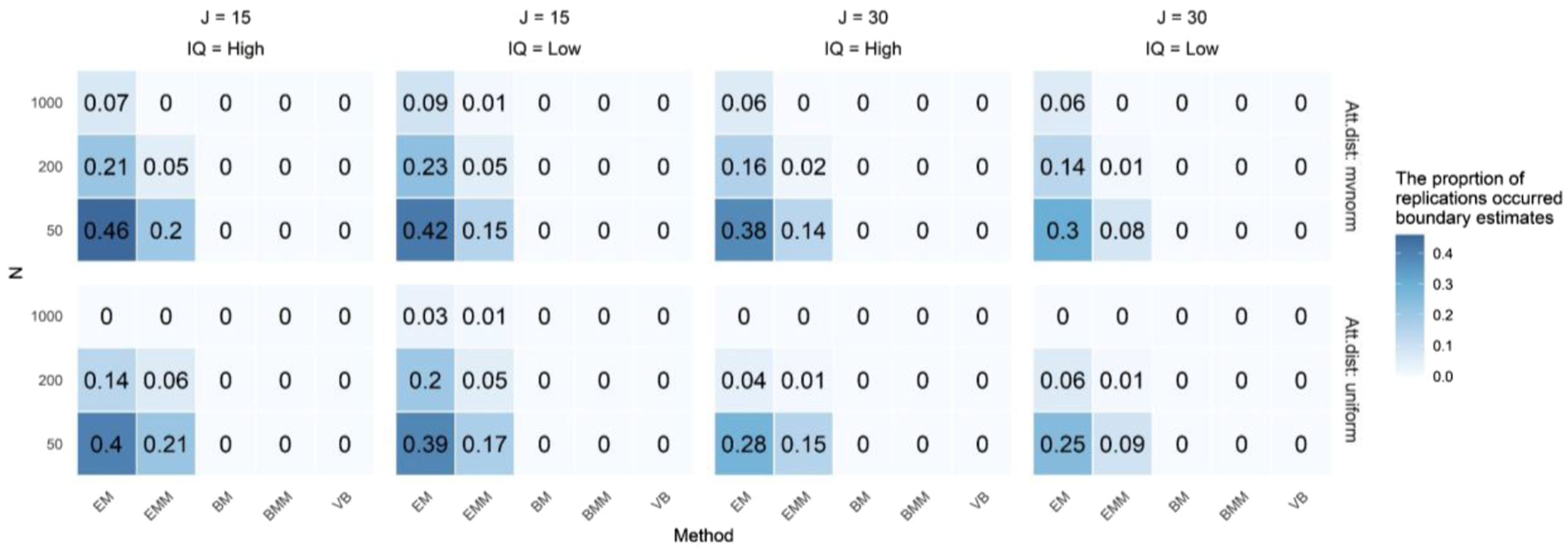

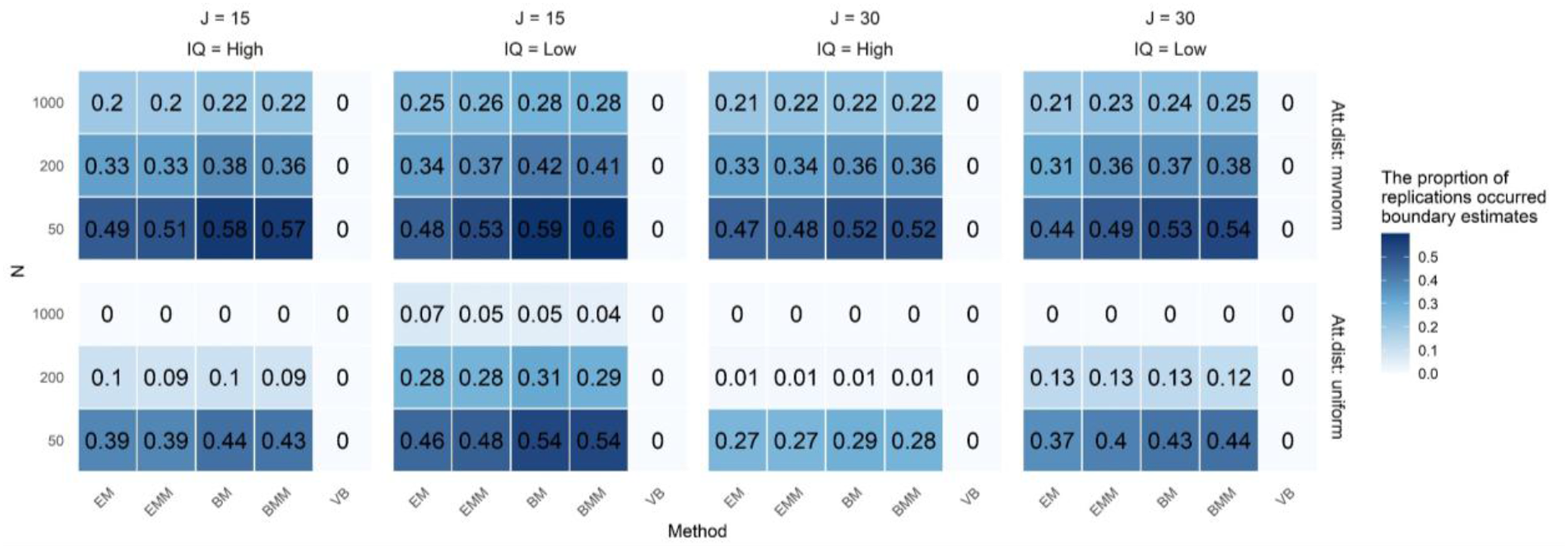
VB showed no boundary estimates for the structural parameters, and this is largely because it uses prior information. While the BM and BMM apply priors solely for the correct response probabilities, VB employs priors for both response probabilities and the structural parameters. This helps regularize estimates and prevents boundary solutions. Further analysis showed that, under the multivariate normal distribution, some attribute mastery patterns appeared infrequently or were missing in the generated data due to sampling error. This scarcity of response data for these rare patterns probably led structural parameter estimates to converge near zero. In real-world applications, such boundary estimates should trigger an examination of the sample and consideration of possible attribute hierarchies. Notably, at a sample size of N = 1000, the occurrence rate decreased significantly, indicating that N = 1000 might serve as a practical benchmark for addressing this issue.

Figure 3 shows the rate of extreme item parameters. Overall, the EM algorithm was most susceptible to this issue, producing the highest rates of extreme problems, especially under conditions of lower item quality, smaller sample sizes, and shorter test lengths. A uniform attribute distribution, compared to a multivariate normal distribution, generally resulted in fewer extreme estimates.

Figure 3.

The rate of extreme problem. Note. Abbreviations: Att. dist = attribute distribution; J = test length; IQ = item quality (1: High, 2: Low); N = sample size. Values in the figure represent the rates of extreme problems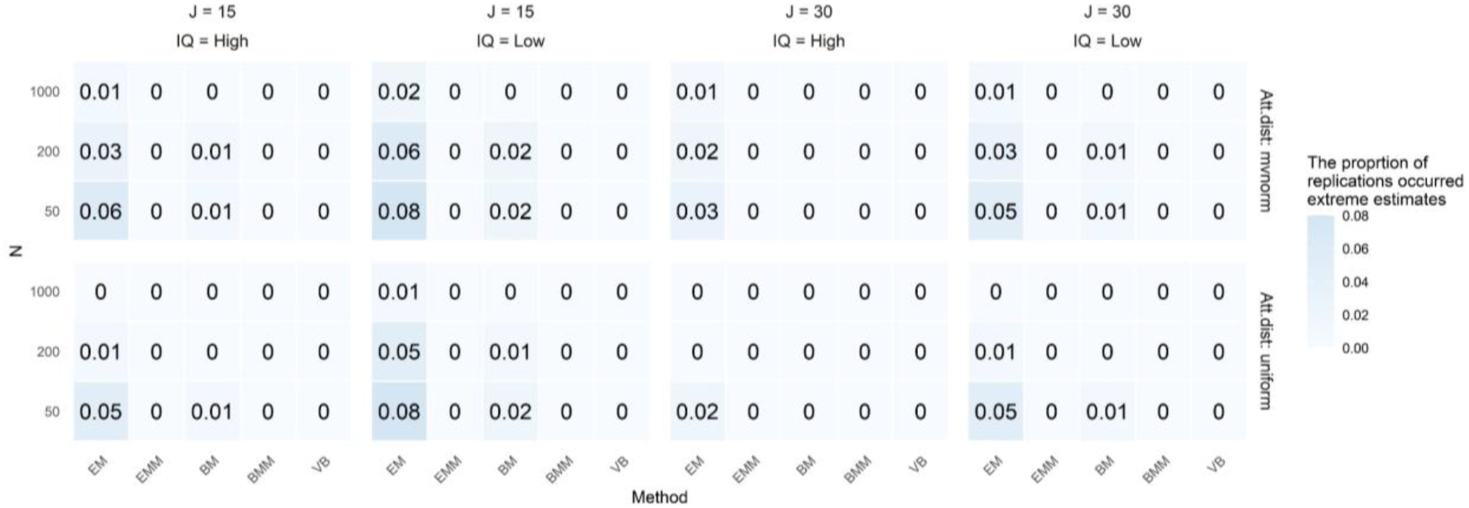

In summary, VB showed better performance in addressing all three issues: non-convergence, boundary estimates, and extreme parameter values. It was the most reliable method in handling non-convergence, which is a clear weakness of the EM method, as well as boundary estimates and extreme parameter values.

These findings support previous research showing that small sample sizes and too many attributes can cause estimation issues (Akbay & de la Torre, 2020; Balakrishnan et al., 2017; Templin & Bradshaw, 2014; Yamaguchi, 2023). VB’s strength comes from its use of informative priors for both item and structural parameters. Proper prior specification is vital in practice because real-world data may involve large sampling errors or hierarchical attribute structures (Akbay & de la Torre, 2020; Balakrishnan et al., 2017; Templin & Bradshaw, 2014).

It is worth noting that the high rates of non-convergence, boundary estimates, and extreme values observed under the N = 50 conditions can be partly attributed to empirical under-identification. In these conditions, the ratio of sample size to freely estimated parameters in the saturated G-DINA model (K = 5) is very low. As this ratio improves at N = 200 and N = 1000, model identifiability increases, and these estimation anomalies decline substantially across all algorithms.

Accuracy of Parameter Estimates

Figure 4 shows a comparison of estimation accuracy based on PCCR and Bias. Recovery metrics were computed using only converged replications. Overall, performance improved consistently with larger sample sizes, longer tests, and higher item quality. In terms of PCCR, the EM method consistently demonstrated the poorest performance, whereas the EMM method slightly outperformed it. Both EM and EMM exhibited more bias in the correct-response parameters than the BM and BMM methods. BMM and BM presented the best overall performance, achieving higher PCCR values and near-zero bias. In contrast, VB exhibited a notable trade-off: it delivered competitive PCCR values, often similar to BMM and BM, but consistently had the worst Bias. For example, under the challenging mvnorm condition (J = 15, IQ = High, N = 50), VB’s PCCR was only surpassed by BM and BMM, but it exhibited significant bias in estimating response probabilities.

Figure 4.

The parameter recovery of all methods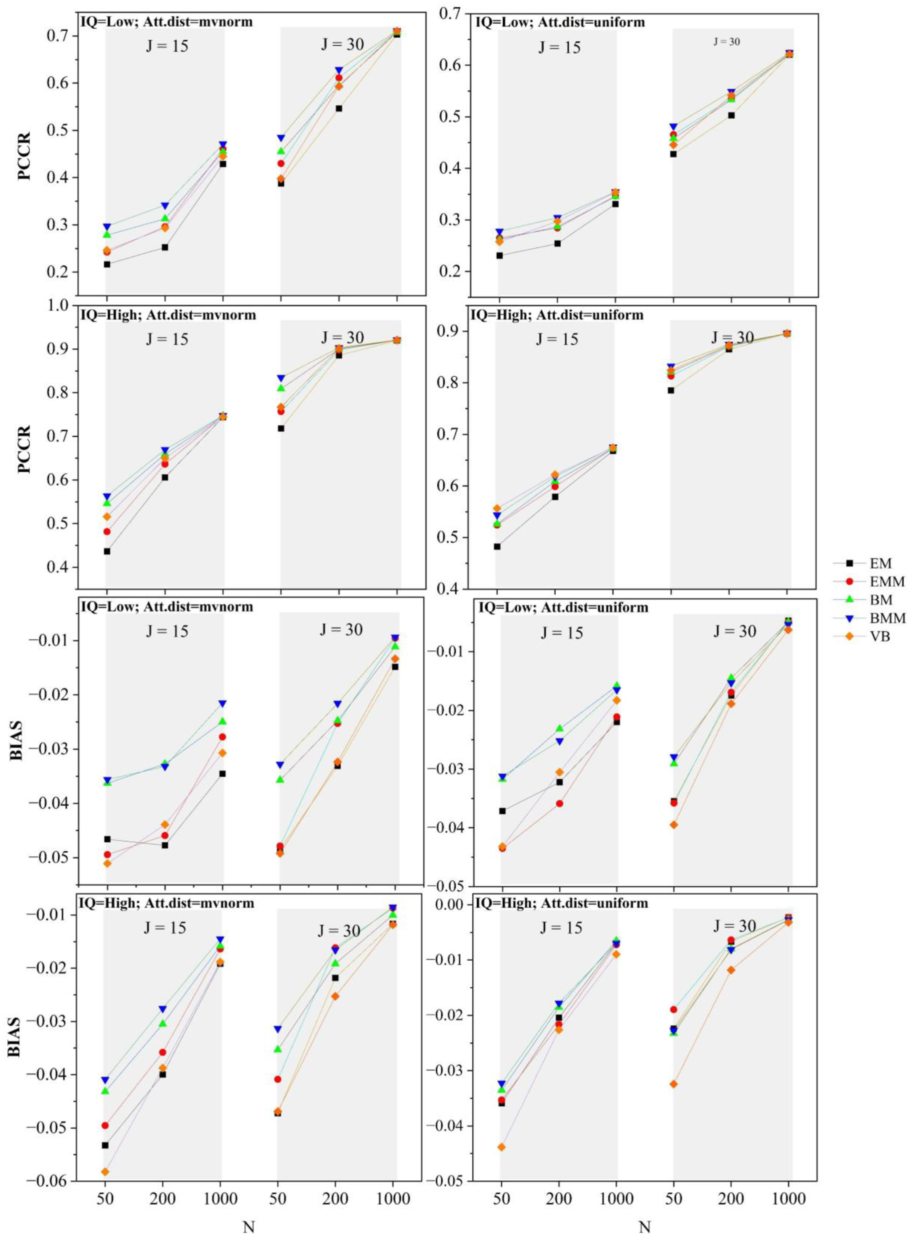

Instances of Monotonicity Constraint Violations

The results in Table 2 show instances where the parameter estimates broke monotonicity rules. For example, for item 21 (Kj = 3, N = 1000, IQ = low, Att. dist = mvnorm), methods that do not enforce monotonicity constraints (EM, BM, and VB) gave estimates that violated a key principle. Specifically, examinees who mastered more attributes were estimated to have a lower probability of answering correctly than those with fewer. Specific violations included

P (101) < P (001)

for EM,

P (011) < P (001)

for BM, and

P (011) < P (001)

for VB. These violations weaken the interpretability of CDMs because they suggest that mastering more attributes might be associated with a lower probability of a correct response.

Table 2.

An Example of Noncompliance with Monotonicity Constraints

	$P (000)$	$P (100)$	$P (010)$	$P (001)$	$P (110)$	$P (101)$	$P (011)$	$P (111)$
EM	0.1364	0.5441	0.4753	0.9999	0.6008	0.7974	0.6050	0.7924
EMM	0.1360	0.5307	0.4622	0.7926	0.5994	0.7926	0.7926	0.7926
BM	0.1507	0.5385	0.4853	0.7467	0.5979	0.7992	0.5259	0.7953
BMM	0.1512	0.5345	0.4762	0.6676	0.5982	0.7946	0.6676	0.7946
VB	0.1455	0.5291	0.4748	0.7491	0.5953	0.7944	0.5327	0. 7925

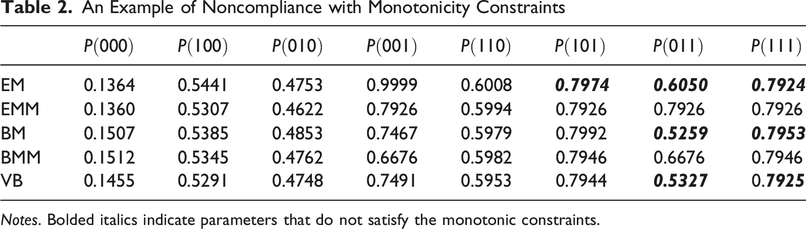
Notes. Bolded italics indicate parameters that do not satisfy the monotonic constraints.

Count of Parameters With High Instability (CV >0.3) Across Initializations

To evaluate the influence of initial values, we examined the coefficient of variation (CV) for each model parameter across 200 different initializations. A parameter was deemed unstable if its CV exceeded 0.3. Figures 5 and 6 display the number of such unstable parameters. The G-DINA model with K = 5 and no hierarchical structure has 32 possible attribute mastery patterns, corresponding to 32 structural parameters. For J = 30 items, the G-DINA model included a total of 172 parameters (32 structural and 140 response probabilities). For J = 15, it had 102 parameters.

Figure 5.

The number of unstable correct response probabilities. Note. Under the G-DINA model, there are 70 correct-response parameters for J = 15 and 140 for J = 30. The numbers in the figures indicate the count of parameters with CV >0.3

Figure 6.

The number of unstable structural parameters. Note. Under the G-DINA model with K = 5, there are 32 structural parameters. The numbers in the figures indicate the count of parameters with CV >0.3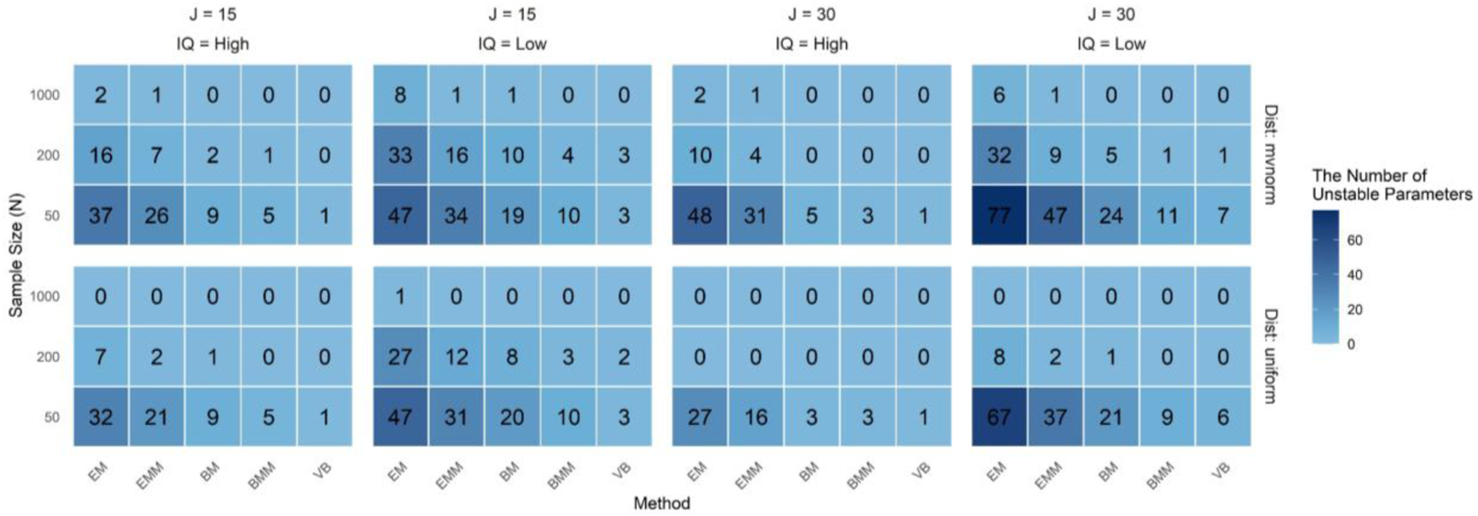

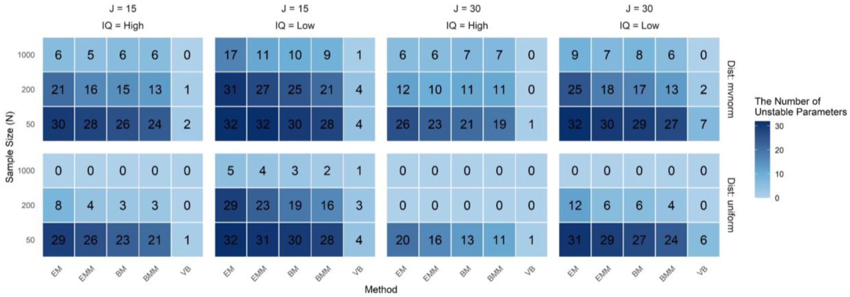
Figure 5 displays the number of unstable response parameters across different conditions. The EM method performed the worst overall. For example, under the conditions of J = 15, N = 50, high item quality, and multivariate normal attribute distribution, 37 out of 70 parameters (about 53%) had CV values higher than 0.3. In comparison, VB demonstrated the best performance, with only 1 unstable parameter under these conditions.

Figure 6 presents the results for structural parameters, showing an even stronger pattern. Under the challenging setting of J = 15, N = 50, high item quality, and multivariate normal distribution, 30 out of 32 structural parameters (94%) were unstable with EM, compared to only 2 with VB. Together with the results in Figure 5, this indicates that 67 out of the total 102 model parameters were unstable under EM initialization, while only 3 were unstable under VB.

These findings strongly indicate that parameter estimation in EM and related methods is highly sensitive to initial values, raising concerns about their reproducibility and reliability in practical applications. EM and EMM exhibited the greatest sensitivity to initialization, followed by BM and BMM, with VB showing better robustness. Moreover, as the sample size increased to N = 1000 and the quality of items improved, parameter stability improved significantly. While increasing sample size improves stability, it is not a complete solution. A robust application also requires careful method selection to mitigate initialization dependence.

In the Supplemental Material, we additionally selected six sets of initial values to illustrate the impact of initialization on the algorithm (see Table S2). The result shows that a different set of initial values may yield a superior value of the objective function. Notably, combined evidence from Figure S3 and Table S2 suggests that the likelihood surface in CDMs is characterized by complex geometry. The likelihood surface is multimodal, with multiple local optima associated with different starting points (Table S2). Within local regions, however, the algorithm may exhibit oscillatory behavior near stationary points where the surface is relatively flat or weakly identified (Figure S3).

Conclusion

Summary and Discussion

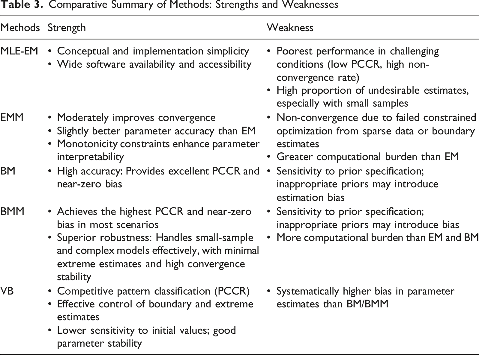
This study examined the occurrence patterns of estimation anomalies, including boundary estimates, extreme values, non-convergence, and suboptimal solutions, across commonly used estimation methods for CDMs under varying data conditions. The goal was to characterize how frequently these issues arise and to offer practical guidance for applied researchers. Table 3 summarizes the advantages and limitations of different parameter estimation methods.

Table 3.

Comparative Summary of Methods: Strengths and Weaknesses

Methods	Strength	Weakness
MLE-EM	• Conceptual and implementation simplicity • Wide software availability and accessibility	• Poorest performance in challenging conditions (low PCCR, high non-convergence rate) • High proportion of undesirable estimates, especially with small samples
EMM	• Moderately improves convergence • Slightly better parameter accuracy than EM • Monotonicity constraints enhance parameter interpretability	• Non-convergence due to failed constrained optimization from sparse data or boundary estimates • Greater computational burden than EM
BM	• High accuracy: Provides excellent PCCR and near-zero bias	•Sensitivity to prior specification; inappropriate priors may introduce estimation bias
BMM	• Achieves the highest PCCR and near-zero bias in most scenarios • Superior robustness: Handles small-sample and complex models effectively, with minimal extreme estimates and high convergence stability	•Sensitivity to prior specification; inappropriate priors may introduce bias • More computational burden than EM and BM
VB	• Competitive pattern classification (PCCR) • Effective control of boundary and extreme estimates • Lower sensitivity to initial values; good parameter stability	• Systematically higher bias in parameter estimates than BM/BMM

Overall, the findings can be understood along three interrelated dimensions: data conditions, model complexity, and algorithmic characteristics. We observed a strong co-occurrence of empirical under-identification, flat likelihood surfaces, and estimation anomalies. First, consistent with prior research, small sample sizes substantially increase the occurrence of estimation anomalies (Oka & Okada, 2022; Sorrel et al., 2023). One plausible explanation is empirical under-identification, particularly under the G-DINA model, where the number of parameters may be large relative to the available sample size, leading to unstable estimation, non-convergence, and boundary solutions.

Second, differences across estimation methods can be interpreted in light of their algorithmic properties. The EM algorithm showed greater sensitivity to initialization and a higher tendency to yield suboptimal solutions, whereas methods incorporating prior information (e.g., BM and VB) demonstrated greater stability. This pattern is consistent with the regularization effect of priors, which constrain the parameter space and reduce the occurrence of extreme or implausible estimates, particularly under sparse data conditions. Similarly, monotonicity constraints (EMM and BMM) may further restrict the parameter space and improve stability in some scenarios. In practice, priors should be specified not only for item parameters but also for structural parameters. Although priors can mitigate extreme and boundary estimates, choosing appropriate priors remains a nontrivial task (DeMars & Satkus, 2024). We recommend the use of weakly informative priors, as overly strong priors may introduce bias. At the same time, boundary values are not always artifacts. For example, when certain attribute profiles are absent in the population, true parameters may legitimately be near zero. Therefore, careful contextual interpretation is required.

It is important to note that these interpretations are based on observed occurrence patterns rather than formal theoretical analysis. Estimation difficulties in CDMs likely arise from multiple sources, including complex likelihood surfaces with potential local optima, sparse data structures, and model specification. A more rigorous analysis of likelihood geometry and identifiability remains an important direction for future work.

Beyond these general mechanisms, two practical determinants of estimation performance are convergence behavior and initialization. Convergence is critical for valid inference. In this study, non-convergence in EM was typically associated with failure to meet the convergence criterion within the maximum number of iterations, while in EMM it was sometimes related to constrained optimization issues (e.g., zero observed counts or boundary solutions). Although relaxing convergence criteria may increase the number of converged replications (Nader et al., 2011), such solutions may reflect premature convergence and should be interpreted cautiously (Philipps et al., 2021). Therefore, relatively strict convergence criteria are recommended in practice, and more systematic validation of convergence warrants further investigation.

Initialization was a key determinant of both solution quality and reproducibility. Using 200 different starting values, we observed substantial variability in outcomes, indicating that estimates can depend on initialization and may be unstable under single-start practices. This has direct implications for reproducibility, which requires consistent results across repeated analyses (National Academies of Sciences, Engineering, and Medicine, 2019). Accordingly, the routine use of multiple random starts is recommended to reduce the risk of converging to suboptimal solutions. Future work should develop more systematic strategies for selecting or screening starting values, as well as more effective global optimization approaches.

Several practical recommendations follow from these findings. First, under limited sample sizes or short tests, methods incorporating prior information (e.g., BM and BMM) are generally preferable due to their greater robustness. Second, maintaining adequate item quality remains essential, as poor item quality negatively affects all estimation methods, particularly EM. In this study, the number of attributes was fixed at $K = 5$ . Although we did not manipulate $K$ , prior studies that varied the number of attributes suggest that larger $K$ would likely further amplify the estimation difficulties observed in this study (Oka & Okada, 2022; Paulsen & Valdivia, 2021; Sessoms & Henson, 2018; Yamaguchi, 2023). Third, no single method is universally optimal; method selection should be guided by data conditions, model complexity, and the primary analytical goal.

In addition, beyond parametric estimation methods, nonparametric methods may serve as useful alternatives in specific contexts. In small-sample settings (e.g., N = 50; Sessoms & Henson, 2018; Sen & Cohen, 2021), nonparametric methods have been shown to perform well for attribute classification (Chiu et al., 2018). Practitioners may therefore consider combining or selecting methods based on their goals—for instance, using nonparametric methods when accurate classification is prioritized (Ma et al., 2023).

Several limitations should be noted. First, this study focused on the occurrence and prevalence of estimation anomalies rather than a formal analytical characterization of their underlying causes. Although we discussed potential explanations, such as empirical under-identification and regularization effects, these interpretations are based on simulation evidence and should not be viewed as definitive causal conclusions.

Second, the use of the G-DINA model should be interpreted as a stress-test scenario. While it enables evaluation of estimation methods under challenging conditions, it may overstate the level of difficulty relative to typical applications. In practice, especially under conditions such as small sample sizes and a moderate number of attributes, more reduced models and formal model selection procedures should be considered.

Future research may extend this work by (1) developing estimation methods that explicitly address sparse data conditions, (2) improving global optimization and initialization strategies, (3) examining a wider range of CDMs and model complexities, and (4) conducting more rigorous theoretical analyses to better understand the structural mechanisms underlying estimation anomalies.

Supplemental Material

Supplemental material—The EM Algorithm and Its Variants in Cognitive Diagnostic Models: Comparing Their Propensity for Boundaries, Extremes, Convergence, and Suboptimal Solutions

Supplemental material for The EM Algorithm and Its Variants in Cognitive Diagnostic Models: Comparing Their Propensity for Boundaries, Extremes, Convergence, and Suboptimal Solutions by Yue Zhao, Tao Xin, Yanlou Liu, and Yiming Wang in Applied Psychological Measurement

Footnotes

ORCID iDs

Yue Zhao

Tao Xin

Yanlou Liu

Yiming Wang

Funding

The authors disclosed receipt of the following financial support for the research, authorship, and/or publication of this article: This research was supported by the National Natural Science Foundation of China (31900794), the Natural Science Foundation of Shandong Province in China (ZR2019BC084), and the National Key R&D Program of China (2021YFC3340801).

Declaration of Conflicting Interests

The authors declared no potential conflicts of interest with respect to the research, authorship, and publication of this article.

Data Availability Statement

The datasets generated during and analyzed during the current study are available in the Open Science Framework (OSF) repository, .

Supplemental Material

Supplemental material for this article is available online.

References

Akbay

de la Torre

(2020). Estimation approaches in cognitive diagnosis modeling when attributes are hierarchically structured. Psicothema, 32(1), 122–129. https://doi.org/10.7334/psicothema2019.182

Balakrishnan

Wainwright

M. J.

(2017). Statistical guarantees for the EM algorithm: From population to sample-based analysis. The Annals of Statistics, 45(1), 77–120. https://doi.org/10.1214/16-AOS1435

Brusa

Pennoni

Bartolucci

(2024). Maximum likelihood estimation for discrete latent variable models via evolutionary algorithms. Statistics and Computing, 34(2), 62. https://doi.org/10.1007/s11222-023-10358-5

Buse

(1982). The likelihood ratio, wald, and lagrange multiplier tests: An expository note. The American Statistician, 36(3), 153–157. https://doi.org/10.1080/00031305.1982.10482817

Chiu

C.-Y.

Douglas

J. A.

(2009). Cluster analysis for cognitive diagnosis: Theory and applications. Psychometrika, 74(4), 633–665. https://doi.org/10.1007/s11336-009-9125-0

Chiu

C.-Y.

Sun

Bian

(2018). Cognitive diagnosis for small educational programs: The general nonparametric classification method. Psychometrika, 83(2), 355–375. https://doi.org/10.1007/s11336-017-9595-4

DeCarlo

L. T.

(2011). On the analysis of fraction subtraction data: The DINA model, classification, latent class sizes, and the Q-matrix. Applied Psychological Measurement, 35(1), 8–26. https://doi.org/10.1177/0146621610377081

de la Torre

(2009). DINA model and parameter estimation: A didactic. Journal of Educational and Behavioral Statistics, 34(1), 115–130. https://doi.org/10.3102/1076998607309474

de la Torre

(2011). The generalized DINA model framework. Psychometrika, 76(2), 179–199. https://doi.org/10.1007/s11336-011-9207-7

10.

de la Torre

Lee

Y.-S.

(2013). Evaluating the wald test for item-level comparison of saturated and reduced models in cognitive diagnosis. Journal of Educational Measurement, 50(4), 355–373. https://doi.org/10.1111/jedm.12022

11.

DeMars

C. E.

Satkus

(2024). Item parameter recovery: Sensitivity to prior distribution. Educational and Psychological Measurement, 84(4), 691–715. https://doi.org/10.1177/00131644231203688

12.

Dempster

A. P.

Laird

N. M.

Rubin

D. B.

(1977). Maximum likelihood from incomplete data via the EM algorithm. Journal of the Royal Statistical Society: Series B (Methodological), 39(1), 1–22. https://doi.org/10.1111/j.2517-6161.1977.tb01600.x

13.

Garre

F. G.

Vermunt

J. K.

(2006). Avoiding boundary estimates in latent class analysis by Bayesian posterior mode estimation. Behaviormetrika, 33(1), 43–59. https://doi.org/10.2333/bhmk.33.43

14.

George

A. C.

Robitzsch

Kiefer

Groß

Ünlü

(2016). The R package CDM for cognitive diagnosis models. Journal of Statistical Software, 74(2), 1–24. https://doi.org/10.18637/jss.v074.i02

15.

Gupta

M. R.

Chen

(2010). Theory and use of the EM algorithm. Foundations and Trends in Signal Processing, 4(3), 223–296. https://doi.org/10.1561/2000000034

16.

Haertel

E. H.

(1989). Using restricted latent class models to map the skill structure of achievement items. Journal of Educational Measurement, 26(4), 301–321. https://doi.org/10.1111/j.1745-3984.1989.tb00336.x

17.

Harwell

M. R.

Janosky

J. E.

(1991). An empirical study of the effects of small datasets and varying prior variances on item parameter estimation in BILOG. Applied Psychological Measurement, 15(3), 279–291. https://doi.org/10.1177/014662169101500308

18.

Henson

Templin

Willse

(2009). Defining a family of cognitive diagnosis models using log linear models with latent variables. Psychometrika, 74(2), 191. https://doi.org/10.1007/s11336-008-9089-5

19.

Hong

C.-Y.

Chang

Y.-W.

Tsai

R.-C.

(2016). Estimation of generalized DINA model with order restrictions. Journal of Classification, 33(3), 460–484. https://doi.org/10.1007/s00357-016-9215-5

20.

Hou

de la Torre

Nandakumar

(2014). Differential item functioning assessment in cognitive diagnostic modeling: Application of the wald test to investigate DIF in the DINA model. Journal of Educational Measurement, 51(1), 98–125. https://doi.org/10.1111/jedm.12036

21.

Junker

B. W.

Sijtsma

(2001). Cognitive assessment models with few assumptions, and connections with nonparametric item response theory. Applied Psychological Measurement, 25(3), 258–272. https://doi.org/10.1177/01466210122032064

22.

Kang

Liu

Yao

(2023). Improved harris hawks optimization for non-convex function optimization and design optimization problems. Mathematics and Computers in Simulation, 204(2023), 619–639. https://doi.org/10.1016/j.matcom.2022.09.010

23.

Karlis

Xekalaki

(2003). Choosing initial values for the EM algorithm for finite mixtures. Computational Statistics & Data Analysis, 41(2003), 577–590. https://doi.org/10.1016/S0167-9473(02)00177-9

24.

Kraft

(1988). A software package for sequential quadratic programming. Technical Report DFVLR-FB, 88, 1–33.

25.

Kuroda

Geng

(2023). Acceleration of the EM algorithm. WIREs Computational Statistics, 15(6), Article e1618. https://doi.org/10.1002/wics.1618

26.

Liu

Xin

Jiang

(2022). Structural parameter standard error estimation method in diagnostic classification models: Estimation and application. Multivariate Behavioral Rresearch, 57(5), 784–803. https://doi.org/10.1080/00273171.2021.1919048

27.

de la Torre

(2023). Bridging parametric and nonparametric methods in cognitive diagnosis. Psychometrika, 88(1), 51–75. https://doi.org/10.1007/s11336-022-09878-2

28.

de la Torre

(2020). GDINA: An R package for cognitive diagnosis modeling. Journal of Statistical Software, 93(14), 1–26. https://doi.org/10.18637/jss.v093.i14

29.

Jiang

(2021). Estimating cognitive diagnosis models in small samples: Bayes modal estimation and monotonic constraints. Applied Psychological Measurement, 45(2), 95–111. https://doi.org/10.1177/0146621620977681

30.

Maris

(1999). Estimating multiple classification latent class models. Psychometrika, 64(2), 187–212. https://doi.org/10.1007/BF02294535

31.

Milewski

G. B.

Baron

P. A.

(2002). Extending DIF methods to inform aggregate report on cognitive skills. In Paper presented at the meeting of the national council on measurement in education. New Orleans.

32.

Mislevy

R. J.

(1986). Bayes modal estimation in item response models. Psychometrika, 51(2), 177–195. https://doi.org/10.1007/BF02293979

33.

Nader

I. W.

Tran

U. S.

Formann

A. K.

(2011). Sensitivity to initial values in full nonparametric maximum-likelihood estimation of the two-parameter logistic model. British Journal of Mathematical and Statistical Psychology, 64(2), 320–336. https://doi.org/10.1348/000711010X531957

34.

National Academies of Sciences, Engineering, and Medicine . (2019). Reproducibility and replicability in science. The National Academies Press. https://doi.org/10.17226/25303

35.

Oka

Okada

(2022). Assessing the performance of diagnostic classification models in small sample contexts with different estimation methods. arXiv. https://doi.org/10.abs/2104.10975

36.

Paulsen

Valdivia

D. S.

(2021). Examining cognitive diagnostic modeling in classroom assessment conditions. The Journal of Experimental Education, 90(4), 916–933. https://doi.org/10.1080/00220973.2021.1891008

37.

Philipps

Hejblum

B. P.

Prague

Commenges

Proust-Lima

(2021). Robust and efficient optimization using a marquardt-levenberg algorithm with R package marqLevAlg. The R Journal, 13(2), 273. https://doi.org/10.32614/RJ-2021-089

38.

Rupp

A. A.

Templin

Henson

R. A.

(2010). Diagnostic measurement: Theory, methods and applications. Guilford Press.

39.

Schepers

(2015). Improved random-starting method for the EM algorithm for finite mixtures of regressions. Behavior Research Methods, 47(1), 134–146. https://doi.org/10.3758/s13428-014-0468-9

40.

Sen

Cohen

A. S.

(2021). Sample size requirements for applying diagnostic classification models. Frontiers in Psychology, 11(1), Article 621251. https://doi.org/10.3389/fpsyg.2020.621251

41.

Sen

Terzi

(2020). A comparison of software packages available for DINA model estimation. Applied Psychological Measurement, 44(2), 150–164. https://doi.org/10.1177/0146621619843822

42.

Sessoms

Henson

R. A.

(2018). Applications of diagnostic classification models: A literature review and critical commentary. Measurement: Interdisciplinary Research and Perspectives, 16(1), 1–17. https://doi.org/10.1080/15366367.2018.1435104

43.

Shireman

Steinley

Brusco

M. J.

(2017). Examining the effect of initialization strategies on the performance of Gaussian mixture modeling. Behavior Research Methods, 49(1), 282–293. https://doi.org/10.3758/s13428-015-0697-6

44.

Sorrel

M. A.

Escudero

Nájera

Kreitchmann

R. S.

Vázquez-Lira

(2023). Exploring approaches for estimating parameters in cognitive diagnosis models with small sample sizes. Psych, 5(2), 336–349. https://doi.org/10.3390/psych5020023

45.

Swaminathan

Gifford

J. A.

(1986). Bayesian estimation in the three-parameter logistic model. Psychometrika, 51(4), 589–601. https://doi.org/10.1007/BF02295598

46.

Templin

Bradshaw

(2014). Hierarchical diagnostic classification models: A family of models for estimating and testing attribute hierarchies. Psychometrika, 79(2), 317–339. https://doi.org/10.1007/s11336-013-9362-0

47.

Templin

Hoffman

(2013). Obtaining diagnostic classification model estimates using mplus. Educational Measurement: Issues and Practice, 32(2), 37–50. https://doi.org/10.1111/emip.12010

48.

Templin

J. L.

Henson

R. A.

(2006). Measurement of psychological disorders using cognitive diagnosis models. Psychological Methods, 11(3), 287–305. https://doi.org/10.1037/1082-989X.11.3.287

49.

von Davier

(2005). A general diagnostic model applied to language testing data. ETS Research Report Series, 2005(2), i–35–35. https://doi.org/10.1002/j.2333-8504.2005.tb01993.x

50.

Wang

Cai

(2024). A general nonparametric classification method for multiple strategies in cognitive diagnostic assessment. Behavior Research Methods, 56(2), 723–735. https://doi.org/10.3758/s13428-023-02075-8

51.

Yamaguchi

(2023). On the boundary problems in diagnostic classification models. Behaviormetrika, 50(1), 399–429. https://doi.org/10.1007/s41237-022-00187-7

52.

Yamaguchi

Okada

(2020). Variational bayes inference algorithm for the saturated diagnostic classification model. Psychometrika, 85(4), 973–995. https://doi.org/10.1007/s11336-020-09739-w

53.

Yamaguchi

Templin

(2022). A gibbs sampling algorithm with monotonicity constraints for diagnostic classification models. Journal of Classification, 39(1), 24–54. https://doi.org/10.1007/s00357-021-09392-7

54.

Zhao

Liu

Xin

Wang

(2025). Multiple sets of initial values method for MLE‐EM and its variants in cognitive diagnosis models. Journal of Educational Measurement, 62(4), 70005–70662. https://doi.org/10.1111/jedm.70005

Supplementary Material

Please find the following supplemental material available below.

For Open Access articles published under a Creative Commons License, all supplemental material carries the same license as the article it is associated with.

For non-Open Access articles published, all supplemental material carries a non-exclusive license, and permission requests for re-use of supplemental material or any part of supplemental material shall be sent directly to the copyright owner as specified in the copyright notice associated with the article.

0.21 MB