
Abstract
Previous studies have shown that, compared with earnings distributions in other countries, there are clear discontinuities at zero in the distribution of earnings levels in Japanese firms. We predict that two unique institutional factors in Japan—(a) the alignment between financial and tax accounting and (b) the tight relationship between firms and their banks—cause the discontinuities in earnings distribution. Consistent with this prediction, we find that firms with high marginal tax rates and tight relationships with their banks are more likely to manage earnings to report slightly positive earnings. We also find that this relationship is more pervasive for private firms than public firms. We contribute to the literature by examining a significant research setting that has features of both institutional factors and loss-avoidance behaviors to enable deeper consideration during hypothesis development.
Introduction
Previous studies have indicated that there are clear discontinuities at zero in the distribution of earnings levels (i.e., asset-scaled net income) in Japanese firms (Shuto, 2009; Suda & Shuto, 2007; Thomas, Herrmann, & Inoue, 2004). It is no exaggeration to say that the discontinuities at zero in the earnings distribution of Japanese firms are drastic compared with the distributions of earnings levels in other countries. 1 The purpose of this study is to explore what factors shape these specific discontinuities at zero in the earnings distribution. We predict that some unique institutional features in Japan could cause the peculiar discontinuities in the earnings distribution of Japanese firms. In particular, we focus on the two institutional factors that are often argued as being specific to Japanese firms: (a) the alignment between financial and tax accounting and (b) the tight relationship between firms and their banks. We expect to find that these factors induce firms’ managers to report slightly positive earnings that create the discontinuities at zero in the earnings distribution. Furthermore, we examine the difference between public and private firms in terms of loss-avoidance behaviors due to these institutional factors, because it is plausible that these two factors have greater influence on private firms than public firms.
Previous studies, which have often conducted comparative analysis in an international setting, have examined the effect of institutional factors on the properties of accounting earnings, usefulness of accounting earnings (Ali & Hwang, 2000; Bartov, Goldberg, & Kim, 2001; Fan & Wong, 2002; Guenther & Young, 2000), accounting conservatism (Ball, Kothari, & Robin, 2000; Ball, Robin, & Wu, 2003; Bushman & Piotroski, 2006; Peek, Cuijpers, & Buijink, 2010), and earnings management (Burgstahler, Hail, & Leuz, 2006; Coppens & Peek, 2005; Leuz, Nanda, & Wysocki, 2003).
Our study is different from these international comparative studies in that it focuses on a single country, that is, Japan. The reason we focus on this research setting is that it has worthwhile features for inquiry into the relationship between institutional factors and earnings management. First, focusing on Japanese firms provides a useful research setting because Japanese firms have unique features for both institutional factors and loss-avoidance behaviors. Although earnings management research has identified the presence of extreme discontinuities at zero in the distribution of earnings levels in Japanese firms (Shuto, 2009; Suda & Shuto, 2007; Thomas et al., 2004), previous comparative studies have not completely explained why the discontinuities in Japanese earnings distribution are more pervasive and distinctive, or whether they are caused by Japanese institutional factors, which suggests that there is a further research opportunity for examining Japanese firms separately.
Second, previous comparative studies implicitly assume that there is no dispersion of the degree of effect of institutional factors in each country; however, we can easily understand that this is not a realistic assumption. It is reasonable for us to assume that managers are more likely to manage earnings when the benefit for tax management is larger. Furthermore, as explained in detail subsequently, Japanese banks monitor borrower firms depending on the level of the firms’ performance. Thus, managers are likely to change their earnings management behaviors based on their bank’s monitoring action. In accordance with this argument, we measure proxies for the incentive for tax management and bank dependency, and examine the relationship between these proxies in terms of institutional factors and loss avoidance, which is expected to address the limitations of previous studies.
Our first research objective is to examine the effect of the incentive for tax management on loss-avoidance behaviors. The extent of alignment between financial and tax accounting is expected to have a significant effect on firms’ reporting behaviors (Alford, Jones, Leftwich, & Zmijewski, 1993; Ali & Hwang, 2000; Ball et al., 2000; Bartov et al., 2001; Burgstahler et al., 2006; Guenther & Young, 2000). It is well known that the degree of alignment between financial and tax accounting is significantly higher in Japan than in other countries (Bartov et al., 2001; Guenther & Young, 2000). Because reported net income based on Japanese generally accepted accounting principles (GAAP) is strongly linked to taxable income, Japanese firms’ managers have an incentive to manage earnings downward to reduce their tax cost. However, reporting extremely low earnings (i.e., losses) attracts much attention from regulatory agencies and increases the probability of being investigated by the tax authorities (Coppens & Peek, 2005; Herrmann & Inoue, 1996). Thus, managers with incentive for tax management are likely to reduce earnings to the extent that their earnings are not converted into losses. Consequently, we predict that managers with a tax-management incentive will manage earnings to report slightly positive earnings that cause the discontinuities of earnings distribution. As a proxy for the incentive for tax management, we use marginal tax rate, following Gramlich, Limpaphayom, and Rhee (2004) method. Consistent with our hypothesis, our result indicates that the firms with higher marginal tax rate are more likely to engage in earnings management to report slightly positive earnings.
Our second research objective is to investigate the relationship between firms’ bank dependence and their loss-avoidance behaviors. A country’s capital market system can be generally classified as bank-oriented or market-oriented, and the Japanese capital market is usually classified as a typical bank-oriented system (Ali & Hwang, 2000; Bartov et al., 2001; Guenther & Young, 2000). One of the features of the bank-oriented system in Japan is that a firm’s bank has an important role in monitoring the firm’s behavior in a financial crisis. The close tie between a firm and a specific bank is often referred to as the main bank system (Aoki, Patrick, & Sheard, 1995). The main bank has a strong incentive and ability to monitor managerial behaviors through replacing the CEO, dispatching the boards of directors, and so on.
Previous studies have argued that a main bank may intervene in the management of its borrowing firms, depending on the level of performance of the firms (Aoki, 1994, 2000; Aoki et al., 1995). This unique governance mechanism through the main bank is called “contingency governance.” The theory and empirical evidence indicate that while the main banks never intervene in the management of the borrowing firms as long as firms are financially sound, the reporting of extremely bad performance leads to various management interventions by the main banks, including a recontract, CEO turnover, and installation of directors chosen by them (Kang & Shivdasani, 1995; Kaplan & Minton, 1994). In the worst case, the main banks might abandon the rescue of their borrowing firms and choose to liquidate them. Therefore, we predict that firm managers with a close relationship with their banks tend to have an incentive for earnings management to avoid losses, because reporting losses can be a visible signal of bad performance and cause subsequent intervention by their banks.
To capture the degree of the relationship between firms and their banks, we use the first principal component from three variables that may affect the relationship with banks for factor analysis. Our analyses provide evidence suggesting that firms with a close bank–firm relationship are more likely to manage earnings to report slightly positive earnings, which is consistent with our prediction.
Our final research objective is to examine the difference between public and private firms in terms of the relationship between institutional features and loss-avoidance incentive. We focus on the differences between public and private firms to further verify the validity of our abovementioned results; the influence of institutional factors that we address in this study is expected to be greater for private firms (Burgstahler et al., 2006).
We expect that private firms can engage in more income-decreasing earnings management for tax management than public firms because capital market pressure is absent for private firms, as are its related earnings management incentives (Burgstahler et al., 2006; Coppens & Peek, 2005). We also predict that earnings management due to the bank–firm relationship is more pervasive for private firms. Because private firms do not generally use the equity market for their financing, bank dependence is stronger for private firms than for public firms. Consistent with this prediction, we find that the relationship between the marginal tax rate (the firm–bank relationship) and the loss-avoidance tendency is higher for private firms. In aggregate, our results are consistent with our prediction that unique institutional features in Japan give rise to the discontinuities around zero of earnings distribution, and that the tendency is more pervasive for private firms than for public firms.
Finally, we conduct an additional analysis on methodological issues of our earnings distribution analysis; some recent studies question whether earnings management is responsible for the discontinuity around zero in the distribution of scaled earnings. For instance, Durtschi and Easton (2005, 2009) argue that the finding may be the result of the scaling effect on variables. To address this issue, we reexamine our analyses based on unscaled earnings, following the method of Burgstahler and Chuk (2013), which is a useful way to resolve the problem and has a significant advantage in enabling an examination of unscaled net income. The results of our additional analysis are consistent with our main results and our hypotheses. Thus, our results are robust under an additional test of the alternative earnings distribution approach.
This study contributes to the existing literature and understanding of accounting practice. First, our study builds on the work of previous studies employing comparative analysis in an international setting by focusing on a specific situation wherein there are (a) peculiar discontinuities in the earnings distribution of Japanese firms and (b) institutional factors often referred to as unique features of Japan. Our study’s contribution is that it directly connects these two unique features, providing evidence that the unique institutional factors specific to Japanese firms can shape the property characteristic of the earnings distribution of Japanese firms. Although comparative studies have provided useful evidence consistent with institutional factors creating firms’ reporting incentives, these studies have some limitations such as the assumption of theoretical development in each country and the research method. 2 Our study is expected to reinforce the findings of previous studies by providing findings without such limitations, based on deeper consideration during hypothesis development and research design.
Furthermore, our study contributes to the debate about whether the discontinuities of earnings distribution reflect the results of earnings management (Durtschi & Easton, 2005, 2009; Jacob & Jorgensen, 2007). Our findings that institutional features are strongly associated with the clear discontinuities of earnings support the assumption of existing earnings management research that the discontinuities of earnings distribution are due to earnings management behaviors. Finally, our results present important implications for the setting of accounting standards, regulation bodies, tax authorities, and bank loan practice.
The remainder of this article is organized in the following manner. “Institutional Factors in Japan and Development of Hypotheses” section summarizes the institutional features in Japan and develops the hypotheses. “Research Design” section defines the variables used in this study and explains the research design. “Sample Selection and Descriptive Statistic” section outlines the sample selection procedure and reports descriptive statistics for the variables used. “Results” section presents the empirical results for our hypotheses. “Additional Analysis” section provides a concluding summary.
Institutional Factors in Japan and Development of Hypotheses
The Alignment Between Financial and Tax Accounting
The close link between financial and tax accounting is expected to have a considerable influence on firms’ reporting behaviors (Alford et al., 1993; Ali & Hwang, 2000; Ball et al., 2000; Bartov et al., 2001; Burgstahler et al., 2006; Guenther & Young, 2000). One of the characteristic features of institutional factors that may affect managerial financial reporting incentive in Japan is the strong alignment between financial and tax accounting (Ali & Hwang, 2000; Guenther & Young, 2000). Under the provisions of the Japanese Corporation Tax Act, Japanese firms are required to calculate their taxable income on the basis of accounting earnings in accordance with the standards of Japanese GAAP (Corporation Tax Act, Article 22, Item 4). 3 Moreover, the financial statements used for the calculation must be finalized pursuant to the Commercial Code through the approval of the general shareholders’ meeting (Corporation Tax Act, Article 74). This system, which strongly links financial accounting to tax accounting, has traditionally been referred to as “kakutei-kessan-shugi” in Japanese, representing the unique accounting system in Japan.
In this context, managers have the ability to conduct tax management by managing reported financial earnings, which are highly associated with taxable income. In particular, managers are likely to have an incentive to manage earnings downward as much as possible to reduce tax cost, which may lead to less-informative earnings. Consistent with this argument, previous studies have indicated through comparative analysis that in the countries wherein taxable income is calculated based on financial accounting earnings, managers are more likely to engage in earnings management (Burgstahler et al., 2006) and report less-informative earnings (Alford et al., 1993; Ali & Hwang, 2000; Ball et al., 2000; Bartov et al., 2001; Guenther & Young, 2000).
However, it must be noted that reporting extremely low earnings through earnings management might involve high additional costs for firms because it may increase the probability of being investigated by the tax authorities (Coppens & Peek, 2005; Herrmann & Inoue, 1996). Because of the financial and tax accounting alignment wherein the basic financial statements for taxation purposes are, in general, the audited and finalized statement, the tax authorities can save the cost of tax investigation. The tax authorities do not need to inspect the calculation process of taxable income in detail, and thus can concentrate their efforts on possible cases of tax evasion, such as reporting losses. 4
Consequently, the best-possible strategy for tax management by Japanese managers is to report slightly positive earnings, as reporting losses might increase the possibility of tax investigation by the tax authorities. Although most Japanese managers are expected to have an incentive to report slightly positive earnings for tax purposes, as previous comparative studies assume, we predict that among Japanese firms, the incentive for earnings management is likely to be greater for firms that gain more benefit from tax management.
Furthermore, the unique reporting system in Japan creates the possibility of promoting earnings management for tax-management purpose. A major disclosure difference between Japan and the United States is that the publicly traded firms in Japan are required to prepare both consolidated and parent-only financial statements. In this study, we focus on unconsolidated earnings because the conformity between financial and tax accounting is generally applicable only to unconsolidated financial statements. In a situation where two types of earnings are publicly disclosed, given that consolidated earnings are used for investment decisions, managers might be able to manage unconsolidated earnings for tax-management purposes and consolidated earnings to provide information to investors simultaneously.
The Close Relationship Between Firms and Their Banks
Another institutional factor that we focus on in this study is whether a country’s capital market can be classified as bank-oriented or market-oriented (Ali & Hwang, 2000; Bartov et al., 2001; Guenther & Young, 2000). It is often argued that in a bank-oriented system, firms have very close relationships with their banks, as most of the capital needs are supplied by a few banks.
Bank loans have traditionally been one of the major forms of financing in Japan, and Guenther and Young (2000) showed that the debt/asset ratios of Japanese firms are higher than that of the U.S. and the U.K. firms. Thus, like Germany, Japan has usually been classified as a typical bank-oriented country in the previous studies (Ali & Hwang, 2000; Bartov et al., 2001; Guenther & Young, 2000). Furthermore, it is often said that the bank-oriented system in Japan has the specific feature of corporate governance through monitoring by the main bank. The close tie between a firm and a specific bank is referred to as the main bank system, which is characterized by bank borrowing, shareholding of client firms, and board members’ exchanges. The main bank has a strong incentive to monitor managerial behaviors as both a creditor and shareholder, and is able to monitor inefficient behaviors of firm managers because it has better access to inside information about the firms. 5
However, it must be emphasized that this does not mean that Japanese banks do not have an interest in and react to the accounting-based performance of borrowers. Previous studies have argued that a main bank may intervene in the management of borrowing firms, depending on the firm’s level of performance (Aoki, 1994, 2000; Aoki et al., 1995). Main banks tend to continue providing funds for borrowing firms with good performance and never intervene in their management. However, when a borrowing firm’s performance decline significantly, as in the case of losses, the main bank can take the initiative to restructure the firms by replacing the CEO, dispatching the boards of directors, and so on. Once the main bank seizes the control right of the firm, it must choose to either rescue or liquidate the firm. These monitoring mechanisms were what made up Japanese corporate governance, which is called “contingency governance” (Aoki, 1994, 2000; Aoki et al., 1995). 6
Consistent with this argument, there are many studies indicating that Japanese banks regard extremely bad earnings as the signal of poor performance and discipline management based on the information. For example, Sheard (1994), Kaplan and Minton (1994), and Kang and Shivdasani (1995) report an inverse relation between accounting earnings and the dispatching of the boards of directors, suggesting that in financial distress situation, accounting earnings play an important role in banks’ decision. Therefore, the related banks are unlikely to take immediate action in response to slight fluctuations of financial numbers; however, various actions for disciplining managers are triggered by clear signals of poor performance, such as losses. 7 This disciplinary mechanism differs from the Anglo-American (market-oriented) system based on takeovers and bankruptcy procedures (Arikawa & Miyajima, 2007).
We expect that this specific bank–firm relationship in Japan affects earnings management to avoid losses. It is likely that if firm managers can report earnings that are not extremely low, without managing earnings, they have no incentive to manage earnings, ceteris paribus. In contrast, managers are likely to have a strong incentive to manage earnings in those cases in which they will report losses without earnings management, because reporting losses leads to intervention in management on the part of the banks. In other words, losses can be an important threshold for banks’ decision making, which may also cause earnings management to avoid losses by borrowing firms. Therefore, we predict that firms with strong ties with their banks are likely to conduct earnings management to avoid losses.
Finally, previous studies argue that there are two more institutional factors that affect the properties of earnings (Ball et al., 2000; La Porta, Lopez-De-Silanes, Shleifer, & Vishny, 1997): (a) the origin of the legal system, that is, code law or common law and (b) the country’s legal system for external shareholder protection. Japan is usually classified as a code-law country, which is assumed to decrease the quality of earnings (Ali & Hwang, 2000; Ball et al., 2000; Guenther & Young, 2000). With respect to external shareholder protection, following La Porta et al.’s (1997) index of “antidirector rights,” it is often assumed that Japan has modest shareholder protection (Ali & Hwang, 2000; Guenther & Young, 2000; Leuz et al., 2003). In this study, we do not incorporate these institutional factors into our analysis for the following reasons. First, it is expected that there is no dispersion of the degree of effect of these legal institutional factors within a single country. Second, in contrast to the institutional factors that we address in this study, the above institutional factors do not provide a rational explanation for why these factors could create discontinuities at zero in the distribution of earnings levels.
The Incentive for Earnings Management in Public Versus Private Firms
It is predicted that the two unique institutional factors on which we focus in this study affect private firms more than public firms. The most notable difference in the information environment between public and private firms is that private firms are not subject to capital market pressure. Although various theories have put forward contradicting predictions about the effect of this difference on the earnings management of private and public firms, previous studies generally show that private firms exhibit more earnings management than public firms (Burgstahler et al., 2006).
Because private firms do not have an equity-based incentive for earnings management, which usually encourages income-increasing procedures (Bergstresser & Philippon, 2006; Cheng & Warfield, 2005), it is likely that private firms can engage in more income-decreasing earnings management for tax management than public firms (Burgstahler et al., 2006; Coppens & Peek, 2005). Loss avoidance seems to be a common incentive for both private and public firms; however, it is unlikely that managers of public firms with a high equity-based incentive have a strong incentive to decrease earnings to target zero earnings, resulting in slightly positive earnings. Therefore, we expect that the effect of tax incentive on earnings management is larger for private firms than for public firms.
We also predict that the earnings management due to the bank–firm relationship is more pervasive for private firms than for public firms. As private firms do not generally depend on the equity market for their financing, bank dependence is greater for private firms than for public firms. As primary fund providers, the main banks of private firms are likely to have great influence on and conduct more severe monitoring of their firms. This leads to a stronger incentive for private firms to engage in earnings management.
Research Design
Variables Measurement
Tax-management incentive
In this section, we describe the proxies for the incentive for tax management and the strength of the relationship with the main bank used in our empirical analyses. We begin by estimating the tax-management incentive variable.
We use the marginal tax rate as the proxy because firms with a high marginal tax rate can be assumed to have high incentive for tax management (Gramlich et al., 2004; Scholes, Wolfson, Erickson, Maydew, & Shevlin, 2002). 8 Marginal tax rate is generally defined as the change in the present value of cash paid to tax authorities as a result of earning one additional currency unit (Scholes et al., 2002). To measure a marginal tax rate, it is necessary to estimate future earnings streams to grasp the future tax cost. Of the potential estimation methods, we follow the approach employed by Gramlich et al. (2004), who used a taxable income dummy variable to model the basic Japanese tax laws concerning loss carrybacks and carryforwards.
The two reasons for employing the approach of Gramlich et al. (2004) are (a) previous studies reveal that this dummy variable reasonably captures much of the variation in firms’ marginal tax rate status (Graham, 1996b; Plesko, 2003; Suzuki, 2002) 9 and (b) the approach is especially designed for examining the research setting of Japanese firms because Gramlich et al. investigates the effect of keiretsu affiliation on tax-motivated income shifting among Japanese firms. A detailed definition of the variable is available in Appendix A.
The relationship between firms and their banks
To measure the strength of firms’ relationships with their banks, we focus on the following three variables: DEBT = an indicator variable that takes the value of 1 if the firm has a loan (short- or long-term loan), and 0 otherwise; LOAN = a sum of short- and long-term loans, divided by total assets at the end of the last year; LOAN5 = the average of LOAN for the past 5 years.
These three variables are expected to capture the degree of the relationship between firms and their banks. DEBT is a dummy variable indicating whether the firm has a loan, which is expected to reflect whether the firm depends on the bank loan in their financing in general. By using this variable, we can discern firms that do not use bank loan at all and have no connection with banks. LOAN is the sum of a firm’s loans, so it can directly reflect the degree to which a firm depends on bank loans. LOAN5 is expected to grasp a firm’s long-term relationship with its banks, because it is the average of their loans for the past 5 years, reflecting the history of loan financing.
Although each of these variables can be a proxy for the strength of the relationship with the main bank, focusing on a single variable does not completely capture the relationship, because each of the variables reflect different features of the relationship. Therefore, we construct a composite measure of the degree of the relationship using factor analysis to reduce the three financial variables indicated above into a single index.
Table B1 in Appendix B summarizes the detailed statistics of the principal component analysis. Panel A indicate the statistics for the whole sample (i.e., public and private firms). Factor analysis assumes that attribute measures are intercorrelated, and that they exert load on a single factor. The results are consistent with such an assumption. First, the panel shows that the correlations among the three variables are all positive and that all of the correlations are significant, as expected. Second, the panel reveals that a single factor loaded by these three attribute measures justifies around 74.9% of the cumulative variance. Finally, the panel reports the factor loadings, all of which have positive signs, as expected. Therefore, the results suggest that our factor analysis provides useful composite measures for the degree of the relationship between firms and their banks. We can obtain similar results for Panel B (public firms) and Panel C (private firms).
Research Models for Testing Hypotheses
Research models for testing H1 and H2
To test H1, we examine the effect of tax-management incentive on the discontinuities of the distribution of earnings levels. Specifically, we use the following model to investigate the relationship between marginal tax rate and reporting small earnings:
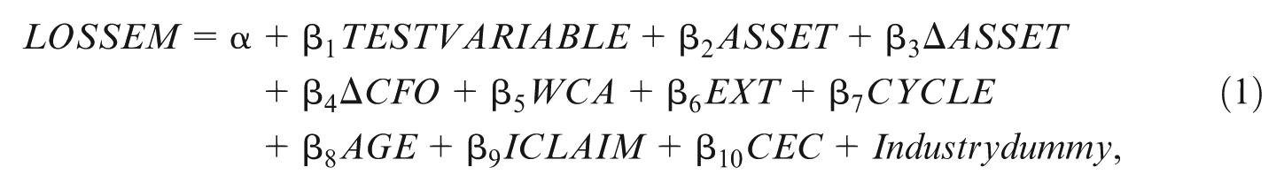
where LOSSEM = an indicator variable that takes the value of 1 if the firm has scaled earnings in the interval between 0 (inclusive) and 0.0028 (exclusive), and 0 if the firm has scaled earnings in the interval between −0.0028 (inclusive) and 0 (exclusive); TESTVARIABLE = TAXCOST: marginal tax rates based on the method of Gramlich et al. (2004); ASSET = natural log of total assets at the end of the fiscal year; ΔASSET = first difference in total assets, divided by total assets at the end of the previous year; ΔCFO = first difference in cash flows, divided by total assets at the end of the previous year; WCA = working capital accruals, divided by total assets at the end of the previous year; EXT = extraordinary items, divided by total assets at the end of the previous year; CYCLE = the natural log of the length of the operating cycle in days; AGE = the natural log of the firm age; ICLAIM = the reliance on implicit claims, computed using principal component analysis; CEC = the change in executive compensations (total cash salary and total bonus paid to all directors) divided by the change in net income; Industry dummy = industry dummy variables.
In accordance with many prior studies, we focus on firms that report small profits or losses to grasp earnings management to avoid losses (Beatty, Ke, & Petroni, 2002; Burgstahler et al., 2006; Leuz et al., 2003). Specifically, this analysis investigates the level of scaled earnings within two intervals, one between −0.0028 (inclusive) and 0 (exclusive) and the other between 0 (inclusive) and 0.0028 (exclusive). In constructing the histograms, based on the formula used in previous studies (Beatty et al., 2002; Degeorge, Patel, & Zeckhauser, 1999), we use a bin width of twice the interquartile range of the variable multiplied by the negative cube root of the sample size. The formula indicates that the bin width in our histogram is 0.0014. 10 Consequently, following the procedure of Beatty et al. (2002), we use an interval size twice the bin width used in the histogram. 11
In the regression model (Equation 1), the coefficient of TESTVARIABLE (i.e., TAXCOST) measures the relationship between incentive for tax management and the discontinuity of earnings distribution around zero. If the relationship is consistent with the prediction of H1, the coefficient of TAXCOST should be positive. Furthermore, we use some control variables to explain the discontinuity of earnings distribution based on the findings of previous studies. In particular, following the model of Beatty et al. (2002), we control for firm size (ASSET), growth (ΔASSET), and profitability (ΔCFO). If higher growth and larger firms are increasingly more profitable or more likely to manage earnings to avoid earnings losses, the coefficients of ΔASSET and ASSET should be positive. We also expect a firm with greater profits to be more likely to report small earnings rather than small losses. Therefore, we expect the coefficients of ΔCFO to be positive.
Working capital accruals (WCA) and extraordinary items (EXT) are included in the model to control for the effect of discretionary accounting choices. Because working capital accruals and extraordinary items are likely to be used to manage earnings to avoid losses, the coefficients of these two variables are expected to be positive. Burgstahler et al. (2006) contend that the length of the operating cycle in days (CYCLE) and the number of years since incorporation (AGE) have to be controlled, because these variables are likely to be associated with the level of earnings management and variation between privately held and public firms. Finally, compensation earnings coefficients (CEC) included in the model to control the effect of managerial incentive intensity. We expect that these variables are positively associated with the incidence of earnings management.
Finally, we control for a firm’s implicit claims with its stakeholders (ICLAIM) because prior studies argued that managers’ incentive to beat earnings benchmarks through earnings management is stronger for firms that rely heavily on implicit claims (Bowen, DuCharme, & Shores, 1995; Matsumoto, 2002). The coefficient of ICLAIM is expected to be positive. 12
To test H2, we investigate the effect of the strength of the relationship between the firm and its bank on the discontinuity of earnings distribution. We use the following FIN variable as a TESTVARIABLE:
FIN = the strength of the relationship between firm and their bank, computed using principal component analysis.
We expect that the coefficient of FIN will be positive if the relationship between FIN and LOSSEM is consistent with the prediction of H2.
Research models for testing H3 and H4
Before testing H3 and H4, to test our basic assumption, we examine the relationship between loss-avoidance tendency and the difference between public and private firms. In particular, we insert the PRIVATE variable as a TESTVARIABLE.
PRIVATE = an indicator variable that takes the value of 1 if the firm is unlisted, and 0 otherwise.
In our hypotheses development, we assume that private firms have greater incentive to report slightly positive earnings than do public firms. Thus, the coefficient of PRIVATE is expected to be positive based on our prediction.
To test H3 and H4, we examine the effect of the difference between public and private firms on the relationship between institutional features (i.e., tax-management incentive and the relationship with bank) and loss-avoidance incentive. We add interaction terms for PRIVATE and TAXCOST (FIN) in regression models to test the hypotheses. Thus, TESTVARIABLE are TAXCOST and PRIVATE×TAXCOST (FIN and PRIVATE×FIN). H3 and H4 predict that loss-avoidance incentives due to these institutional features are greater for private firms. Thus, the sign of these interaction variables (i.e., PRIVATE×TAXCOST and PRIVATE×FIN) is predicted to be positive. 13
Sample Selection and Descriptive Statistic
Sample Selection
Our sample selection procedure is summarized in Table 1. The initial sample included public and private firms for the period 1979-2007 after excluding financial institutions and other financial institutions. Public firms are defined as firms listed on at least one of the eight stock exchanges or traded on the over-the-counter market in Japan. We define private firms as stock companies unlisted on any of the stock exchanges or traded on the over-the-counter market in Japan. More specifically, to be included in our sample of private firms, a firm must satisfy any of the following requirements: (a) the amount of stated capital (shihon kin) on the balance sheet as of the end of the most recent business year is 500 million yen or more or (b) the total sum of the amounts in the liabilities section of the balance sheet as of the end of the most recent business year is 20 billion yen or more. 14
Sample Selection Procedure.
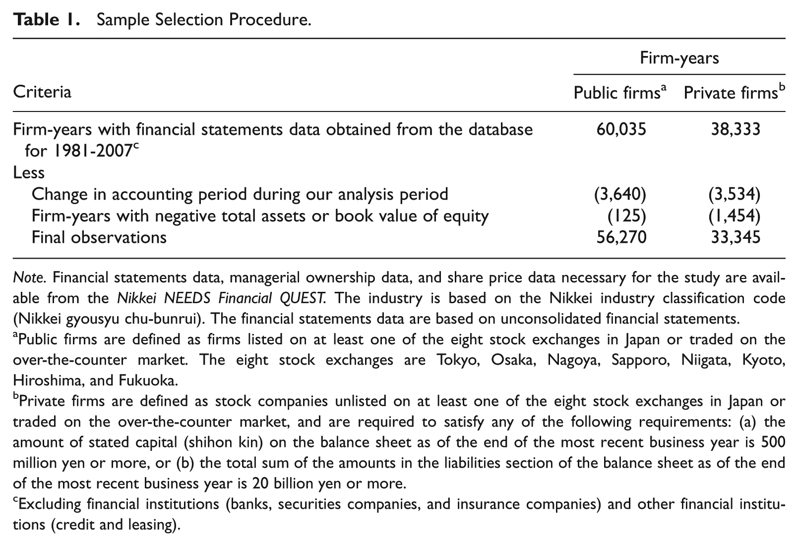
Note. Financial statements data, managerial ownership data, and share price data necessary for the study are available from the Nikkei NEEDS Financial QUEST. The industry is based on the Nikkei industry classification code (Nikkei gyousyu chu-bunrui). The financial statements data are based on unconsolidated financial statements.
Public firms are defined as firms listed on at least one of the eight stock exchanges in Japan or traded on the over-the-counter market. The eight stock exchanges are Tokyo, Osaka, Nagoya, Sapporo, Niigata, Kyoto, Hiroshima, and Fukuoka.
Private firms are defined as stock companies unlisted on at least one of the eight stock exchanges in Japan or traded on the over-the-counter market, and are required to satisfy any of the following requirements: (a) the amount of stated capital (shihon kin) on the balance sheet as of the end of the most recent business year is 500 million yen or more, or (b) the total sum of the amounts in the liabilities section of the balance sheet as of the end of the most recent business year is 20 billion yen or more.
Excluding financial institutions (banks, securities companies, and insurance companies) and other financial institutions (credit and leasing).
Under the Japanese Companies Act, private firms are required to prepare financial statements in accordance with corporate accounting customs, or GAAP (Companies Act, Article 431). In practice, most private firms that meet the above requirements (i.e., our sample firms) prepare their financial statements following the accounting standards for listed companies. 15 Thus, for our sample, we can reasonably compare the financial data of listed firms and unlisted firms without bias due to differences in the accounting standards.
We obtained our initial sample of 98,368 observations (60,035 for public firms observations and 38,333 for private firms) of unconsolidated financial statement data from the Nikkei NEEDS Financial QUEST for 1979-2007. 16 We use the accounting data from unconsolidated financial statement because our main hypotheses deal with managerial incentives for tax management, and taxable income is generally calculated on the basis of unconsolidated accounting earnings in Japan.
We deleted firms whose accounting period changed during our analytical period; this resulted in 56,395 public and 34,799 private firm observations. Finally, we excluded observations with negative total assets or a negative book value of equity. The final sample consists of 56,270 public and 33,345 private firm observations.
Descriptive Statistics
Table 2 reports the descriptive statistics of earnings variables for earnings distribution analysis. The table shows that public firms are more profitable than private firms in general. Although the average value of the level of net income for public firms is 0.022 for our sample period, the average value of private firms is 0.013. Table 3 summarizes the descriptive statistics of the variables for our regression analysis in which we focus on firms reporting slight profits or losses to test the hypotheses. The fact that the LOSSEM dummy variable is 0.880 indicates that 88% of observations in our sample report positive earnings. This clear contrast between profit and loss firms around zero earnings is consistent with the findings of prior studies examining earnings distribution for Japanese firms.
Descriptive Statistics on Earnings.
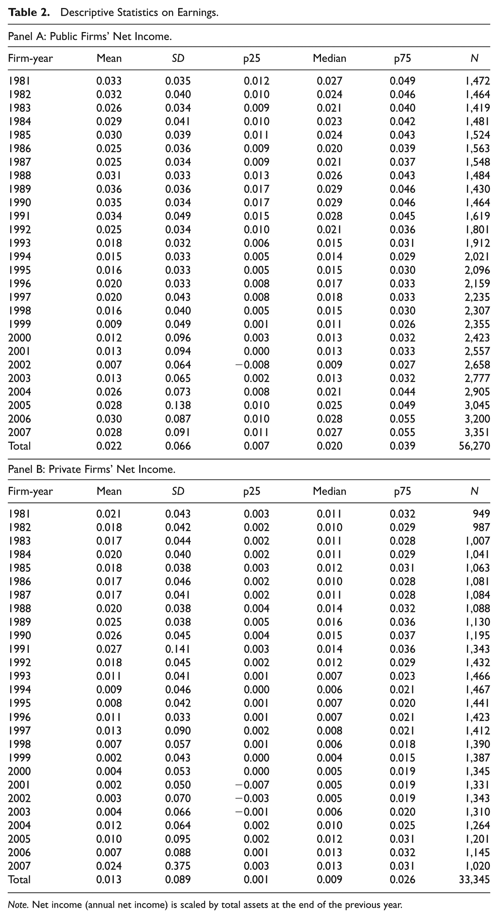
Note. Net income (annual net income) is scaled by total assets at the end of the previous year.
Descriptive Statistics on the Variables for Our Regression Analysis.
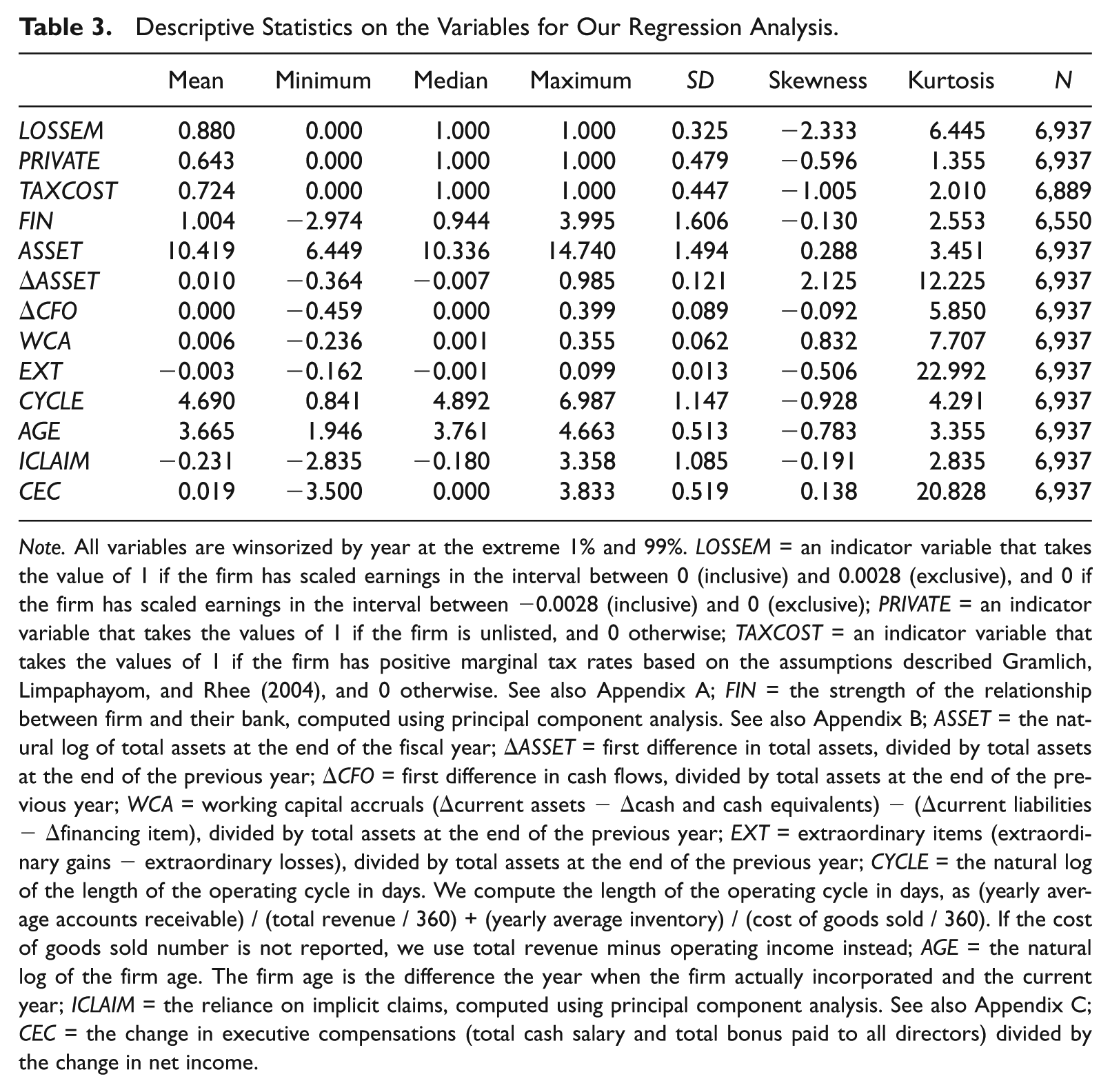
Note. All variables are winsorized by year at the extreme 1% and 99%. LOSSEM = an indicator variable that takes the value of 1 if the firm has scaled earnings in the interval between 0 (inclusive) and 0.0028 (exclusive), and 0 if the firm has scaled earnings in the interval between −0.0028 (inclusive) and 0 (exclusive); PRIVATE = an indicator variable that takes the values of 1 if the firm is unlisted, and 0 otherwise; TAXCOST = an indicator variable that takes the values of 1 if the firm has positive marginal tax rates based on the assumptions described Gramlich, Limpaphayom, and Rhee (2004), and 0 otherwise. See also Appendix A; FIN = the strength of the relationship between firm and their bank, computed using principal component analysis. See also Appendix B; ASSET = the natural log of total assets at the end of the fiscal year; ΔASSET = first difference in total assets, divided by total assets at the end of the previous year; ΔCFO = first difference in cash flows, divided by total assets at the end of the previous year; WCA = working capital accruals (Δcurrent assets −Δcash and cash equivalents) − (Δcurrent liabilities −Δfinancing item), divided by total assets at the end of the previous year; EXT = extraordinary items (extraordinary gains − extraordinary losses), divided by total assets at the end of the previous year; CYCLE = the natural log of the length of the operating cycle in days. We compute the length of the operating cycle in days, as (yearly average accounts receivable) / (total revenue / 360) + (yearly average inventory) / (cost of goods sold / 360). If the cost of goods sold number is not reported, we use total revenue minus operating income instead; AGE = the natural log of the firm age. The firm age is the difference the year when the firm actually incorporated and the current year; ICLAIM = the reliance on implicit claims, computed using principal component analysis. See also Appendix C; CEC = the change in executive compensations (total cash salary and total bonus paid to all directors) divided by the change in net income.
Furthermore, the table shows that the PRIVATE dummy variable is 0.643, which means that 64.3% of sample firms are private firms. We identify again that the ratio of private firms in our initial sample in Table 1 was only about 38% (i.e., the number of private firms was 38,333, and the total initial sample was 98,688 firms). It should be noted that the ratio clearly increases from initial sample to subsample with slight earnings, which suggests that observations of private firms are more concentrated around zero earnings.
Table 4 reveals the correlation matrix among the variables used in our regression models. The upper-right-hand portion of the table reports the Spearman rank-order correlations, and the lower-left-hand portion presents the Pearson correlations. In both correlation analyses, both TAXCOST and FIN are significantly and positively associated with LOSSEM. The results suggest that earnings management for loss avoidance increases as tax-management incentive and the bank dependency of firms increase, respectively, as hypothesized.
Correlations Matrix Among the Variables for Our Regression Analysis.
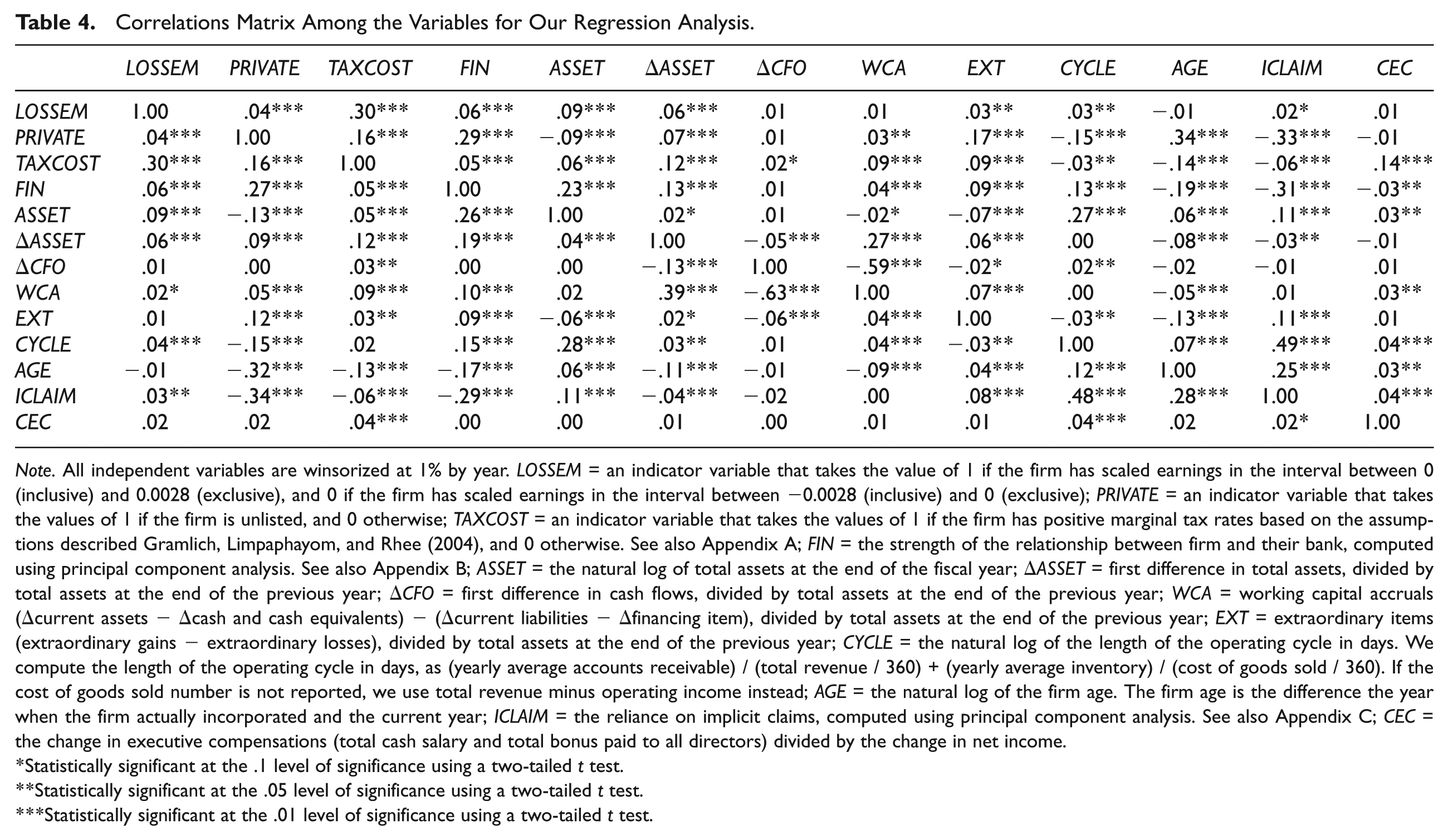
Note. All independent variables are winsorized at 1% by year. LOSSEM = an indicator variable that takes the value of 1 if the firm has scaled earnings in the interval between 0 (inclusive) and 0.0028 (exclusive), and 0 if the firm has scaled earnings in the interval between −0.0028 (inclusive) and 0 (exclusive); PRIVATE = an indicator variable that takes the values of 1 if the firm is unlisted, and 0 otherwise; TAXCOST = an indicator variable that takes the values of 1 if the firm has positive marginal tax rates based on the assumptions described Gramlich, Limpaphayom, and Rhee (2004), and 0 otherwise. See also Appendix A; FIN = the strength of the relationship between firm and their bank, computed using principal component analysis. See also Appendix B; ASSET = the natural log of total assets at the end of the fiscal year; ΔASSET = first difference in total assets, divided by total assets at the end of the previous year; ΔCFO = first difference in cash flows, divided by total assets at the end of the previous year; WCA = working capital accruals (Δcurrent assets −Δcash and cash equivalents) − (Δcurrent liabilities −Δfinancing item), divided by total assets at the end of the previous year; EXT = extraordinary items (extraordinary gains − extraordinary losses), divided by total assets at the end of the previous year; CYCLE = the natural log of the length of the operating cycle in days. We compute the length of the operating cycle in days, as (yearly average accounts receivable) / (total revenue / 360) + (yearly average inventory) / (cost of goods sold / 360). If the cost of goods sold number is not reported, we use total revenue minus operating income instead; AGE = the natural log of the firm age. The firm age is the difference the year when the firm actually incorporated and the current year; ICLAIM = the reliance on implicit claims, computed using principal component analysis. See also Appendix C; CEC = the change in executive compensations (total cash salary and total bonus paid to all directors) divided by the change in net income.
Statistically significant at the .1 level of significance using a two-tailed t test.
Statistically significant at the .05 level of significance using a two-tailed t test.
Statistically significant at the .01 level of significance using a two-tailed t test.
Results
Preliminary Analysis
First, we observe the earnings distribution in Japanese firms as a preliminary analysis. Figure 1 compares the distributions of the scaled net income for public firms (Panel A) and private firms (Panel B). Consistent with the findings of prior studies, both panels show drastic discontinuities at zero in the distribution of scaled net income in Japanese firms, which suggests that Japanese firm managers have strong incentive to avoid earnings losses, given the assumption of general earnings management research.
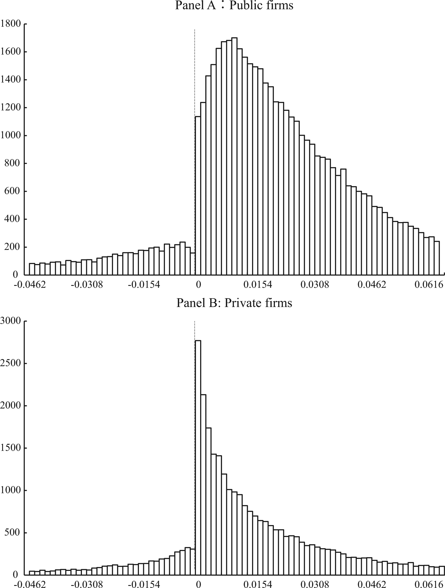
The distribution of the scaled annual net income.
Table 5 summarizes the standardized differences and the earnings management ratio (EM ratio) in the distributions. The standardized differences are used to test the significance of the irregularities near zero earnings through a statistical test based on Burgstahler and Dichev (1997). 17 The EM ratio is defined as the number of observations in the interval to the immediate right of (and including) 0 divided by the number of observations in the interval to the immediate left of 0 (Beatty et al., 2002; Brown & Caylor, 2005; Dechow, Richardson, & Tuna, 2003). We use this ratio to test for differences in the degree of discontinuities around zero between public and private firms’ earnings distributions.
Standardized Differences and EM Ratio.
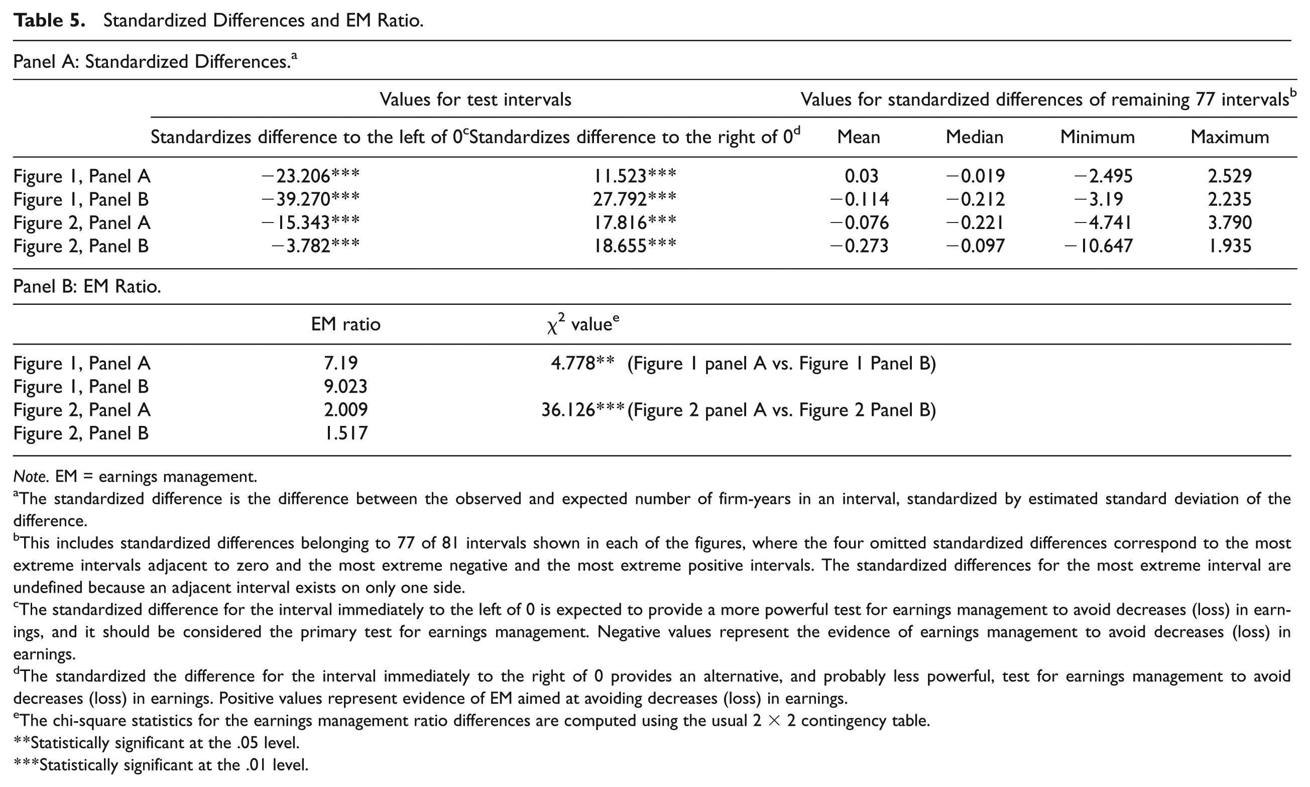
Note. EM = earnings management.
The standardized difference is the difference between the observed and expected number of firm-years in an interval, standardized by estimated standard deviation of the difference.
This includes standardized differences belonging to 77 of 81 intervals shown in each of the figures, where the four omitted standardized differences correspond to the most extreme intervals adjacent to zero and the most extreme negative and the most extreme positive intervals. The standardized differences for the most extreme interval are undefined because an adjacent interval exists on only one side.
The standardized difference for the interval immediately to the left of 0 is expected to provide a more powerful test for earnings management to avoid decreases (loss) in earnings, and it should be considered the primary test for earnings management. Negative values represent the evidence of earnings management to avoid decreases (loss) in earnings.
The standardized the difference for the interval immediately to the right of 0 provides an alternative, and probably less powerful, test for earnings management to avoid decreases (loss) in earnings. Positive values represent evidence of EM aimed at avoiding decreases (loss) in earnings.
The chi-square statistics for the earnings management ratio differences are computed using the usual 2 × 2 contingency table.
Statistically significant at the .05 level.
Statistically significant at the .01 level.
The tests of standardized differences indicate that the irregularities near zero earnings are statistically significant in both panels. A chi-square test on EM ratios indicates that the EM ratio of private firms, 9.023, is significantly higher than the ratio of public firms, 7.190. These results suggest that Japanese managers of both public and private firms have strong incentive to avoid losses, and the degree of earnings management, that is, the degree of discontinuity of earnings distribution, is more pervasive for private firms than public firms.
Finally, we also present the distribution of the changes in net income to compare with the results for the distribution of the levels of net income. During hypotheses development, we assumed that the institutional factors on which we focus in this study induce managers to report slightly positive earnings, and that such incentives are stronger for private firms than for public firms. The reason for expecting salient earnings management in private firms in particular is that capital market pressure and the related earnings management incentive are absent for private firms. Furthermore, Coppens and Peek (2005) argued and provided evidence suggesting that earnings management to avoid earnings decreases is due to capital market pressure. Consequently, given that the two institutional factors we examine here create stronger incentive for earnings management in private firms, and that the incentive for avoiding earnings decreases is due to capital market pressure, we expect earnings management to avoid decreases to be less pervasive for private firms than for public firms.
The results of Figure 2 are consistent with this prediction. The figure shows that although there are salient irregularities at zero in the distribution of earnings changes for public firms (Panel A), the irregularities in the earnings distribution for private firms (Panel B) is less clear. The statistical tests of Table 5 also confirm difference in irregularities near zero between the two distributions. The table indicates that the EM ratio of private firms is significantly lower than that of public firms, which suggest that managers of private firms do not have as much incentive to avoid decreases in earnings as the managers of public firms, and the incentive for earnings management to avoid decreases is due to capital market pressure.
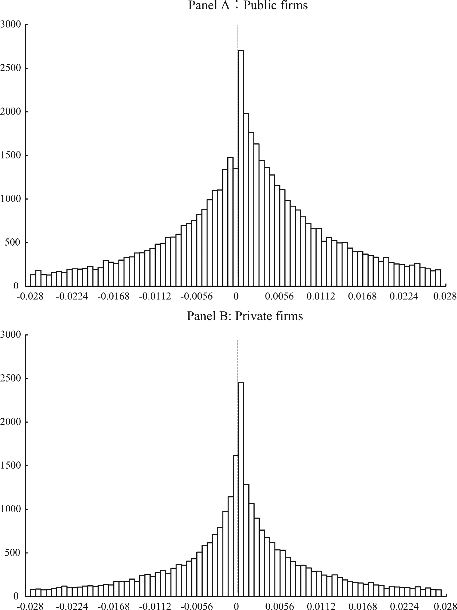
The distribution of scaled changes in the annual net income.
Our overall results on preliminary analyses are consistent with the theoretical background of our hypotheses and the findings of prior studies on the following points. First, there are drastic irregularities near zero in the distribution of the level of earnings in Japanese firms, which is the basic assumption behind our primary concern, and is consistent with the findings of prior studies (Shuto, 2009; Suda & Shuto, 2007; Thomas et al., 2004). Second, the irregularities in the distribution of the level of earnings are more pervasive for private firms than for public firms. Finally, the irregularities in the distribution of the changes in earnings are less pervasive for private firms than for public firms. The latter two findings partially support our discussion during hypotheses development, suggesting that the irregularities in the distribution of the level of earnings are mainly due to incentives for tax avoidance and maintaining good relationships with banks.
Main Results
Results for H1 and H2
To test H1, we estimate regression model (Equation 1) using pooled regressions and reported t statistics based on standard errors clustered at firm and year levels following Petersen’s (2009) analyses. 18
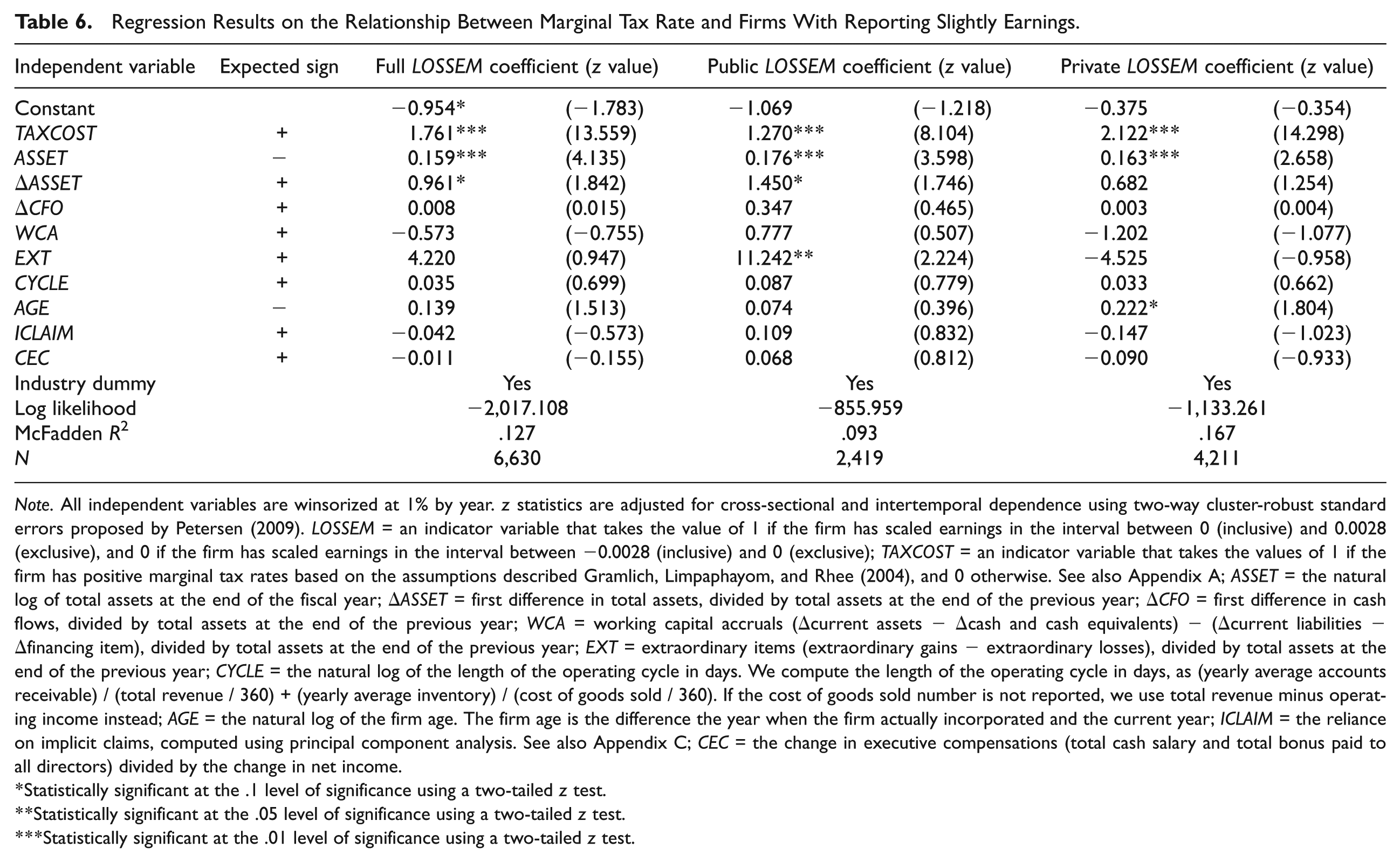
Table 6 summarizes the regression results for the full sample, public firms, and private firms, respectively. In column 3 of Table 6, the regression result for the full sample shows that the coefficient of TAXCOST, 1.761, is significantly positive at the 1% level, as expected. We also find that the coefficients of TAXCOST in regression models for public firms (column 4) and private firms (column 5) are also both significantly positive at the 1% level. These results are in accordance with H1, suggesting that there are greater irregularities in the distribution of the level of earnings as marginal tax rate increases. In other words, firms with a higher marginal tax rate are more likely to engage in earnings management to report slightly positive earnings.
Regression Results on the Relationship Between Marginal Tax Rate and Firms With Reporting Slightly Earnings.
Note. All independent variables are winsorized at 1% by year. z statistics are adjusted for cross-sectional and intertemporal dependence using two-way cluster-robust standard errors proposed by Petersen (2009). LOSSEM = an indicator variable that takes the value of 1 if the firm has scaled earnings in the interval between 0 (inclusive) and 0.0028 (exclusive), and 0 if the firm has scaled earnings in the interval between −0.0028 (inclusive) and 0 (exclusive); TAXCOST = an indicator variable that takes the values of 1 if the firm has positive marginal tax rates based on the assumptions described Gramlich, Limpaphayom, and Rhee (2004), and 0 otherwise. See also Appendix A; ASSET = the natural log of total assets at the end of the fiscal year; ΔASSET = first difference in total assets, divided by total assets at the end of the previous year; ΔCFO = first difference in cash flows, divided by total assets at the end of the previous year; WCA = working capital accruals (Δcurrent assets −Δcash and cash equivalents) − (Δcurrent liabilities −Δfinancing item), divided by total assets at the end of the previous year; EXT = extraordinary items (extraordinary gains − extraordinary losses), divided by total assets at the end of the previous year; CYCLE = the natural log of the length of the operating cycle in days. We compute the length of the operating cycle in days, as (yearly average accounts receivable) / (total revenue / 360) + (yearly average inventory) / (cost of goods sold / 360). If the cost of goods sold number is not reported, we use total revenue minus operating income instead; AGE = the natural log of the firm age. The firm age is the difference the year when the firm actually incorporated and the current year; ICLAIM = the reliance on implicit claims, computed using principal component analysis. See also Appendix C; CEC = the change in executive compensations (total cash salary and total bonus paid to all directors) divided by the change in net income.
Statistically significant at the .1 level of significance using a two-tailed z test.
Statistically significant at the .05 level of significance using a two-tailed z test.
Statistically significant at the .01 level of significance using a two-tailed z test.
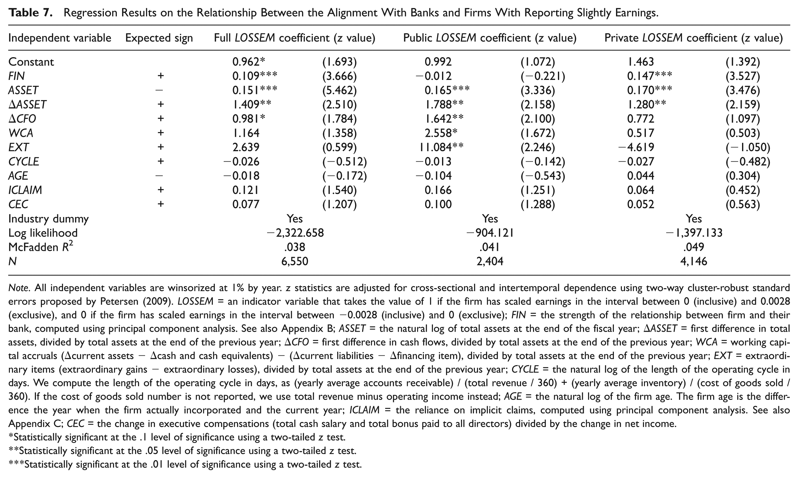
The regression results of model for H2 are reported in Table 7. Column 3 in the table indicates that FIN is significantly and positively associated with LOSSEM at the 1% level for the full sample, which is consistent with H2. In columns 4 and 5 of the table, contrasting results for the FIN variables for public and private firms are presented. For the private firm sample, the coefficient of FIN is significantly positive at the 1% level, as expected, but the coefficient of FIN is negative and not significant for the public firm sample. It is likely that the incentive of maintaining alignment with the bank is stronger for managers of private firms than for managers of public firms, consistent with our prediction. With respect to control variables in the regression model for the full sample, we find that larger firms, higher growth firms, and firms with greater profits tend to report slightly positive earnings more often.
Regression Results on the Relationship Between the Alignment With Banks and Firms With Reporting Slightly Earnings.
Note. All independent variables are winsorized at 1% by year. z statistics are adjusted for cross-sectional and intertemporal dependence using two-way cluster-robust standard errors proposed by Petersen (2009). LOSSEM = an indicator variable that takes the value of 1 if the firm has scaled earnings in the interval between 0 (inclusive) and 0.0028 (exclusive), and 0 if the firm has scaled earnings in the interval between −0.0028 (inclusive) and 0 (exclusive); FIN = the strength of the relationship between firm and their bank, computed using principal component analysis. See also Appendix B; ASSET = the natural log of total assets at the end of the fiscal year; ΔASSET = first difference in total assets, divided by total assets at the end of the previous year; ΔCFO = first difference in cash flows, divided by total assets at the end of the previous year; WCA = working capital accruals (Δcurrent assets −Δcash and cash equivalents) − (Δcurrent liabilities −Δfinancing item), divided by total assets at the end of the previous year; EXT = extraordinary items (extraordinary gains − extraordinary losses), divided by total assets at the end of the previous year; CYCLE = the natural log of the length of the operating cycle in days. We compute the length of the operating cycle in days, as (yearly average accounts receivable) / (total revenue / 360) + (yearly average inventory) / (cost of goods sold / 360). If the cost of goods sold number is not reported, we use total revenue minus operating income instead; AGE = the natural log of the firm age. The firm age is the difference the year when the firm actually incorporated and the current year; ICLAIM = the reliance on implicit claims, computed using principal component analysis. See also Appendix C; CEC = the change in executive compensations (total cash salary and total bonus paid to all directors) divided by the change in net income.
Statistically significant at the .1 level of significance using a two-tailed z test.
Statistically significant at the .05 level of significance using a two-tailed z test.
Statistically significant at the .01 level of significance using a two-tailed z test.
Results for H3 and H4
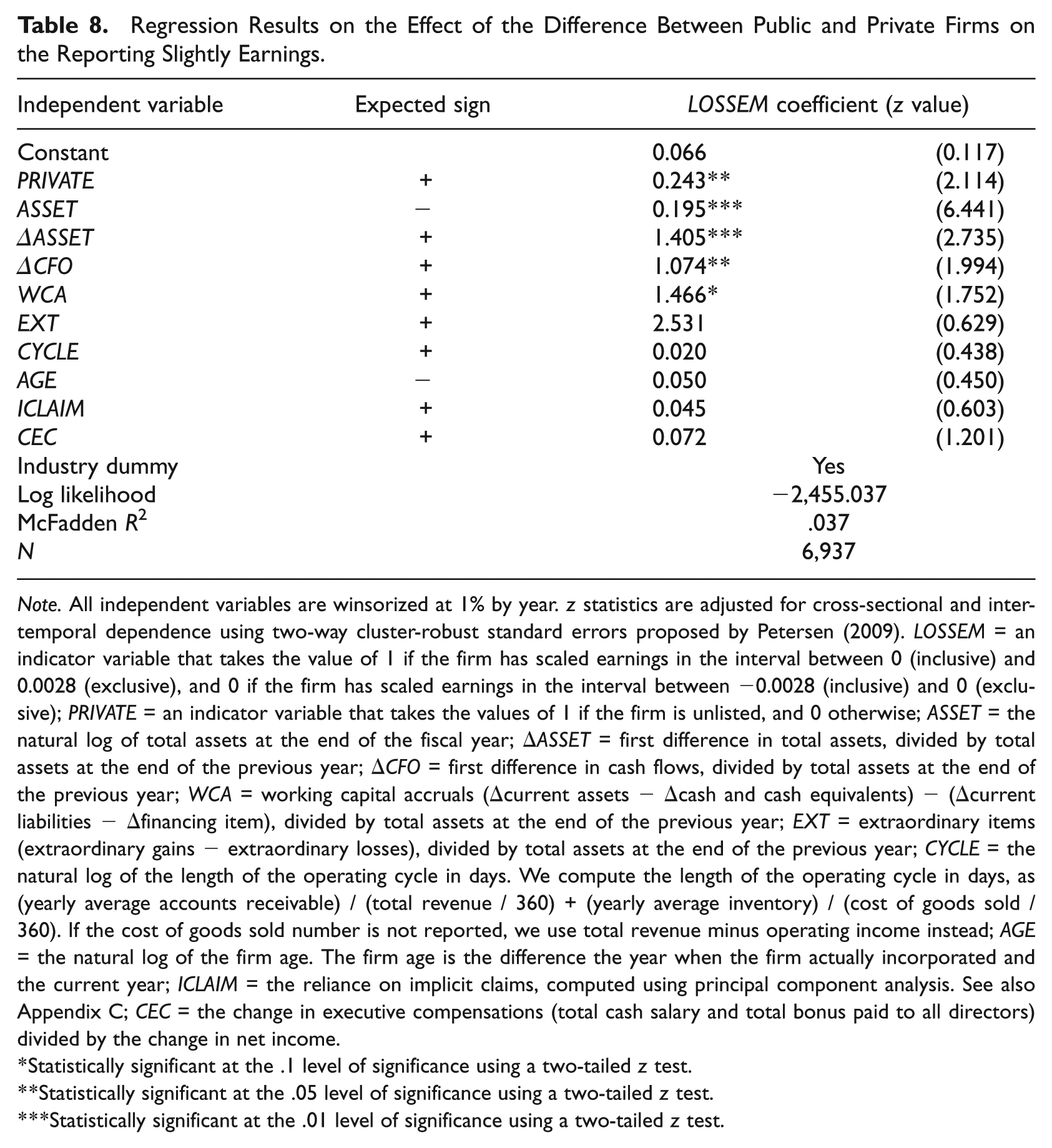
Before testing the hypotheses, Table 8 presents the results for regression model, which examines the relationship between the difference between public and private firms and loss-avoidance incentives. In Table 8, the coefficient of PRIVATE, 0.243, is significantly positive. Private firms are more likely to report slightly positive earnings than public firms. The results are in accordance with the findings of preliminary analysis and again support our assumption.
Regression Results on the Effect of the Difference Between Public and Private Firms on the Reporting Slightly Earnings.
Note. All independent variables are winsorized at 1% by year. z statistics are adjusted for cross-sectional and intertemporal dependence using two-way cluster-robust standard errors proposed by Petersen (2009). LOSSEM = an indicator variable that takes the value of 1 if the firm has scaled earnings in the interval between 0 (inclusive) and 0.0028 (exclusive), and 0 if the firm has scaled earnings in the interval between −0.0028 (inclusive) and 0 (exclusive); PRIVATE = an indicator variable that takes the values of 1 if the firm is unlisted, and 0 otherwise; ASSET = the natural log of total assets at the end of the fiscal year; ΔASSET = first difference in total assets, divided by total assets at the end of the previous year; ΔCFO = first difference in cash flows, divided by total assets at the end of the previous year; WCA = working capital accruals (Δcurrent assets −Δcash and cash equivalents) − (Δcurrent liabilities −Δfinancing item), divided by total assets at the end of the previous year; EXT = extraordinary items (extraordinary gains − extraordinary losses), divided by total assets at the end of the previous year; CYCLE = the natural log of the length of the operating cycle in days. We compute the length of the operating cycle in days, as (yearly average accounts receivable) / (total revenue / 360) + (yearly average inventory) / (cost of goods sold / 360). If the cost of goods sold number is not reported, we use total revenue minus operating income instead; AGE = the natural log of the firm age. The firm age is the difference the year when the firm actually incorporated and the current year; ICLAIM = the reliance on implicit claims, computed using principal component analysis. See also Appendix C; CEC = the change in executive compensations (total cash salary and total bonus paid to all directors) divided by the change in net income.
Statistically significant at the .1 level of significance using a two-tailed z test.
Statistically significant at the .05 level of significance using a two-tailed z test.
Statistically significant at the .01 level of significance using a two-tailed z test.
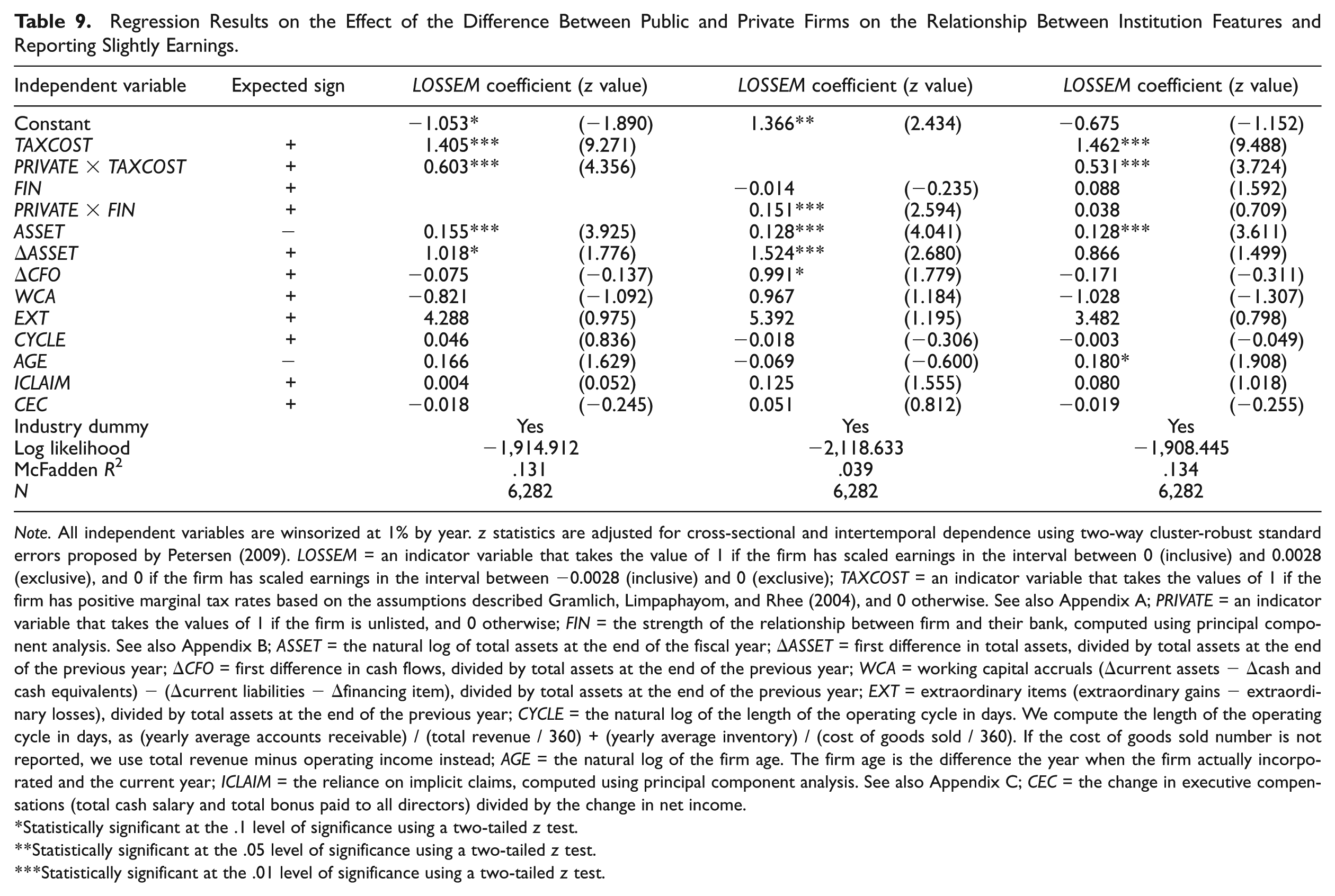
Next, to test the hypotheses, we examine the effect of the difference between public and private firms on the relationship between the institutional factor and reporting slightly positive earnings. Table 9 summarizes the results for regression models in testing H3 and H4. The result of regression model on H3 is reported in column 3 of Table 9. Consistent with H3, the coefficient of PRIVATE×TAXCOST is significantly positive at the 1% level. This finding means that the marginal tax rate is more associated with the loss-avoidance tendency for private firms than for public firms. Furthermore, column 4 of the table reveals the results of regression model on H4, showing that PRIVATE×FIN has a significantly positive coefficient, as hypothesized. The result suggests that the relationship between the degree of a firm’s bank dependence and the loss-avoidance tendency is higher for private firms.
Regression Results on the Effect of the Difference Between Public and Private Firms on the Relationship Between Institution Features and Reporting Slightly Earnings.
Note. All independent variables are winsorized at 1% by year. z statistics are adjusted for cross-sectional and intertemporal dependence using two-way cluster-robust standard errors proposed by Petersen (2009). LOSSEM = an indicator variable that takes the value of 1 if the firm has scaled earnings in the interval between 0 (inclusive) and 0.0028 (exclusive), and 0 if the firm has scaled earnings in the interval between −0.0028 (inclusive) and 0 (exclusive); TAXCOST = an indicator variable that takes the values of 1 if the firm has positive marginal tax rates based on the assumptions described Gramlich, Limpaphayom, and Rhee (2004), and 0 otherwise. See also Appendix A; PRIVATE = an indicator variable that takes the values of 1 if the firm is unlisted, and 0 otherwise; FIN = the strength of the relationship between firm and their bank, computed using principal component analysis. See also Appendix B; ASSET = the natural log of total assets at the end of the fiscal year; ΔASSET = first difference in total assets, divided by total assets at the end of the previous year; ΔCFO = first difference in cash flows, divided by total assets at the end of the previous year; WCA = working capital accruals (Δcurrent assets −Δcash and cash equivalents) − (Δcurrent liabilities −Δfinancing item), divided by total assets at the end of the previous year; EXT = extraordinary items (extraordinary gains − extraordinary losses), divided by total assets at the end of the previous year; CYCLE = the natural log of the length of the operating cycle in days. We compute the length of the operating cycle in days, as (yearly average accounts receivable) / (total revenue / 360) + (yearly average inventory) / (cost of goods sold / 360). If the cost of goods sold number is not reported, we use total revenue minus operating income instead; AGE = the natural log of the firm age. The firm age is the difference the year when the firm actually incorporated and the current year; ICLAIM = the reliance on implicit claims, computed using principal component analysis. See also Appendix C; CEC = the change in executive compensations (total cash salary and total bonus paid to all directors) divided by the change in net income.
Statistically significant at the .1 level of significance using a two-tailed z test.
Statistically significant at the .05 level of significance using a two-tailed z test.
Statistically significant at the .01 level of significance using a two-tailed z test.
Finally, we include the two interaction terms in the model simultaneously; the result is reported in column 5 of Table 9. The table indicates that although PRIVATE×TAXCOST has a significantly positive coefficient at the 1% level, the coefficient of PRIVATE×FIN is positive but not significant. This evidence suggests that the incentive for tax avoidance has a higher impact on the loss-avoidance tendency of private firms.
Additional Analysis
In this section, we conduct additional analysis on our earnings distribution research method. Although many studies that follow Burgstahler and Dichev (1997) attribute the discontinuity of earnings distribution around zero to earnings management, recent studies question whether this discontinuity is evidence of earnings management by firm managers. For example, Durtschi and Easton (2005, 2009) contend that the finding may be the result of (a) the scaling effect on variables or (b) selection biases in the sample. In particular, first, they assert that the deflators for small-loss firms are systematically lower than the corresponding figures for small-profit firms, which may induce a discontinuity in scaled earnings around zero. Second, they argue that a larger portion of loss firms do not have a beginning-of-period market capitalization—a common deflator used in prior studies 19 —possibly resulting in selection biases that may cause a discontinuity in the earnings distribution around zero.
A useful way to address this issue is to reexamine our analyses based on unscaled earnings (Burgstahler & Chuk, 2013; Jacob & Jorgensen, 2007). In particular, we adopt the research method of Burgstahler and Chuk (2013) because of its significant advantage in enabling an examination of unscaled net income. Although an analysis based on unscaled earnings may resolve the problem indicated by Durtschi and Easton (2005, 2009), a related problem is that the analysis does not account for (a) the strong relationship between firm size and earnings and (b) size-related differences in earnings management. The approach by Burgstahler and Chuk (2013) addresses these issues. Specifically, they examine the distributions of unscaled net income by partitioning the population based on size and using an interval width adjusted to reflected size-related differences in earnings management. 20
Following Burgstahler and Chuk (2013), first, we partition the population into quartiles based on firm size, that is, total assets. Second, we use an interval width of approximately 0.25% of the median total assets for the observations in each quartile-based subsample. Third, instead of using LOSSEM, as used in our main analysis, we use the USLOSSEM variable, an indicator variable that takes the value of 1 if the firm has unscaled earnings in the interval immediately above zero in histograms, and zero if the firm has unscaled earnings in the interval immediately below zero in histograms. Finally, we replicate the main analyses in Tables 6, 7, and 9 using the USLOSSEM variable.
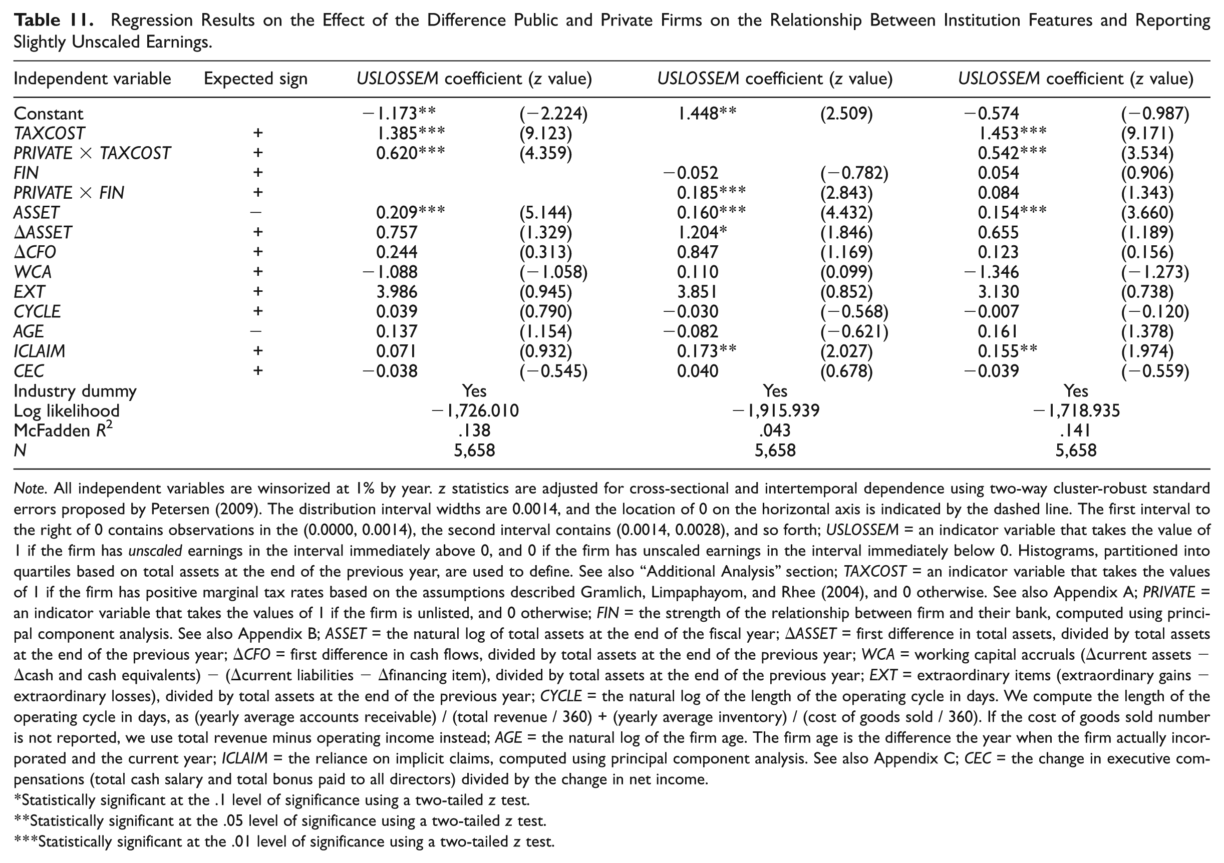
Table 10 summarizes the regression results on the relationship between marginal tax rate (the alignment with banks) and firms in the full sample that report slight earnings. The table shows that the coefficient on TAXCOST (FIN), 1.764 (0.086), is significantly positive at the 1% level, which is consistent with H1 and H2. Furthermore, Table 11 reveals the results of the effect of the difference between public and private firms on the relationship between the institutional factor and reporting slightly positive earnings (i.e., the replication analyses of Table 9 using USLOSSEM). Consistent with H3 and H4, the coefficient on PRIVATE×TAXCOST (PRIVATE×FIN), 0.620 (0.185), is significantly positive at the 1% level. Therefore, our results are robust under an additional test of the alternative earnings distribution approach.
Regression Results on the Relationship Between Marginal Tax Rate (the Alignment With Banks) and Firms With Reporting Slightly Unscaled Earnings.

Note. All independent variables are winsorized at 1% by year. z statistics are adjusted for cross-sectional and intertemporal dependence using two-way cluster-robust standard errors proposed by Petersen (2009). USLOSSEM = an indicator variable that takes the value of 1 if the firm has unscaled earnings in the interval immediately above 0, and 0 if the firm has unscaled earnings in the interval immediately below 0. Histograms, partitioned into quartiles based on total assets at the end of the previous year, are used to define. See also “Additional Analysis” section; TAXCOST = an indicator variable that takes the values of 1 if the firm has positive marginal tax rates based on the assumptions described Gramlich, Limpaphayom, and Rhee (2004), and 0 otherwise. See also Appendix A; FIN = the strength of the relationship between firm and their bank, computed using principal component analysis. See also Appendix B; ASSET = the natural log of total assets at the end of the fiscal year; ΔASSET = first difference in total assets, divided by total assets at the end of the previous year; ΔCFO = first difference in cash flows, divided by total assets at the end of the previous year; WCA = working capital accruals (Δcurrent assets −Δcash and cash equivalents) − (Δcurrent liabilities −Δfinancing item), divided by total assets at the end of the previous year; EXT = extraordinary items (extraordinary gains − extraordinary losses), divided by total assets at the end of the previous year; CYCLE = the natural log of the length of the operating cycle in days. We compute the length of the operating cycle in days, as (yearly average accounts receivable) / (total revenue / 360) + (yearly average inventory) / (cost of goods sold / 360). If the cost of goods sold number is not reported, we use total revenue minus operating income instead; AGE = the natural log of the firm age. The firm age is the difference the year when the firm actually incorporated and the current year; ICLAIM = the reliance on implicit claims, computed using principal component analysis. See also Appendix C; CEC = the change in executive compensations (total cash salary and total bonus paid to all directors) divided by the change in net income.
Statistically significant at the .1 level of significance using a two-tailed z test.
Statistically significant at the .05 level of significance using a two-tailed z test.
Statistically significant at the .01 level of significance using a two-tailed z test.
Regression Results on the Effect of the Difference Public and Private Firms on the Relationship Between Institution Features and Reporting Slightly Unscaled Earnings.
Note. All independent variables are winsorized at 1% by year. z statistics are adjusted for cross-sectional and intertemporal dependence using two-way cluster-robust standard errors proposed by Petersen (2009). The distribution interval widths are 0.0014, and the location of 0 on the horizontal axis is indicated by the dashed line. The first interval to the right of 0 contains observations in the (0.0000, 0.0014), the second interval contains (0.0014, 0.0028), and so forth; USLOSSEM = an indicator variable that takes the value of 1 if the firm has unscaled earnings in the interval immediately above 0, and 0 if the firm has unscaled earnings in the interval immediately below 0. Histograms, partitioned into quartiles based on total assets at the end of the previous year, are used to define. See also “Additional Analysis” section; TAXCOST = an indicator variable that takes the values of 1 if the firm has positive marginal tax rates based on the assumptions described Gramlich, Limpaphayom, and Rhee (2004), and 0 otherwise. See also Appendix A; PRIVATE = an indicator variable that takes the values of 1 if the firm is unlisted, and 0 otherwise; FIN = the strength of the relationship between firm and their bank, computed using principal component analysis. See also Appendix B; ASSET = the natural log of total assets at the end of the fiscal year; ΔASSET = first difference in total assets, divided by total assets at the end of the previous year; ΔCFO = first difference in cash flows, divided by total assets at the end of the previous year; WCA = working capital accruals (Δcurrent assets −Δcash and cash equivalents) − (Δcurrent liabilities −Δfinancing item), divided by total assets at the end of the previous year; EXT = extraordinary items (extraordinary gains − extraordinary losses), divided by total assets at the end of the previous year; CYCLE = the natural log of the length of the operating cycle in days. We compute the length of the operating cycle in days, as (yearly average accounts receivable) / (total revenue / 360) + (yearly average inventory) / (cost of goods sold / 360). If the cost of goods sold number is not reported, we use total revenue minus operating income instead; AGE = the natural log of the firm age. The firm age is the difference the year when the firm actually incorporated and the current year; ICLAIM = the reliance on implicit claims, computed using principal component analysis. See also Appendix C; CEC = the change in executive compensations (total cash salary and total bonus paid to all directors) divided by the change in net income.
Statistically significant at the .1 level of significance using a two-tailed z test.
Statistically significant at the .05 level of significance using a two-tailed z test.
Statistically significant at the .01 level of significance using a two-tailed z test.
Conclusion
The purpose of this study is to explore which factors shape the discontinuities in the earnings distribution of Japanese firms, because previous studies have revealed that there are clear discontinuities at zero in the distribution of earnings levels in Japanese firms. We predict that some institutional factors specific to Japanese firms cause the peculiar discontinuities at zero in the earnings distribution of Japanese firms. In particular, we focus on two institutional factors: (a) the alignment between financial and tax accounting and (b) the close relationship between firms and their banks.
Based on deeper consideration of the effect of institutional factors on financial reporting incentive, we hypothesize that these factors induce managers to report slightly positive earnings, creating discontinuities at zero in the distribution of earnings levels. First, we show that firms with higher marginal tax rates are more likely to conduct earnings management to report slightly positive earnings. The results suggest that managers with the incentive for tax management tend to manage earnings to reduce their tax cost.
Second, we provide evidence that firm managers with close relationships with their banks tend to engage in earnings management to avoid losses, because reporting losses can be a visible signal of bad performance that may cause intervention by the banks. Finally, we reveal that the relationship between these institutional factors and the loss-avoidance behaviors is stronger for private firms than for public firms, which is also consistent with our prediction. In summary, our results suggest that unique institutional features in Japan give rise to the discontinuities around zero of earnings distribution, and the result is more pervasive for private firms than public firms.
We build on the work of previous studies, mainly comparative studies in international settings, by providing evidence from a significant research setting in which there are features of both institutional factors and earnings distribution, based on deeper consideration during hypothesis development. An important implication of this study is that institutional factors can affect managers’ reporting incentive and shape the discontinuities around zero of earnings distribution. It might be beneficial for standard setters, tax authorities, and bankers to know that Japanese firms’ managers have strong incentive to report slightly positive earnings due to their institutional factors, and that the incentive is greater for managers of private firms.
Footnotes
Appendix A
Appendix B
Principal Component Analysis Results on Measuring Financial Institutions’ Relationships.
| Panel A: Principal Component Analysis for Public and Private Firm. |
|||
|---|---|---|---|
| Correlation matrix | DEBT | LOAN | LOAN5 |
| DEBT | 1.00 | .61*** | .56*** |
| LOAN | .44*** | 1.00 | .94*** |
| LOAN5 | .44*** | .94*** | 1.00 |
| Total variance explained | Eigenvalue | % of variance | Cumulative % |
| Component 1 | 2.248 | 74.9 | 74.9 |
| Component 2 | 0.690 | 23.0 | 97.9 |
| Component 3 | 0.062 | 2.1 | 100.0 |
| Principal components (eigenvectors) | Component 1 | Component 2 | Component 3 |
| DEBT | 0.446 | 0.895 | 0.006 |
| LOAN | 0.634 | −0.311 | −0.708 |
| LOAN5 | 0.632 | −0.320 | 0.706 |
| Panel B: Principal Component Analysis for Public Firm. |
|||
| Correlation matrix | DEBT | LOAN | LOAN5 |
| DEBT | 1.00 | .62*** | .56*** |
| LOAN | .45*** | 1.00 | .93*** |
| LOAN5 | .44*** | .92*** | 1.00 |
| Total variance explained | Eigenvalue | % of variance | Cumulative % |
| Component 1 | 2.241 | 74.7 | 74.7 |
| Component 2 | 0.680 | 22.7 | 97.4 |
| Component 3 | 0.079 | 2.7 | 100.0 |
| Principal components (eigenvectors) | Component 1 | Component 2 | Component 3 |
| DEBT | 0.453 | 0.891 | 0.012 |
| LOAN | 0.632 | −0.312 | −0.710 |
| LOAN5 | 0.629 | −0.329 | 0.704 |
| Panel C: Principal Component Analysis for Private Firm. |
|||
| Correlation matrix | DEBT | LOAN | LOAN5 |
| DEBT | 1.00 | .59*** | .57*** |
| LOAN | .48*** | 1.00 | .95*** |
| LOAN5 | .48*** | .94*** | 1.00 |
| Total variance explained | Eigenvalue | % of variance | Cumulative % |
| Component 1 | 2.297 | 76.6 | 76.6 |
| Component 2 | 0.647 | 21.6 | 98.1 |
| Component 3 | 0.056 | 1.9 | 100.0 |
| Principal components (eigenvectors) | Component 1 | Component 2 | Component 3 |
| DEBT | 0.462 | 0.887 | 0.001 |
| LOAN | 0.627 | −0.326 | −0.708 |
| LOAN5 | 0.627 | −0.328 | 0.707 |
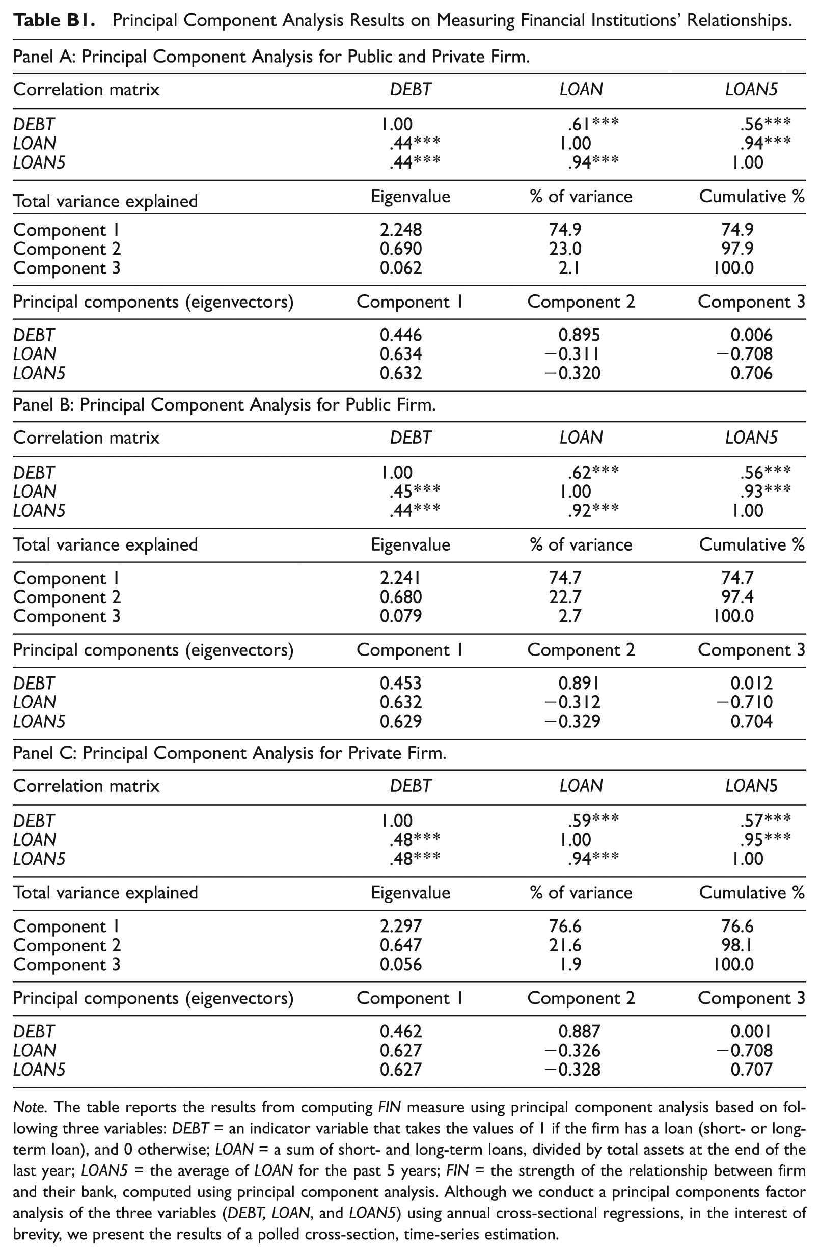
Note. The table reports the results from computing FIN measure using principal component analysis based on following three variables: DEBT = an indicator variable that takes the values of 1 if the firm has a loan (short- or long-term loan), and 0 otherwise; LOAN = a sum of short- and long-term loans, divided by total assets at the end of the last year; LOAN5 = the average of LOAN for the past 5 years; FIN = the strength of the relationship between firm and their bank, computed using principal component analysis. Although we conduct a principal components factor analysis of the three variables (DEBT, LOAN, and LOAN5) using annual cross-sectional regressions, in the interest of brevity, we present the results of a polled cross-section, time-series estimation.
Appendix C
Principal Component Analysis Results on Measuring Reliance on Implicit Claims.
| Panel A: Principal Component Analysis for Public and Private Firm. |
|||
|---|---|---|---|
| Correlation matrix | DUR | R&D | LABOR |
| DUR | 1.00 | .34*** | .13*** |
| R&D | .14*** | 1.00 | .08*** |
| LABOR | .20*** | .10*** | 1.00 |
| Total variance explained | Eigenvalue | % of variance | Cumulative % |
| Component 1 | 1.293 | 43.1 | 43.1 |
| Component 2 | 0.912 | 30.4 | 73.5 |
| Component 3 | 0.795 | 26.5 | 100.0 |
| Principal components (eigenvectors) | Component 1 | Component 2 | Component 3 |
| DUR | 0.636 | −0.174 | −0.752 |
| R&D | 0.497 | 0.838 | 0.226 |
| LABOR | 0.591 | −0.517 | 0.619 |
| Panel B: Principal Component Analysis for Public Firm. |
|||
| Correlation matrix | DUR | R&D | LABOR |
| DUR | 1.00 | .29*** | .05*** |
| R&D | .10*** | 1.00 | −.02*** |
| LABOR | .10*** | .04*** | 1.00 |
| Total variance explained | Eigenvalue | % of variance | Cumulative % |
| Component 1 | 1.161 | 38.7 | 38.7 |
| Component 2 | 0.958 | 31.9 | 70.6 |
| Component 3 | 0.882 | 29.4 | 100.0 |
| Principal components (eigenvectors) | Component 1 | Component 2 | Component 3 |
| DUR | 0.651 | −0.018 | −0.759 |
| R&D | 0.529 | 0.727 | 0.438 |
| LABOR | 0.544 | −0.687 | 0.483 |
| Panel C: Principal Component Analysis for Private Firm. |
|||
| Correlation matrix | DUR | R&D | LABOR |
| DUR | 1.00 | .14*** | .21*** |
| R&D | .09*** | 1.00 | .03*** |
| LABOR | .23*** | .06*** | 1.00 |
| Total variance explained | Eigenvalue | % of variance | Cumulative % |
| Component 1 | 1.275 | 42.5 | 42.5 |
| Component 2 | 0.962 | 32.1 | 74.6 |
| Component 3 | 0.763 | 25.4 | 100.0 |
| Principal components (eigenvectors) | Component 1 | Component 2 | Component 3 |
| DUR | 0.673 | −0.165 | −0.721 |
| R&D | 0.362 | 0.924 | 0.126 |
| LABOR | 0.646 | −0.346 | 0.681 |
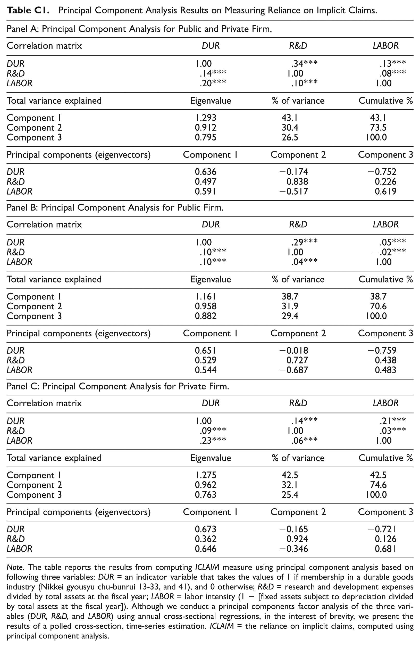
Note. The table reports the results from computing ICLAIM measure using principal component analysis based on following three variables: DUR = an indicator variable that takes the values of 1 if membership in a durable goods industry (Nikkei gyousyu chu-bunrui 13-33, and 41), and 0 otherwise; R&D = research and development expenses divided by total assets at the fiscal year; LABOR = labor intensity (1 − [fixed assets subject to depreciation divided by total assets at the fiscal year]). Although we conduct a principal components factor analysis of the three variables (DUR, R&D, and LABOR) using annual cross-sectional regressions, in the interest of brevity, we present the results of a polled cross-section, time-series estimation. ICLAIM = the reliance on implicit claims, computed using principal component analysis.
Acknowledgements
The authors appreciate the helpful comments and suggestions received from Bharat Sarath (editor), an anonymous reviewer, Shota Otomasa, Takashi Yaekura, Takashi Obinata, Masaki Yoneyama, Keiichi Oishi, Mikiharu Noma, and the participants at the Sixth Contemporary Disclosure Research, the participants of the workshops conducted at Tokyo University and Kansai University.
Author’s Note
All errors are the responsibility of the authors.
Declaration of Conflicting Interests
The author(s) declared no potential conflicts of interest with respect to the research, authorship, and/or publication of this article.
Funding
The author(s) disclosed receipt of the following financial support for the research, authorship, and/or publication of this article: Shuto gratefully acknowledges the financial support from the Grant-in-Aid for Scientific Research (22730354) from the Ministry of Education, Culture, Sports, Science and Technology of Japan. Iwasaki also acknowledges the financial support from the Grant-in-Aid for Scientific Research (#25780299) from the Ministry of Education, Culture, Sports, Science and Technology of Japan.