Labor Differentiation and Agglomeration in General Equilibrium

Abstract

The aim of this article is to explore the structure of cities as a function of labor differentiation, gains to trade, a fixed cost for constructing the transportation network, a variable cost of commodity transport, and the commuting costs of consumers. Firms use different types of labor to produce different outputs. Locations of all agents are endogenous as are prices and quantities. This is among the first articles to apply smooth economy techniques to urban economics. Existence of equilibrium and its determinacy properties depend crucially on the relative numbers of outputs, types of labor, and firms. More differentiated labor implies more equilibria. We provide tight lower bounds on labor differentiation for existence of equilibrium. If these sufficient conditions are satisfied, then generically there is a continuum of equilibria for given parameter values. Finally, an equilibrium allocation is not necessarily Pareto optimal in this model.

Keywords

city structure heterogeneous labor transportation network general equilibrium.

Introduction

This work will attempt to address some of the classic, but relatively unexplored, questions raised in urban economics that deal with the economics of cities. Our questions include the following. Why do cities form where they do? What are the driving forces behind the formation of cities? What roles do increasing returns, gains to trade, and the location of marketplaces play? What role does the location of firms play? Is market failure necessary for agglomeration? Is perfect competition consistent with spatial modeling? Why do some cities grow faster than others? This set of questions frames our line of research. The answers to these questions have important policy implications, since the predictability of the effects of government actions rests on an understanding of the mechanisms driving the urban economy. The ability of policy makers to make informed decisions about contemporary issues such as government policy pertaining to migration to and from cities, or social policy directed at revitalizing cities, relies on information provided by urban economic theory.

In order to have a theory explaining city formation and structure, it is necessary to construct a class of models in which the locations of all agents are endogenous, including both consumers and firms. As explained in Berliant and ten Raa (1994), the nature of most of the existing literature is partial rather than general equilibrium in the sense that either the locations of consumers or firms are fixed. The literature reviewed here is distinct since the locations of all agents are endogenous, and thus these models have the potential to answer the questions we have posed.

There are many approaches to answering the questions addressed by our model that generally suggest different economic causes for city formation and growth and consequently different modeling strategies. Each theory relies on different forces to explain agglomeration and therefore has different consequences in terms of welfare. So it is important to generate testable hypotheses to distinguish among the theories. We categorize the literature on city formation into four groups, using the Spatial Impossibility Theorem of Starrett (1978), as interpreted in Fujita (1986) and Fujita and Thisse (2002), which states that there is no spatial equilibrium with agglomeration if the following conditions are met: (i) no relocation cost, (ii) consumers’ preferences and firms’ technologies are independent of location, (iii) the economy is closed, (iv) each location has complete competitive markets. Each of the four groups explains agglomeration by relaxing at least one of the hypotheses of the Starrett Theorem.

In the first group, city formation is explained using increasing returns to scale. This group violates (iv) since it assumes imperfect competition. Indeed, Fujita and Krugman (1995, 2000), Fujita, Krugman and Venables (1999), and Krugman (1991, 1993a, 1993b) use a Dixit-Stiglitz framework and increasing returns to generate city formation in a monopolistic competition context.¹ This work was preceded by Fujita (1988), Abdel-Rahman (1988, 1990), and Abdel-Rahman and Fujita (1990).

The second group of models uses spatial externalities to explain city formation (Beckmann 1977; Fujita and Ogawa 1982; Papageorgiou and Smith 1983; ten Raa 1984). These models violate (ii), (iv), or both, since agent utilities or production functions depend on the locations of the other agents and these externalities are not priced.

In the third group, agglomeration is explained by strategic interactions between firms (spatial competition a la Hotelling; for surveys see Gabszewicz and Thisse 1986, 1992). This group also violates (iv) since it assumes imperfect competition.

The fourth group of models (Berliant and Konishi 2000; Berliant and Wang 1993; Wang 1990) uses gains to trade and setup costs of marketplaces and transportation networks to generate agglomeration. This group violates (ii) and (iv), since there may be no marketplace (and consequently no market) at some locations, and therefore agents care about location.

Another explanation for city formation is the differentiation of labor. For example, Rochester, NY, has a highly specialized labor force that serves companies such as Kodak, Xerox, and Bausch and Lomb. These companies employ workers who know about optics and engineering. Another example is Silicon Valley that has a concentration of labor specialized in the production of semiconductors. This idea has not been modeled formally, although some attempts have been made to model the worker choice of human capital investment using very crude spatial structures (Baumgardner 1988; Benabou 1993; Kim 1991). Zenou (2009) surveys this literature and studies labor markets in various imperfect competition or search contexts.

The specific question we address in the present article is How does labor differentiation affect city structure?

In our approach (which can be considered as a fifth group), the formation of cities is explained by labor differentiation, gains to trade, a fixed cost for the transportation network, a variable cost of commodity transport, and the commuting costs of consumers. Since firms are used as marketplaces, our model violates (ii) and (iv) of the Starrett Theorem, similar to the fourth group above.

Observe that in all models of general equilibrium with endogenous locations (including ours), the main problem is to show the existence of a spatial equilibrium and to find its determinacy properties. Why is this a problem? When one introduces space in a general equilibrium framework with a continuum of consumers (and locations) and a finite number of firms, there are nonconvexities for both consumers (the consumption set and preferences are nonconvex due to the discrete choice of one location of residence) and firms (firm reaction correspondences are not convex valued since at given prices, a firm’s profit could be maximized at two different locations), and therefore the usual fixed point theorems relevant for proving existence of an equilibrium do not work.

On the consumer side, we can easily convexify the aggregate demand correspondence with a large number of individuals (see Hildenbrand 1974). Schweizer, Varaiya and Hartwick (1976), Ellickson (1979), and Grimaud and Laffont (1989) have used this technique to prove the existence of a spatial equilibrium. Observe that the number of locations in all of this work is finite. In contrast, our model and the standard models of location theory use a continuum of locations. In this case, Hildenbrand’s type of argument does not necessarily apply. As is common in the literature (see Fujita 1989), we use the bid-rent approach, imposing the condition that consumers can choose only one location, to solve the nonconvexity problem; this technique does not require a fixed point argument or convexity but relies on direct calculations.

How can we solve the firm’s nonconvexity problem? To the best of our knowledge, there are two techniques that work. Both of them fix producer locations, and solutions are computed for nonlocation variables given these locations. The two techniques use different methods of fixing producer locations. The first uses Negishi’s (1960) method that fixes firms at the Pareto optimal locations and more generally fixes the allocation at the Pareto optimum. Then one has to decentralize and find a price system that supports the optimum (see Wang 1990; Berliant and Wang 1993). Obviously, this method does not work if there is a market failure. The second technique consists of characterizing the spatial equilibrium. However, since there is in general a lot of endogenous variables (prices and quantities as usual, but also locations of producers and consumers), the characterization of equilibrium is difficult. This method was used by Fujita and Krugman (1995, 2000) and in order to characterize the equilibrium they resort to specific functional forms (e.g., constant elasticity of substitution [CES] utility functions and a Samuelsonian “iceberg” transport technology). This approach suffers from a lack of robustness in the specification of functional forms as well as from a large indeterminacy in the number and qualitative properties of equilibrium. They select one equilibrium. Moreover, consumer commuting is not allowed by this type of model. In our approach, we also use the (second) technique of calculating the equilibrium directly, but we avoid the problems encountered by Fujita and Krugman (1995, 2000). In essence, due to the interaction of firms, considered to be marketplaces as well for exchanging goods, we are able to characterize their equilibrium locations in general, and therefore to prove existence of equilibrium by employing a fixed point argument for all of the nonlocational variables.

A natural question that comes to mind is why, in a model of general equilibrium with endogenous locations (such as ours), does one not use randomized strategies to alleviate the nonconvexity problem and to prove existence of an equilibrium? Basically, there are two reasons not to use mixed strategies. First, if one studies what happens after a randomization is realized, one can easily end up at an infeasible allocation. For example, each firm randomizes over all possible parcels ex ante, but ex post, firms might happen to pile up on one interval, an ex post infeasible allocation. Mixed strategies also involve precommitment of firms to the parcels they get after randomization, and when the random draw is realized, they might have more profits with a different strategy. The latter effect is common to games allowing mixed strategies. The second, and perhaps more important reason, is that the obvious equilibrium with mixed strategies is where everyone is spread out uniformly by randomizing over all locations: it is the Starrett theorem in the context of randomization. Such an allocation clearly minimizes transport costs. There is no agglomeration, and it is uninteresting just as in the standard Starrett theorem. Equilibrium is an artifact of randomization. This is very similar to what is proposed in Koopmans and Beckmann (1957) as the solution where there is no equilibrium in their quadratic assignment model, and should be rejected for the same reasons.

To be more precise, our model uses a very general setting, allowing a multidimensional location space and multiple firms using different types of labor to produce different output commodities. Locations of all agents are endogenous as are prices and quantities. Firms anticipate the relocation of consumers, but influence land prices through their location decisions. As we shall explain shortly, we stick as close to perfect competition as possible while retaining existence of equilibrium. Firms use compact, convex sets of land while consumers buy densities of land. It is assumed that each firm can use only one type of labor and produce only one type of output. With reference to the labor economics literature, labor differentiation can be viewed either as general or specific human capital depending on the number of firms using a particular type of labor. Within this framework, we characterize the spatial configuration of firms in equilibrium. Firms are adjacent to each other at any equilibrium allocation. This is very similar to the principle of minimum differentiation although the force that is driving agglomeration in our model is the transportation cost of outputs. This result is used to prove existence and to examine the determinacy of equilibrium. The proof of existence is unusual in that it uses a mixture of bid rent and fixed point techniques. Concerning the determinacy analysis, we use differential topology techniques in combination with the bid-rent approach. This article can be counted among the first applications of smooth economy techniques to urban economics. To our knowledge, Berliant and Kung (2006, 2009) are the only predecessors, and they apply these techniques to New Economic Geography models.

We show that whether or not equilibrium exists and whether or not it is locally unique depends crucially on the relative numbers of outputs, types of labor, and firms. The multiplicity of equilibria is positively associated with the degree of labor differentiation. Finally, an equilibrium is not necessarily Pareto optimal in this model.

Loosely speaking, our main conclusion is as follows. When labor is not completely differentiated, in the sense that more than one firm is drawing from the same pool of labor, equilibrium might not exist; a counterexample (example 4) is provided in the Online Appendix. (This does not exclude existence of equilibrium for other examples.) Once one has sufficient conditions on labor differentiation for existence of equilibrium, generically there is a continuum of equilibria. This derives from the classical idea that indivisibilities, particularly in the order and location of firms in our model, both inhibits existence of equilibrium and, once equilibrium is found, allows variation in continuous endogenous parameters without altering the order of firms and without destroying equilibrium.

The remainder of the article is organized as follows. The second section sets up the model and provides the notation and basic definitions. In the third section, we characterize the locations of firms and consumers in equilibrium. It is unusual to be able to do this analytically. The fourth section examines the determinacy of equilibrium in this model. For given values of the exogenous parameters, we find that, depending on the number of labor types, firms, and output goods, the set of equilibria might be empty, might be finite, or might form a continuum. The fifth section provides sufficient conditions for existence of an equilibrium in the model. These conditions, in turn, imply that generically the set of equilibria forms a continuum. In the sixth section, we give an example showing that both welfare theorems can fail. The seventh section concludes. An Online Appendix, available at the first author’s website, contains complementary illustrative examples and all proofs.

The General Setting

The location space $Z$ is a compact, convex subset of the Euclidean space $ℜ^{K}$ .² Land of density $1$ is available in all locations in $Z$ . There are $V$ types of labor, $v = 1, . . ., V$ . Each consumer is classified into one category of labor. This could, for example, be derived from the endogenous choice of human capital by consumers as in Rosen (1983), Kim (1989), or Baumgardner (1988). However, here we assume that labor heterogeneity is exogenous. There are $s = 1, . . ., S$ goods and each firm produces only one type of good $s$ . Each worker of a given type has the same utility function and is endowed with one unit of labor but no consumption commodities. $N^{v}$ is the measure of consumers who supply labor of type $v$ . Each individual³ of type $v$ chooses location $z \in Z$ , land consumption $q^{v} (z)$ (where $q (z) = [q^{1} (z), . . ., q^{V} (z)]$ ), and consumption good quantities $X_{s}^{v} (z)$ in order to maximize utility $U^{v} (q^{v} (z), X^{v} (z))$ , where $X^{v} (z)$ is the vector $[X_{1}^{v} (z), . . ., X_{S}^{v} (z)]$ and $X (z) = [X^{1} (z), . . ., X^{V} (z)]$ , under a budget constraint that will be given later. The consumption set of each consumer is the positive orthant of $ℜ^{S + 1}$ . We assume that utility is strictly monotonic in all arguments and represents $C^{r}$ differentiably strictly convex preferences (see Mas-Colell 1985, chap. 2.6). We also assume that for any $q > 0$ , $X > 0$ , $U^{v} (q, X) > 0 = U^{v} (0, X) = U^{v} (q, 0) = U^{v} (0, 0)$ , so any consumption $(q, X)$ with $q$ and $X$ strictly positive yields higher utility than any consumption on the boundary of $ℜ_{+}^{S + 1}$ . For simplicity, there is no disutility from labor.

Each firm uses only one type of labor, along with land, to produce exactly one output commodity. For each $s = 1, . . ., S$ and $v = 1, . . ., V$ , there are $M_{s}^{v}$ firms producing type $s$ commodity with type $v$ labor, where $L_{s}^{i, v}$ , $Q_{s}^{i, v}$ , and $Y_{s}^{i, v}$ are, respectively, the labor, the land input, and the output of firm $i$ producing good $s$ using type $v$ labor. Each firm is thus characterized by a triple $(i, s, v)$ . Here the index $i$ runs from $1$ to $M_{s}^{v}$ . Define the following vectors: $L_{s}^{v} = [L_{s}^{1, v}, . . ., L_{s}^{M_{s}^{v}, v}]$ , $L_{s} = [L_{s}^{1}, . . ., L_{s}^{V}]$ , $L = [L_{1}, . . ., L_{S}]$ , $Q_{s}^{v} = [Q_{s}^{1, v}, . . ., Q_{s}^{M_{s}^{v}, v}]$ , $Q_{s} = [Q_{s}^{1}, . . ., Q_{s}^{V}]$ , $Q = [Q_{1}, . . ., Q_{S}]$ , $Y_{s}^{v} = [Y_{s}^{1, v}, . . ., Y_{s}^{M_{s}^{v}, v}]$ , $Y_{s} = [Y_{s}^{1}, . . ., Y_{s}^{V}]$ , and $Y = [Y_{1}, . . ., Y_{S}]$ . The production function for firm $(i, s, v)$ is given by $f_{s}^{v} (L_{s}^{i, v}, Q_{s}^{i, v}) = Y_{s}^{i, v}$ . Firms using the same type of labor to produce the same commodity are identical. We assume that $f_{s}^{v} (\cdot)$ is $C^{r}$ with strictly positive derivatives on $ℜ_{+ +}^{2}$ , that $D^{2} f_{s}^{v}$ is negative definite, and that $f_{s}^{v} (L_{s}^{i, v}, 0) = 0$ .

Assuming constant returns to scale would not change the basic results but would change supply functions to correspondences, and this would make the differential topology argument used for the determinacy of equilibrium much more difficult.

In our model, absentee landlords are endowed with all of the land and all of the profit shares but consume only produced goods. It is standard in the literature of urban economics to employ absentee landlords to insulate the model from income effects in order to use a bid-rent approach (see e.g., Fujita 1989). Our results are easily generalized to allow consumers to be endowed with land or profit shares.⁴ We can also allow “absentee” shareholders (as distinct from landlords) to have all the profit shares.

We assume that the markets for all goods (including labor) except land are competitive. This assumption of perfectly competitive markets will be made formal in the statements of the consumer and producer optimization problems and is important in order to prove that equilibrium exists. As we will see later, whatever the assumption on the transportation cost of goods, it is this assumption of perfect competition that makes good prices location independent. We will discuss later the assumption that the land market is not competitive.

Consumers of type $v$ purchase a density of land $q^{v} (z)$ , whereas firms will use an area of land. Let $μ$ be Lebesgue measure on measurable subsets of $ℜ^{k}$ . All measure theoretic statements (such as “almost surely” ) are made with respect to this measure. Let $d$ be a metric on $ℜ^{k}$ . For any Lebesgue measurable $A$ and any $ϵ > 0$ , define

\begin{array}{c} B_{ϵ} (A) = {z \in Z | inf_{y \in A} d (y, z) \leq ϵ} a n d \\ g (A, ϵ) = μ (B_{ϵ} (A)) . \end{array}

Firms use Lebesgue measurable subsets of $Z$ as inputs for production. Let $C$ be any collection of Lebesgue measurable subsets of $Z$ satisfying the following conditions:

(a) For each $A \in C$ , there is a $δ > 0$ such that $B_{ϵ} (A) \in C$ $\forall ϵ \in [0, δ)$ and $g (A, \cdot)$ is twice continuously differentiable on $[0, δ)$ .⁵

(b) Fix any $C_{1}^{1, 1}, . . ., C_{S}^{M_{s}^{v}, V} \in C$ . If some firm is using a positive quantity of land, then there exists a (possibly different) firm $(i, s, v)$ with $μ (C_{s}^{i, v}) > 0$ such that for every $δ^{'} > 0$ there is an $A \in C$ , $A \subseteq C_{s}^{i, v}$ almost surely with $μ (C_{s}^{i, v}) - δ^{'} < μ (A) < μ (C_{s}^{i, v})$ and

inf_{\binom{x \in C_{s}^{i, v}}{y \in C_{s^{^{'}}}^{j, v^{^{'}}}}} ∥ x - y ∥= inf_{\binom{x \in A}{y \in C_{s^{^{'}}}^{j, v^{^{'}}}}} ∥ x - y ∥

$f o r s^{'} = 1, . ., S; v^{'} = 1, . . ., V; j = 1, . . ., M_{s}^{v}; \forall (j, s^{'}, v^{'}) \neq (i, s, v)$ .

For instance, if $Z = [0, 1]^{K}$ , the hyper-rectangles of the form $[\underline{θ}, \overline{θ}] \times [0, 1]^{K - 1}$ aligned parallel to the axes in $ℜ^{K}$ used below will satisfy these conditions, as will many other collections. For assumption (b), the firm parcel that contracts is one at the edge of the economy. The idea behind this assumption is that small expansions and contractions of parcels are possible, so calculus can be used. Cantor sets violate this assumption.

If firm $i$ producing good $s$ and using type $v$ labor chooses a $C_{s}^{i, v} \in C$ , then $Q_{s}^{i, v} = μ (C_{s}^{i, v})$ .

It is very important, at this point, to discuss issues related to the shape and proximity of land parcels to each other, especially as they relate to the rest of the literature. As discussed in Berliant (2007), we can sort models of location by what commodity space is used (and also hope to prove universal theorems that are independent of the choice of commodity space). One alternative is to use a general commodity space (such as the space of all Lebesgue measurable sets) and assume both that consumers like nicely shaped parcels and that producers find them more productive, hoping that nicely shaped parcels arise endogenously as equilibrium or optimal outcomes. This is the approach taken in a line of research developed by the first author and coauthors, culminating in Berliant and Dunz (2004). Production in this setting appeared first in Berliant and Jeng (1990), though productivity is not a function of shape in that ancient paper. Key to this literature is a new topology on sets, called the outer Hausdorf topology, which makes the commodity space compact but still allows preference for shape. Convexity/concavity properties are a big hurdle themselves. It is very difficult to characterize equilibrium parcels in this setting outside of some examples. Another alternative, used here as well as in more applied settings such as Berliant and Fujita (1992), is to exogenously restrict the commodity space to allow only nicely shaped parcels. For Theorem 1 below, we use the restriction on land parcels given in (a) and (b) above. But for our most of our results below, we will restrict land parcels even further to hyper-rectangles.

Consumers pay a commuting cost to travel to work. For simplicity, commuting costs are only monetary costs and therefore there is no time cost of commuting. Let $t$ denote the vector of input requirements for one unit of commuting distance, so the cost per unit is $p (i, s, v) \cdot t$ (where $p (i, s, v)$ is the vector of prices of the output goods, $p (i, s, v) \in ℜ_{+}^{s}$ , $t \in ℜ^{s}$ ). Observe that $p (i, s, v)$ is a price vector at a firm-market place so prices are firm (and hence location) dependent. Consumers of type $v$ are employed only by firms using type $v$ labor.

We assume that every pair of firms must be connected by a transport network (the cost of connecting any pair of firms is shared equally by each member of the pair) and that all consumers purchase their consumption goods at the location of a firm, that is firms are marketplaces.⁶ These assumptions mean that transportation of goods takes place only between firms, where consumers purchase all their consumption commodities. The transportation network for commodities will connect all firms, even those producing the same good, since local demand and supply of consumption commodities might not be balanced. For example, this depends on where the absentee landlord shops. The absentee landlord might exhaust the commodity produced by one supplier, requiring that it be imported from another.

In the model, all markets are spatially global, but labor markets can differ due to labor heterogeneity. Variable transport cost can create differences in the price of a consumption good across locations and firms. That is the reason $p (i, s, v)$ is indexed by firm. Later, we shall argue that competition forces $p$ to be constant across firms and hence locations. Observe that the reason that goods must be transported among firms, and the reason that firms must pay a fixed and variable transportation cost, is that consumers use the firms as marketplaces and, due to the boundary condition on preferences, want some of all of the goods.

More formally, let $τ \in ℜ^{s}$ denote the vector of marginal physical requirements for setting up half of a transportation network between two firms, so the cost per unit of distance to firm $(i, s, v)$ is $p (i, s, v) \cdot τ$ . This is a fixed cost independent of volume. Next we specify variable costs.

Let $g_{(j, s^{'}, v^{'})}^{(i, s, v)}$ represent the vector of net shipments of consumption goods between two firms and let $T$ be a nonnegative $S \times S$ matrix. Row $s$ of the matrix $T$ gives the cost in terms of the $S$ consumption goods (per unit of distance) of shipping one unit of consumption good $s$ to or from a firm. A diagonal nonnegative matrix with entries less than 1 would be a Samuelsonian iceberg transport technology.

Our assumption about the cost sharing rule means that this rule is essentially equal division of the network transportation cost for connecting each firm to another. However, our results can be extended to arbitrary monotonic and lower semicontinuous functions of this fixed cost. Relocation costs for both firms and consumers are zero.

We could employ a more general transportation technology as in Berliant and Konishi (2000), which would specify a set of input requirements, each element of which can produce one unit of transportation services. For simplicity, we use the special case given above. The use of a more general technology will not affect the main results, as we shall explain in the third section below. Let us now define two important concepts.

Definition 1: Firm $(i, s, v)$ and firm $(j, s^{'}, v^{'})$ are adjacent if

inf_{\binom{x \in C_{s}^{i, v}}{y \in C_{s^{^{'}}}^{j, v^{^{'}}}}} ∥ x - y ∥ = 0.

Definition 2: Firm $(i, s, v)$ and firm $(j, s^{'}, v^{'})$ are connected if there is a list of firms such that firm $i$ is the first on the list and firm $j$ is the last on the list and each firm is adjacent to its predecessor and successor on the list.

We assume no transport cost between adjacent firms. This implies no transport costs between connected firms, because otherwise firms would simply ship to adjacent firms, and those firms would re-ship to the next firm. Thus, zero transport costs between adjacent firms actually implies zero transport costs among connected firms. Hence, we state the total cost for firm $(i, s, v)$ of a transportation network between firms as follows:

\underset{s^{'} = 1}{\sum^{S}} \underset{v^{'} = 1}{\sum^{V}} \underset{j = 1}{\sum^{M_{s^{^{'}}}^{v^{'}}}} p (i, s, v) \cdot [τ + T \cdot g_{(j, s^{'}, v^{'})}^{(i, s, v)}] inf_{\binom{x \in C_{s}^{i, v}}{y \in C_{s^{'}}^{j, v^{'}}}} ∥x - y∥ \cdot I_{X_{(j, s^{'}, v^{'})}^{(i, s, v)}}

where $I_{X}$ is the indicator function of the event $X$ and $X_{(j, s^{'}, v^{'})}^{(i, s, v)}$ = {Firm $(i, s, v)$ is not connected to firm $(j, s^{'}, v^{'})$ }. Notice that we separate the last two parts of this expression, since firms that are connected are not necessarily adjacent. Observe that even when firms are connected, commuting distance and thus commuting cost of a worker to various firms is not the same.

Let $\overline{Ψ}$ be the constant (over location) unit price of land to firms. The idea that this must be constant will be explained after the statement of the firm’s optimization problem. Firm $(i, s, v)$ maximizes its profit $π_{s}^{v}$ (firms using the same input $v$ and output $s$ are identical) by solving the following problem, taking as given the locations of other firms. To give meaning to other firms’ choices, let $C_{s}^{- (i, s, v)} = [C_{1}^{1, 1}, . . ., C_{s}^{i - 1, v}, C_{s}^{i + 1, v}, . . ., C_{S}^{M_{S}^{V}, V}] .$ $C_{s}^{i, v} \in C$ represents the choice of parcel. For now, we take good shipments $g_{(j, s^{'}, v^{'})}^{(i, s, v)}$ to be exogenous, but shortly we shall see that $T$ can be taken to be zero without loss of generality, so $g_{(j, s^{'}, v^{'})}^{(i, s, v)}$ is immaterial.

max_{L_{s}^{i, v}, C_{s}^{i, v}} π_{s}^{v} (L_{s}^{i, v}, C_{s}^{i, v}, C_{s}^{- (i, s, v)})

where

\begin{aligned} π_{s}^{v} (L_{s}^{i, v}, C_{s}^{i, v}, C_{s}^{- (i, s, v)}) & = p_{s} (i, s, v) f_{s}^{v} (L_{s}^{i, v}, μ (C_{s}^{i, v})) - w^{v} L_{s}^{i, v} - μ (C_{s}^{i, v}) \overline{Ψ} \\ - \underset{s^{'} = 1}{\sum^{S}} \underset{v^{'} = 1}{\sum^{V}} \underset{j = 1}{\sum^{M_{s^{^{'}}}^{v^{^{'}}}}} p (i, s, v) \cdot [τ + T \cdot g_{(j, s^{'}, v^{'})}^{(i, s, v)}] inf_{\binom{x \in C_{s}^{i, v}}{y \in C_{s^{'}}^{j, v^{'}}}} ∥x - y∥ \cdot I_{X_{(j, s^{'}, v^{'})}^{(i, s, v)}} . \end{aligned}

Notice that a firm does not think that changing its location will affect its unit price of land $\overline{Ψ}$ or any other price.

Observe that the profit function depends on the location of firm $(i, s, v)$ and the locations of all other firms through the fourth term of the RHS of equation (1). This is the Nash assumption about equilibrium. When a firm moves, it takes as given the locations of other firms. Here, in terms of location, consumers are behaving competitively whereas firm behavior is Nash. The concept of equilibrium we have here is a sort of a combination of the ones introduced by Fujita and Thisse (1986) and Anderson and Engers (1994). Indeed, in the first paper a land market is considered in the Hotelling model and the authors introduce the possibility of workers’ relocation in reaction to firms’ location decisions. Thus, consumers are the followers in a Stackelberg game where firms are the leaders. In the second paper, firms are price taking but have Nash behavior in location; consumer locations are fixed. It is important to highlight here that our concept of equilibrium is Nash in location but firms take all prices (good prices as well as wages) as given. In other words, each firm moves, taking prices and the location of other firms as given.

Observe moreover that, when a firm changes its location and locates farther away from other firms, this firm might think that its variable transportation cost will go up but, since it is competitive (in the product market), it thinks its output price would not change. Therefore, even with the assumption of positive variable transportation costs, good prices are not location dependent.

This implies location-independent (good and labor) prices. Thus, we have a constant wage gradient, which is just a special case of allowing wages to vary across locations. If wages are allowed to vary across firm locations but agents take the wage gradient as parametric, we would simply have more equilibria. Notice that if one type of worker can be used to produce two different products, although the equilibrium wage rate can be different, in equilibrium the utility of the workers of the same type must be the same. Thus, wage inequality for workers of the same type does not reflect inequality in terms of welfare.

If wages vary with residential distance from a firm, this is a form of price discrimination and seems to be incompatible with perfect competition. In this case, it is unclear what firms think wages would be if they move. Moreover, it seems unrealistic to assume that firms wage discriminate based on the residence locations of worker/consumers.

There are several alternative equilibrium concepts that could be used with this model. We use the simplest, namely perfect competition, taking prices and the actions of other agents as given, with one small deviation. We assume that the price of land faced by firms is constant across locations. An implication is that it is independent of consumer bid rent or the unit price of land paid by consumers. Another implication is that, in equilibrium, the price of land faced by firms will be at least as high as the maximal bid rent of consumers.

There are two reasons we make this assumption. First, the firms know that if they relocate, consumers will follow and bid up the price of land nearby. Although it would be best to model this process explicitly, the resulting model would be very complex and difficult to analyze. In particular, nonconvexities in reaction correspondences of firms would make the analysis attempted here impossible. Instead, we model this process implicitly through a constant price of land for firms.

Second, it is clear that at any possible equilibrium allocation, the bid-rent curves of consumers are highest near a firm and decline with distance from a firm. If firms pay the price given by the highest bid rent for parcels and have location-independent production functions, they will always want to locate where rent is lowest, namely as far away from their current location as possible. Such behavior is unlikely to lead to an equilibrium.

Perhaps the most natural alternative equilibrium concept is as follows. There are two stages, and the solution concept is pure strategy subgame perfect Nash equilibrium. The second stage is an equilibrium under perfect competition given fixed firm parcels. The first stage is a simultaneous move Nash equilibrium with firms choosing the parcels that they will use in production and will rent in the second stage. The firms know perfectly how their choice of parcel in the first stage will affect equilibrium in the second stage, including their land rent and the value of their output.

Although this equilibrium concept has intuitive appeal, there are three serious technical problems associated with it. First, the second stage competitive equilibrium will not be unique in general. This presents problems for both results concerning existence of equilibrium and determinacy of equilibrium. Of course, multiple equilibria in the second stage can cause nonconvexities in (or an ill-defined) first stage reaction correspondence. Possible remedies include using mixed strategies in the first stage, refining second stage equilibria so that they are unique, or imposing conditions on the economy so that second stage equilibria are unique. Any of these solutions will either complicate matters or limit the robustness of results substantially.

The second technical problem is that firms might not be connected in an equilibrium. Prices of mobile goods in the second stage can differ across locations, rendering the equilibrium concept very complex. Nonconvexities in first stage firm reaction correspondences can result. Moreover, the arguments we use for existence of an equilibrium and determinacy properties would no longer work, since they take as given the locations of firms.

The third technical problem with the alternative equilibrium concept is that if firms in the first stage choose a disequilibrium configuration, for example if two firms decide to use the same parcel of land, then payoffs are not well defined. The reason is that given such firm location choices, the second stage configuration of firms is not feasible, so there is no competitive equilibrium associated with it.

For these reasons, we use the first equilibrium concept, employing (virtually) perfect competition. This can be seen as a special case of the alternative equilibrium concept, where the transport cost faced by firms is much larger than the commuting cost faced by consumers, so that firms will always choose to form a connected set in equilibrium.

Let us turn to the consumer’s problem. A consumer of type $v$ performs the following optimization program taking as given prices, $p = [p_{1}, . . ., p_{S}]$ , the wage rate, $w^{v}$ , the integrable land rent, $Ψ : Z \to ℜ_{+}$ , and the location of all firms where $C_{s}^{v} = [C_{s}^{1, v}, . . ., C_{s}^{M_{s}^{v}, v}]$ , $C_{s} = [C_{s}^{1}, . . ., C_{s}^{V}]$ , $C^{v} = [C_{1}^{v}, . . ., C_{S}^{v}]$ , and $C = [C_{1}, . . ., C_{S}]$ .

max_{X^{v}, q^{v}, z} U^{v} (q^{v}, X^{v}) s . t . p \cdot X^{v} + q^{v} Ψ (z) + p \cdot t inf_{\underset{\underset{s = 1, . . ., S}{i = 1, . . ., M_{s}^{v}}}{y \in C_{s}^{i, v}}} ∥z - y∥ = w^{v}

Observe that there is only one wage for each labor type since consumers are mobile and one unit of labor is supplied inelastically by each consumer. Define $w = [w^{1}, . . ., w^{V}]$ .

Let us denote by $R_{s}^{i, v} = {z \in Z | (i, s) \in \underset{\underset{s^{'} = 1, . . ., S}{i^{'} = 1, . . ., M_{s}^{v}}}{arg min} (inf_{y \in C_{s^{'}}^{i^{'}, v}} ∥z - y∥)}$ , the set of locations from which firm $(i, s, v)$ draws its labor.

Let us now consider the absentee landlord’s problem. Let $X^{L} = [X_{1}^{L}, . . ., X_{S}^{L}]$ , $π^{v} = [π_{1}^{v}, . . ., π_{S}^{v}]$ and $π = [π^{1}, . . ., π^{V}]$ . So, the absentee landlord utility function is $U^{L} (X^{L})$ , and we assume that it has the same standard properties as the consumer utility function. The absentee landlord program is therefore:

max_{X^{L}} U^{L} (X^{L}) s . t . p \cdot X^{L} = \int_{Z} Ψ (z) d z + \underset{s = 1}{\sum^{S}} \underset{v = 1}{\sum^{V}} M_{s}^{v} π_{s}^{v}

where $X^{L} (\int_{Z} Ψ (r) d r, π)$ is the “argmax” of equation (3).

The following are standard definitions.

If D is a Lebesgue measurable subset of $Z$ , then $1_{D}$ is the indicator function of the set $D$ , namely $1_{D} (x) = 1$ if $x \in D$ and $1_{D} (x) = 0$ otherwise. Let $n^{v} (z)$ be the density of population of type $v$ at location $z$ , with $n = [n^{1}, . . ., n^{V}]$ . For the matrix T and the vector $g$ , let $T \cdot g = [(T \cdot g)_{1}, . . ., (T \cdot g)_{S}]$ .

Definition 3: A feasible allocation is a vector $(C, L, X (\cdot), q (\cdot), Y, X^{L}, n (\cdot))$ such that $\forall i, s, v,$ $C_{s}^{i, v} \in C$ , $L_{s}^{i, v} \geq 0$ , $Y_{s}^{i, v} \geq 0$ ; $X^{L} \in ℜ_{+}^{S}$ ; and $X : Z \to ℜ_{+}^{S}$ , $q : Z \to ℜ_{+}$ and $n : Z \to ℜ_{+}^{V}$ are measurable functions, such that:

\underset{s = 1}{\sum^{S}} \underset{v = 1}{\sum^{V}} \underset{i = 1}{\sum^{M_{s}^{v}}} 1_{C_{s}^{i, v}} (z) + \underset{v = 1}{\sum^{V}} n^{v} (z) q^{v} (z) = 1 a l m o s t s u r e l y f o r z \in Z

\int_{Z} n^{v} (z) d z = N^{v} v = 1, . . ., V

L_{s}^{i, v} = \int_{R_{s}^{i, v}} n^{v} (z) d z s = 1, . . ., S, v = 1, . . ., V, i = 1, . . ., M_{s}^{v}

Y_{s}^{i, v} = f_{s}^{v} (L_{s}^{i, v}, μ (C_{s}^{i, v})) s = 1, . . ., S, v = 1, . . ., V, i = 1, . . ., M_{s}^{v}

\underset{s = 1}{\sum^{S}} \underset{s^{^{'}} = 1}{\sum^{S}} \underset{v = 1}{\sum^{V}} \underset{v^{^{'}} = 1}{\sum^{V}} \underset{i = 1}{\sum^{M_{s}^{v}}} \underset{j = 1}{\sum^{M_{s^{^{'}}}^{v^{^{'}}}}} [τ_{s} + (T \cdot g)_{s}] inf_{\binom{x \in C_{s}^{i, v}}{y \in C_{s^{^{'}}}^{j, v^{^{'}}}}} ∥x - y∥ \cdot I_{X_{(j, s^{^{'}}, v^{^{'}})}^{(i, s, v)}}

+ \int_{Z} X_{s}^{v} (z) n^{v} (z) d z + X_{s}^{L} + \underset{v = 1}{\sum^{V}} \int_{Z} n^{v} (z) t_{s} \underset{\underset{\underset{s = 1, . . ., S}{i = 1, . . ., M_{s}^{v}}}{y \in C_{s}^{i, v}}}{(inf} ∥z - y∥) d z = \underset{v = 1}{\sum^{V}} \underset{i = 1}{\sum^{M_{s}^{v}}} Y_{s}^{i, v} s = 1, . . ., S

Equation (4) is the material balance condition for land. Notice that one unit of land is available at each point in $Z$ and all land is used. This is due to the fact that we have assumed that both preferences and production functions are monotonic, which implies that land is productive. In one dimension, this is a linear city. Our model can easily be generalized to an arbitrary supply density for land. Equation (5) is the population balance condition. Equation (6) is the material balance condition for local labor markets.⁷ Equation (7) is production feasibility and equation (8) is material balance for the product markets. At a feasible allocation, firm $(i, s, v)$ is (almost surely) the only employer of workers in $R_{s}^{i, v}$ .

Definition 4: An equilibrium is a vector

(p^{*}, {\overline{Ψ}}^{*}, Ψ^{*} (\cdot), w^{*}, C^{*}, L^{*}, X^{*} (\cdot), q^{*} (\cdot), Y^{*}, X^{L^{*}}, n^{*} (\cdot))

such that $(C^{*}, L^{*}, X^{*} (\cdot), q^{*} (\cdot), Y^{*}, X^{L^{*}}, n^{*} (\cdot))$ is a feasible allocation, $p^{*} \in ℜ_{+}^{S}$ , ${\overline{Ψ}}^{*} \in ℜ_{+}$ , $Ψ^{*} : Z \to ℜ_{+}$ is measurable, $w^{*} \in$ $ℜ_{+}^{V}$ , $Ψ^{*} (z) = {\overline{Ψ}}^{*}$ almost surely for $z \in \underset{s = 1}{\overset{S}{\cup}} \underset{v = 1}{\overset{V}{\cup}} \underset{i = 1}{\overset{M_{s}^{v}}{\cup}} C_{s}^{i, v *}$ , and such that, for each $s$ , for each $v$ , for each $i$ , $L_{s}^{i, v^{*}}$ and $C_{s}^{i, v^{*}}$ solve equation (1), and such that, for each $v$ , and almost every $z \in Z$ , $X^{v^{*}} (z)$ and $q^{v^{*}} (z)$ solve equation (2), and finally such that $X^{L^{*}}$ solves equation (3).

Definition 5: An equal treatment Pareto optimum is a feasible allocation

(C, L, X (\cdot), q (\cdot), Y, X^{L}, n (\cdot))

such that for each $v$ , for each $z$ and $z^{'}$ with $n^{v} (z) > 0$ and $n^{v} (z^{'}) > 0,$ $u^{v} = U^{v} (q^{v} (z), X^{v} (z)) = U^{v} (q^{v} (z^{'}), X^{v} (z^{'})),$ and such that there is no feasible allocation $(C^{'}, L^{'}, X^{'} (\cdot), q^{'} (\cdot), Y^{'}, X^{L^{'}}, n^{'} (\cdot))$ such that $U^{L} (X^{L^{'}}) \geq U^{L} (X^{L})$ and for all $v$ and all $z$ with $n^{v^{'}} (z) > 0,$ $U^{v} (q^{v^{'}} (z), X^{v^{'}} (z)) \geq u^{v}$ , with strict inequality holding for a set of consumers of positive measure or for the absentee landlord.

What does equilibrium look like?

Example 1, found in the Online Appendix, motivates our first result and gives us good intuition about equilibrium in the case of two firms and two types of workers. We state the general result.⁸

Theorem 1: Fix any equilibrium land allocation for firms, $C$ . Then it has the property that all firms using positive Lebesgue measure of land are connected (in the sense of Definition 2).⁹ Thus, without loss of generality, we can take equilibrium interfirm transportation costs to be zero.

The following comments are in order. First, in one dimension ( $K = 1$ , a linear city), the city is monocentric since the firms are connected. However, contrary to the standard urban economics literature (Fujita 1989), the Central Business District (CBD) is not a point but a set of firms interacting with each other. It is in this sense the same kind of result as that obtained by Fujita and Ogawa (1982). In two dimensions ( $K = 2$ , a circular city for example), the city can be monocentric or the firms can form any connected set, including an annulus or rectangle. We can have, for example, a circular city where all firms occupy all the locations on the fringe whereas the consumers reside inside the ring.

Second, since a firm takes everything as given except for transport costs (variable or fixed, or both), it will seek to minimize them. Thus, Theorem 1 will work even with positive variable transportation costs, provided that these costs are zero when two firms are connected. Thus, variable costs can be taken to be zero without loss of generality, since firms will be connected in equilibrium in any case. Now consider the case where variable transportation costs are non-zero even when firms are connected. Positive variable costs make no difference, in equilibrium, where they are absorbed by the producer. In this case, they simply are drawn from profits and can only have the effect of reinforcing the agglomeration of firms. An alternative assumption is that they are passed on to consumers in the form of higher prices for consumption goods. In this case, variable transport costs are irrelevant to a firm’s decision problem, since the firm does not pay them. Once again, Theorem 1 applies and firms are connected in equilibrium due to the fixed set-up cost of the transport network. Of course, intermediate cases, where variable transport costs are partially passed through to consumers via higher prices and partially absorbed by producers, are possible. Theorem 1 is robust to these variations since variable transport costs only serve to reinforce the agglomeration of firms. Variable costs will only drive firms together or, if costs are passed to consumers, be neutral.

Third, the assumption of zero transport costs between connected firms is not necessary to obtain Theorem 1. We simply must assume that total transport costs for a firm are minimized when the firm is connected to every other. For example, we could add a constant to the transport costs between firms, independent of location. If two firms are connected, then the transport cost is just this constant. If the two firms are not connected, then it is the constant plus the cost defined in the second section. This obviously leads to no alteration in the result and proof of Theorem 1. It will also be obvious that results in the fourth, fifth, and sixth sections will still be valid, provided that the constant does not exceed a firm’s profits.

More generally, the result given in Theorem 1 holds when the transportation cost function for a firm is any monotonic increasing function of the pairwise (closest point) distances between the firm in question and every other firm, except that it is assumed that the minimum of the function is attained when all firms are connected. In other words, transportation cost is a function of the entire configuration (specifically, when all firms are connected), not just pairwise distances. This function is lower semicontinuous, but it might not be continuous. The addition of a constant to the cost function given in the second section is a special case of this, as specified just above. The result can be extended even further. For example, consider the case when the location space is two dimensional. Assume that the transportation cost of a firm is equal to a monotonic function of pairwise distances between it and every other firm except in the case when the configuration of firm locations (i.e. the land they use) is convex; in the latter case we assume that the function reaches its minimum (as in the case of connected firms above). Then the same proof gives us that in any equilibrium (if it exists), the configuration of firms is convex. Of course the question of existence is then more difficult, since fewer configurations of firms are possible in equilibrium, so (as we shall see) labor must be more differentiated to give enough freedom in endogenous variables to prove that such an equilibrium exists. What we are saying, in essence, is that the equilibrium configuration is driven by assumptions about the transport costs faced by firms. The assumptions, in turn, are informed by our understanding of real-world cost functions as well as common sense, but variations are certainly compatible with the model and the techniques. Therefore, we can force any configuration of firms we choose as cost minimizing to be a necessary condition for an equilibrium using the ideas above.

Although these alterations would represent a stronger or a different result, we do not view them as substantial. In the end, the result is driven by what we assume to be the configuration that minimizes transport cost for the firms. Why do we not simply assume that in equilibrium, firms are connected? We could do that, but there are two issues. First, this is not an assumption on primitives. Second, for the purpose of welfare analysis in sixth section below, we need to calculate explicitly the cost of pulling firms apart, particularly for allocations that are not equilibria.

Last, at an equilibrium in which all firms are connected, the land price of any firm inside the interval (in one dimension) is constant and at least as large as the bid rents at the boundaries of the two extreme firms. In equilibrium, it is indeed not possible that any firm has a lower land price since the one next to it will be induced to move into the land area of the firm in question if the land price is lower. To see this, consider an “equilibrium” where land prices are not constant across connected firms. If land price is decreasing at the boundary of the land used by a particular firm, and if this firm expands its land use in the direction where the price is decreasing, the firm is not maximizing its profit since the marginal revenue product of land exceeds its cost. Although the first-order conditions for profit maximization of this particular firm might be satisfied at the “equilibrium” allocation, a marginal expansion of the firm land usage will yield greater profit since the second-order conditions for profit maximization will not be satisfied when land price decreases. Therefore, equilibrium land price is constant locally around this boundary of the firm’s land parcel. Moreover, our definition of equilibrium requires that the price of land is constant within a firm’s parcel. In fact, if it relocates it thinks the land price is constant and the same as at its current location.

A consequence of the assumption that firms think their land price is constant is a flat equilibrium rent gradient for all firms. This might be hard to accept, but there is some empirical evidence for it; see Schmenner (1981).

Determinacy of equilibrium

Examples 2 and 3, contained in the Online Appendix, illustrate the determinacy properties of equilibrium. We now study the general case by examining the dimension of the set of equilibria (the equilibrium manifold) for a fixed set of exogenous parameters. First, let us define the bid-rent functions.

The bid-rent approach is a well-known technique in urban economics using duality theory to find the maximal willingness to pay for land at each location (see Fujita 1989). The consumer with maximal willingness to pay at a location will live there in equilibrium. Our innovations are to combine it with differential topology methods for use in determinacy analysis, and to combine it with fixed point methods for use in proving existence of equilibrium. Moreover, we extend bid rent from a one-dimensional to a multidimensional tool.

Let $Z = [0, 1]^{K}$ . Let firm $(i, s, v)$ use the hyper-rectangle $C_{s}^{i, v} \equiv [ω^{h}, ω^{h + 1}] \times [0, 1]^{K - 1}$ where $h = \sum_{s^{'} < s} \sum_{v^{'} < v} M_{s^{'}}^{v^{'}} + i$ . In this way, firms are always connected. Then $Q_{s}^{i, v} \equiv ω^{h + 1} - ω^{h}$ , and let $\overset{ˉ}{ω} = (ω^{[\underset{s = 1}{\sum^{S}} \underset{v = 1}{\sum^{V}} M_{s}^{v}] + 1} + ω^{1}) / 2$ be the midpoint of firm land use.

For this subsection only, we must alter our commuting cost function. The reason is that, as specified, it is not $C^{1}$ at zero distance. Thus, for this subsection, we will take it to be a general $C^{1}$ function $t : ℜ_{+} \to ℜ_{+}^{s}$ that is nondecreasing. For example, $t (\cdot)$ could be quadratic.

Definition 6: The bid-rent function for a type $v$ worker at a given location $z$ is defined to be:

Ξ^{v} (z, p, w^{v}, C^{v}, u^{v}) = max_{X^{v}, q^{v}} {[w^{v} - p \cdot X^{v} - p \cdot t (inf_{\underset{\underset{s = 1, . . ., S}{i = 1, . . ., M_{s}^{v}}}{y \in C_{s}^{i, v}}} ∥z - y∥)] / q^{v} | U^{v} (q^{v}, X^{v}) = u^{v}}

Define $X^{v} (z, p, w^{v}, C^{v}, u^{v})$ and $q^{v} (z, p, w^{v}, C^{v}, u^{v})$ to be the argmax of equation (9). Of course, there might not be a solution to (9).¹⁰ This can happen in several different ways, generally at boundaries. For example, $u^{v}$ might specify a level of utility above the supremum utility in the range of the utility function. In that case, one would want to set $Ξ^{v} = 0$ , $q^{v} = \infty$ and $X^{v} = \infty$ . Another possibility is a negative value for $Ξ^{v}$ , which does not cause problems and is thus permissible. If the prices of some consumption goods are zero, then one would want to set consumption of those goods to infinity, consumption of all other goods (including land) to zero, and bid rent at infinity. Finally, if utility were set at its infimum, then one would want to define all consumption levels to be zero and bid rent to be infinite.

These boundary problems have no effect on determinacy analysis, which is next, but can affect the proof of existence of equilibrium. The reason there is no impact on determinacy analysis is that we will restrict our analysis to interior (nonzero) prices and utility levels. We only prove that the system is smooth on this domain; equilibria must reside in this region, so determinacy analysis can proceed where variables do not hit boundaries. Obviously, to prove that an equilibrium exists, behavior of the system on boundaries matters. However, rather than worry about defining bid rent at all of these boundaries, it is easier simply to define excess demand correspondences directly at these boundaries, and be sure that they are upper-hemicontinuous. We shall do this in the proof of Theorem 4.

Since firms are connected in the spatial arrangement we have postulated, transportation (but not commuting) cost can be neglected. This simplifies matters substantially. The optimization problem (1) of firm $(i, s, v)$ becomes:

max_{L_{s}^{i, v}, Q_{s}^{i, v}} π_{s}^{v} = p_{s} f_{s} (L_{s}^{i, v}, Q_{s}^{i, v}) - w^{v} L_{s}^{i, v} - Q_{s}^{i, v} \overline{Ψ}

where $\overline{Ψ}$ will be the (uniform) price of land for firms. Define $π_{s}^{v} (p_{s}, w^{v}, \overline{Ψ})$ to be the maximum and define $L_{s}^{i, v} (p_{s}, w^{v}, \overline{Ψ})$ and $Q_{s}^{i, v} (p_{s}, w^{v}, \overline{Ψ})$ to be the argmax of equation (10), all of which exist if $w^{v}$ and $\overline{Ψ}$ are positive. Given our assumptions on production, if a solution to equation (10) exists, it is unique. Given $Q_{s}^{i, v} (p_{s}, w^{v}, \overline{Ψ})$ , define $C_{s}^{i, v} (p_{s}, w^{v}, \overline{Ψ})$ to be the hyper-rectangle given above Definition 6.

Of course, as in the case of bid-rent equation (9), there might not be a solution to equation (10) when the price of an input is zero. Once again, these boundary problems have no effect on determinacy analysis, which is next, but can affect the proof of existence of equilibrium. Thus, we shall take up this issue in the proof of Theorem 4.

We begin by restating the set of equations that define equilibrium. The goal, as in Berliant and Kung (2006), is to reduce the number of equations and endogenous variables from a continuum to a finite number. That is why we use bid rent. Substituting demands and supplies into the feasibility conditions (4)–(8) and using equations (9) and (10), we obtain:

\underset{s = 1}{\sum^{S}} \underset{v = 1}{\sum^{V}} \underset{i = 1}{\sum^{M_{s}^{v}}} 1_{C_{s}^{i, v} (p_{s}, w^{v}, \overline{Ψ})} (z) + \underset{v = 1}{\sum^{V}} n^{v} (z) q^{v} (z, p, w^{v}, C^{v}, u^{v}) - 1 = 0

a l m o s t s u r e l y f o r z \in Z

\int_{Z} n^{v} (z) d z - N^{v} = 0 v = 1, . . ., V

L_{s}^{i, v} (p_{s}, w^{v}, Ψ^{*}) - \int_{R_{s}^{i, v}} n^{v} (z) d z = 0 s = 1, . . ., S, v = 1, . . ., V, i = 1, . . ., M_{s}^{v}

Y_{s}^{i, v} = f_{s}^{v} (L_{s}^{i, v} (p_{s}, w^{v}, \overline{Ψ}), μ (C_{s}^{i, v} (p_{s}, w^{v}, \overline{Ψ}))) s = 1, . . ., S, v = 1, . . ., V, i = 1, . . ., M_{s}^{v}

\underset{v = 1}{\sum^{V}} \int_{Z} X_{s}^{v} (z, p, w^{v}, C^{v}, u^{v}) n^{v} (z) d z + X_{s}^{L} (z, p, w^{v}, C^{v}, u^{v})

+ \underset{v = 1}{\sum^{V}} \int_{Z} n^{v} (z) t_{s} \underset{\underset{\underset{s = 1, . . ., S}{i = 1, . . ., M_{s}^{v}}}{y \in C_{s}^{i, v}}}{(inf} ∥z - y∥) d z = \underset{v = 1}{\sum^{V}} \underset{i = 1}{\sum^{M_{s}^{v}}} Y_{s}^{i, v} s = 1, . . ., S

We assume that for fixed output prices, fixed wages, fixed locations of firms, and fixed utility levels, all the consumer bid-rent functions are well behaved in the sense of Fujita (1989, definition 4.1, p. 99) and that each pair of bid-rent functions crosses on a set of measure zero. A related assumption is that bid-rent functions can be ordered by relative steepness (see assumption 4.3, p. 102 in Fujita 1989). Our definition is different from Fujita’s since consumers work in and thus commute to different places while in Fujita they all work in the same place (the CBD). Formally, the assumption is:

\forall v \neq v^{^{'}}, \forall p, w^{v}, w^{v^{'}}, C^{v}, C^{v^{'}}, u^{v}, u^{v^{'}} a l m o s t s u r e l y f o r z \in Z ∖ \underset{s = 1}{\overset{S}{\cup}} \underset{i = 1}{\overset{M_{s}^{v}}{\cup}} C_{s}^{i, v}

\frac{\partial Ξ^{v} (z, p, w^{v}, C^{v}, u^{v})}{\partial z} \neq \frac{\partial Ξ^{v^{'}} (z, p, w^{v^{'}}, C^{v^{'}}, u^{v^{'}})}{\partial z}

We use this assumption in order to be sure that the bid-rent functions of consumers do not coincide on an open set of locations. For if they were to coincide, the bid-rent approach would not lead to a unique distribution of population. In this case, we would have to deal with aggregate demand correspondences instead of functions and both determinacy and equilibrium analysis would be much more complicated, but the results would likely be similar. Our assumption would follow, for instance, if consumers have Cobb-Douglas utilities where different types of workers have different parameters attached to land consumption. We conjecture that our assumption is generic in utilities, though that idea is far removed from the point of this work.

We also want land consumption for workers and firms, composite good consumption, and firm labor demand to be well defined as functions of profit levels, utility levels, wages, and prices. That is the next step, and we will obtain this result in Lemma 1 below.

We reformulate the equilibrium conditions using a bid-rent approach (see e.g., Fujita and Ogawa 1982 or Fujita 1989).

Let $α : Z \times ℜ_{+}^{S} \times ℜ_{+}^{V} \times C^{\underset{s = 1}{\sum^{S}} \underset{v = 1}{\sum^{V}} M_{s}^{v}} \times ℜ^{V} \to ℜ$ be an arbitrary smooth function (we write $α (z, p, w, C, u)$ , where $u = [u^{1}, . . ., u^{V}]$ are utility levels) so that for all $(p, w, C, u)$ , $\partial α (z, p, w, C, u) / \partial z_{1} < 0 \forall$ $z_{1} < \overset{ˉ}{ω}, \partial α (z, p, w, C, u) / \partial z_{1} > 0 \forall z_{1} > \overset{ˉ}{ω},$ and $inf_{z \in Z ∖ \underset{s = 1}{\overset{S}{\cup}} \underset{v = 1}{\overset{V}{\cup}} \underset{i = 1}{\overset{M_{s}^{v}}{\cup}} C_{s}^{i, v}} α (z, p, w, C, u) \geq sup_{z \in \underset{s = 1}{\overset{S}{\cup}} \underset{v = 1}{\overset{V}{\cup}} \underset{i = 1}{\overset{M_{s}^{v}}{\cup}} C_{s}^{i, v}} {max}_{v = 1, . . ., V} [Ξ^{v} (z, p, w^{v}, C^{v}, u^{v})] .$ The purpose of the function $α$ is to stand in for the maximal bid-rent function, since the latter function is not smooth.¹¹ The restriction on the slope of $α$ will ensure that when the price of land paid by the firms, $\overline{Ψ}$ , is too low, there is excess demand for land. If it is too high, there is excess supply. We let $γ \geq 1$ be a variable that will scale $α$ . Once we have some function $α$ satisfying the requirements just above, $γ \cdot α$ will also satisfy these requirements, leading to another degree of indeterminacy.

Let

\begin{aligned} Z^{v} = {z \in Z ∖ \underset{s = 1}{\overset{S}{\cup}} \underset{v = 1}{\overset{V}{\cup}} \underset{i = 1}{\overset{M_{s}^{v}}{\cup}} C_{s}^{i, v} | γ \cdot α (z, p, w, C, u) \geq \overline{Ψ} \\ a n d 0 \leq Ξ^{v} (z, p, w^{v}, C^{v}, u^{v}) = max_{v = 1, . . ., V} [Ξ^{v} (z, p, w^{v}, C^{v}, u^{v})]} \end{aligned}

\begin{aligned} \cup {z \in \underset{s = 1}{\overset{S}{\cup}} \underset{v = 1}{\overset{V}{\cup}} \underset{i = 1}{\overset{M_{s}^{v}}{\cup}} C_{s}^{i, v} | γ \cdot α (z, p, w, C, u) > \overline{Ψ} \\ a n d 0 \leq Ξ^{v} (z, p, w^{v}, C^{v}, u^{v}) = max_{v = 1, . . ., V} [Ξ^{v} (z, p, w^{v}, C^{v}, u^{v})]} \end{aligned}

Since we shall employ Walras’ law in the context of the bid-rent approach, we must define (out of equilibrium) rent collections:

R (p, w, C, u, \overline{Ψ}) \equiv \underset{v = 1}{\sum^{V}} \int_{Z^{v}} Ξ^{v} (z, p, w^{v}, C^{v}, u^{v}) d z + \overline{Ψ} \cdot μ (\underset{s = 1}{\overset{S}{\cup}} \underset{v = 1}{\overset{V}{\cup}} \underset{i = 1}{\overset{M_{s}^{v}}{\cup}} C_{s}^{i, v})

This is consistent with equation (3) in equilibrium.

The remaining equilibrium equations are

\int_{Z^{v}} \frac{1}{q^{v} (z, p, w^{v}, C^{v} (p_{s}, w^{v}, \overline{Ψ}), u^{v})} d z - N^{v} = 0 v = 1, . . ., V

\begin{aligned} L_{s}^{i, v} (p_{s}, w^{v}, \overline{Ψ}) - \int_{R_{s}^{i, v} \cap Z^{v}} \frac{1}{q^{v} (z, p, w^{v}, C^{v} (p_{s}, w^{v}, \overline{Ψ}), u^{v})} d z = 0 \\ s = 1, . . ., S, v = 1, . . ., V, i = 1, . . ., M_{s}^{v} \end{aligned}

\begin{aligned} \underset{v = 1}{\sum^{V}} \int_{Z} \frac{X_{s}^{v} (z, p, w^{v}, C^{v} (p_{s}, w^{v}, \overline{Ψ}), u^{v})}{q^{v} (z, p, w^{v}, C^{v} (p_{s}, w^{v}, \overline{Ψ}), u^{v})} d z + X_{s}^{L} (R, π) \\ + \underset{v = 1}{\sum^{V}} \int_{Z} \frac{1}{q^{v} (z, p, w^{v}, C^{v} (p_{s}, w^{v}, \overline{Ψ}), u^{v})} t_{s} \underset{\underset{\underset{s = 1, . . ., S}{i = 1, . . ., M_{s}^{v}}}{y \in C_{s}^{i, v}}}{(inf} ∥z - y∥) d z \end{aligned}

\begin{aligned} - \underset{v = 1}{\sum^{V}} \underset{i = 1}{\sum^{M_{s}^{v}}} f_{s}^{v} (L_{s}^{i, v} (p_{s}, w^{v}, \overline{Ψ}), μ (C_{s}^{i, v} (p_{s}, w^{v}, \overline{Ψ}))) = 0 s = 1, . . ., S \\ μ (\{z \in \underset{s = 1}{\overset{S}{\cup}} \underset{v = 1}{\overset{V}{\cup}} \underset{i = 1}{\overset{M_{s}^{v}}{\cup}} C_{s}^{i, v} (p_{s}, w^{v}, \overline{Ψ}) | γ \cdot α (z, p, w, C, u) > \overline{Ψ})\}) \\ - μ (\{z \in Z ∖ \underset{s = 1}{\overset{S}{\cup}} \underset{v = 1}{\overset{V}{\cup}} \underset{i = 1}{\overset{M_{s}^{v}}{\cup}} C_{s}^{i, v} (p_{s}, w^{v}, \overline{Ψ})] | γ \cdot α (z, p, w, C, u) < \overline{Ψ})\}) = 0 \end{aligned}

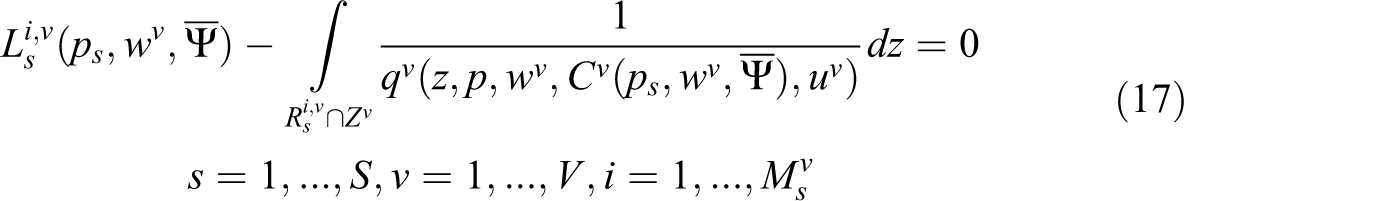
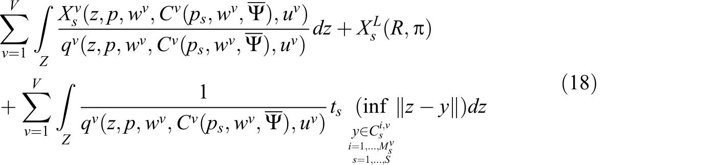
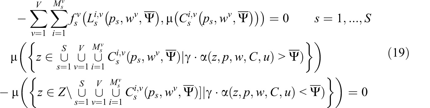
where equation (19) is the market clearing condition for land under the bid-rent approach.

We need to show that the LHS of equations (16) $-$ (19) are continuous functions for the proof of existence and smooth functions for determinacy analysis. Define

Ω^{\circ} = \{(p, w, \overline{Ψ}) | \underset{s = 1}{\sum^{S}} p_{s} + \underset{v = 1}{\sum^{V}} w^{v} + \overline{Ψ} = 1, p_{s} > 0, w^{v} > 0, \overline{Ψ} > 0, s = 1, . . ., S, v = 1, . . ., V\}

and $u^{\circ} = {(u^{1}, . . ., u^{V}) \in ℜ_{+}^{V} | u^{v} > 0$ for $v = 1, . ., V}$ .

We recapitulate our key assumptions here for completeness.

Lemma 1: Suppose that $r \geq 1$ and for each $v$ , $U^{v}$ is $C^{r + 1}$ differentiably strictly convex (and thus has no critical point). Suppose that for each $s$ and $v$ , $f_{s}^{v}$ is $C^{r + 1}$ and that $D^{2} f_{s}^{v}$ is negative definite (thus $f_{s}^{v}$ is strictly concave). Suppose that for each $(z, p, w^{v}, C^{v}, u^{v})$ and $w^{v^{'}}, C^{v^{'}}, u^{v^{'}}$ , $\frac{\partial Ξ^{v} (z, p, w^{v}, C^{v}, u^{v})}{\partial z} \neq \frac{\partial Ξ^{v} (z, p, w^{v^{'}}, C^{v^{'}}, u^{v^{'}})}{\partial z}$ . Suppose that commuting cost as a function of distance to a firm, $t : ℜ_{+} \to ℜ_{+}^{s}$ , is $C^{r}$ with $\frac{\partial t_{s}}{\partial r} \geq 0$ for all $s$ . Finally, restrict attention to those allocations where firms using each type of labor $v$ are connected. Then the equation system (16) $-$ (19) is $C^{r}$ on domain $Ω^{\circ} \times u^{\circ}$ .¹²

To examine determinacy of equilibrium, we use the implicit function theorem (see Mas-Colell 1985, theorem C.3.2, p. 20). If zero is a regular value of the set of functions defined by the LHS of equations (16) $-$ (19), then by the implicit function theorem the set of equilibria forms a manifold of dimension equal to the number of unknowns minus the number of equations. Any regular parameterization (see Mas-Colell 1985, definition 5.8.12, p. 226) of the economies defined by the LHS of equations (16)–(19) will imply that zero is a regular value generically in the parameters; see Mas-Colell (1985, proposition 8.3.1, p. 320). An example of a regular parameterization of our system can be found in our Online Appendix.

This is the point at which the results for models with location, such as this one, begin to diverge from those for more standard models without location. First, notice that there will be a different equilibrium manifold for each order of firms. In essence, the set of all equilibria will be the union of these manifolds. Second, there will be a distinction between the dimension of the equilibrium manifold under symmetry of the configuration of firms as opposed to asymmetry. This latter subject requires a definition.

Definition 7: If for all $v = 1, . . ., V$ and $s = 1, . . ., S$ , except for one $(v^{'}, s^{'})$ , $M_{s}^{v} = 2$ or $M_{s}^{v} = 0$ ,¹³ and either $M_{s^{'}}^{v^{'}} = 1$ or $M_{s^{^{'}}}^{v^{^{'}}} = 0$ , then we call the production sector symmetrizable. An order of firms is a list of all firms by type $(v, s)$ in the economy. An order is called symmetric if it reads the same from left to right as from right to left.

The idea behind this definition is that a production sector is symmetrizable if and only if one can create a symmetric distribution of firms, placing the exceptional firm $(v^{'}, s^{'})$ , if it is present, in the middle of the interval and allocating each pair of identical firms on either side of the exceptional firm so as to create a symmetric distribution. When this is possible, determinacy properties are different.

Theorem 2: Let $K = 1,$ $Z = [0, 1]$ and suppose that the production sector is not symmetrizable. Let $r > min (0, V - \overset{S}{\sum_{s = 1}} \underset{v = 1}{\sum^{V}} M_{s}^{v} + 2)$ .¹⁴ Take any $C^{r}$ regular parameterization of the economies defined by (16)–(19).¹⁵ Fix any order of firms (from left to right). Then generically in parameters, the set of equilibria forms a manifold of dimension:

V - \overset{S}{\sum_{s = 1}} \underset{v = 1}{\sum^{V}} M_{s}^{v} + 2

This theorem is in accordance with examples 2 and 3, found in the Online Appendix. Indeed, in example 3 where $S = 2, V = 2$ and $\overset{S}{\sum_{s = 1}} \underset{v = 1}{\sum^{V}} M_{s}^{v} = 2$ , we obtain two dimensions of indeterminacy, which is consistent with formula (20), generically. Now consider example 2 with $S = 2, V = 1$ and two different firms. It is easy to check by using formula (20) that there is one dimension of indeterminacy (generically).

This means that existence and determinacy of equilibrium are very sensitive to both the degree of labor differentiation and the number of firms. What is the intuition about why the degree of indeterminacy is expressed according to formula (20)? Consider the firms with the same labor input and same output. These firms must have the same profit level in equilibrium. It is the number of such equal profit constraints that affects the formula (20). So as labor becomes more differentiated, there are fewer such constraints. Hence, the more differentiated the labor, the larger the variety of equilibria. Another way of interpreting the intuition behind formula (20) is that identical firms must offer the same wages to the same workers and this cannot compensate for locational and hence commuting cost differences between firms.

Theorem 3: Let $K = 1,$ $Z = [0, 1]$ and suppose that the production sector is symmetrizable. Fix any symmetric order of firms. Let $r > min (0, V - [\overset{S}{\sum_{s = 1}} \underset{v = 1}{\sum^{V}} M_{s}^{v}] / 2 + 1)$ if the number of firms is even, and $r > min (0, V - [\overset{S}{\sum_{s = 1}} \underset{v = 1}{\sum^{V}} M_{s}^{v} + 1] / 2 + 1)$ if the number of firms is odd. Take any $C^{r}$ regular parameterization of the economies defined by (16)–(19). Then generically in parameters, the set of equilibria forms a manifold of dimension:

V - [\overset{S}{\sum_{s = 1}} \underset{v = 1}{\sum^{V}} M_{s}^{v}]/ 2 + 1

if the number of firms is even and

V - [\overset{S}{\sum_{s = 1}} \underset{v = 1}{\sum^{V}} M_{s}^{v} + 1]/ 2 + 1

if the number of firms is odd.

What distinguishes symmetrizable production sectors is that we only need to deal with half (possibly plus one) the number of firms. This means that the number of constraints in a symmetric equilibrium, particularly in equation (17), can be dropped by half (modulo the central firm). The reason the last term in the indeterminacy formula is $1$ for this theorem, whereas it is $2$ for the previous theorem is that under symmetry, $\overset{ˉ}{ω}$ , the midpoint of firm land use, is fixed, whereas under asymmetry, it is not.

In the general case, when $Z$ is not necessarily $[0, 1]$ , the analysis above applies, but it is very difficult to parameterize the location of firms. When $Z = [0, 1]^{K}$ , formula (20) gives only a lower bound on the dimension of the equilibrium manifold, since firms might not be configured in the linear fashion that we have postulated. Configurations that are not rectangular are also possible. At the end of third section, we discussed various configurations of firms. In the most general case, when $Z$ is an arbitrary compact, convex subset of $ℜ^{k}$ , Theorem 1 tells us that firms will be connected but the configuration can vary in a multitude of ways. Hence, it is difficult to draw general conclusions about the determinacy properties of equilibrium when location is multidimensional, except for noting that the general expression for the dimension of the equilibrium manifold becomes larger as labor differentiation increases.

Existence of Equilibrium

Putting aside the problem of multiplicity of equilibria, we next provide sufficient conditions for the set of equilibria to be nonempty. In the Online Appendix, we provide example 4 where formula (22) tells us that equilibria should be locally unique (as the dimension of the equilibrium manifold is equal to zero), but the set of equilibria is in fact empty. This might seem paradoxical given formula (22), but the resolution, of course, is that the empty set is a manifold of any dimension.

Theorem 4: Fix $K$ , a positive integer. Let $Z = [0, 1]^{K}$ . Suppose that labor is completely differentiated, that is $V = \overset{S}{\sum_{s = 1}} \underset{v = 1}{\sum^{V}} M_{s}^{v}$ . Suppose that the assumptions of Lemma 1 hold with $r = 1$ . Then there exists an equilibrium.

We have an analogous result when the production sector is symmetrizable, since in that case only half the firms matter.

Theorem 5: Fix $K$ , a positive integer. Let $Z = [0, 1]^{K}$ . Suppose that the production sector is symmetrizable and that labor is completely differentiated in each half-economy, that is

V = [\sum_{s = 1}^{S} \sum_{v = 1}^{V} M_{s}^{v}]/ 2

if the number of firms is even and

V = [\sum_{s = 1}^{S} \sum_{v = 1}^{V} M_{s}^{v} + 1]/ 2

if the number of firms is odd. Suppose that the assumptions of Lemma 1 hold with $r = 1$ . Then there exists an equilibrium.

In cases not covered by these two theorems, it is easy to generate counterexamples like the one in the Online Appendix. If two firms are drawing their labor supply from the same pool of commuters, one of the firms is going to be farther away from the pool and will never be able to hire the labor it demands at any wage. Example 4 shows that the assumptions on labor differentiation in Theorems 4 and 5 are tight. When these conditions are satisfied, Theorems 2 and 3 imply (generically) that there is a continuum of equilibria.

The method of proof can be extended to more general settings. For instance, $Z$ can be more general. In more general settings, one must be careful with land parcels used by firms since they can hit the boundary of $Z$ ; that is the reason we use the particular connected spatial configuration of firms in this theorem.

Observe also that the assumption that markets for all goods (including labor) except land are competitive is used to prove Theorem 1. Indeed, our equilibrium concept is such that each firm takes all prices as given. If product and labor markets were not competitive, that is firms do not take all prices as given, then firm reaction correspondences would not be convex valued since at given prices, a firm’s profit could be maximized at two different locations. In this case, the existence of equilibrium could not be proved in the way we have done it.

Welfare Properties of Equilibrium Allocations

Theorem 6: An equilibrium allocation might not be Pareto optimal, and in particular might not be an equal treatment Pareto optimum.

The proof (found in the Online Appendix) proceeds by presenting an example where the equilibrium allocation is not Pareto optimal. This is accomplished by taking an equilibrium where the only two firms in the economy are adjacent, pulling them apart a little bit, and putting some consumers in between the firms, thereby reducing commuting costs. Although transportation costs rise, parameters are taken so that this is more than offset by the drop in commuting cost.

Notice that, if a Pareto optimum exists, it will not have adjacent firms (for the reason given in the proof of Theorem 6) and thus will not be an equilibrium allocation. Therefore, the second welfare theorem will also fail for this model and this example, provided that a Pareto optimum exists for this example. We do not prove that a Pareto optimum (equal treatment or otherwise) exists for this example since such a proof is both technical and peripheral to our work here.

Notice also that even though firms and consumers are price takers in all markets, we still have a market failure. More precisely, when a firm moves it anticipates the relocation of its workers, but it does not take into account that it affects workers’ commuting cost and hence utility levels. In a certain sense, there is an externality that causes a market failure.

Conclusion

This article has explained city structure driven by labor differentiation and transportation costs. We have examined the characteristics, welfare properties, existence, and determinacy of equilibrium.

It is immediately apparent from the sixth section that there is a role for the government in improving consumer welfare relative to an equilibrium allocation, since the two welfare theorems can fail. In the one dimensional example, the government might be able to improve welfare by separating firms and reducing consumer commuting cost. It would be interesting to examine this further in a more general setting.

Theorem 1 provides a testable implication of the model: that firms are connected in equilibrium. Comparative static properties of the model are within reach but messy. One can see that the more differentiated the labor, the larger the variety of equilibria. For example, in the homogeneous labor case for $K = 1$ , $V = 1$ , $S = 2$ , supposing that there are $3$ firms producing each of the two products, then there is no equilibrium. When labor is differentiated, $K = 1$ , $V = 6$ , $S = 2$ so that each firm uses a unique type of labor, then generically there is a continuum of equilibria. Thus, the variety of city types is positively related to the degree of labor differentiation, a second testable implication of the model. The collection of essays in Pereira and Mata (1996) provides interesting data on this subject for Portugal.

Our results provide an illustration of the manifestations of indivisibilities in location models. Due to the discreteness with which firms must be ordered in one dimension, the set of equilibria for fixed values of other exogenous parameters can skip from emptiness to a continuum as labor differentiation is increased.

Our model can be extended in the following way. We have taken as exogenous the general and specific human capital of workers. We can make the choice of human capital endogenous by adding a first stage to the model in which each worker chooses an investment in human capital, with perfect foresight, that will determine their skill and type in the second stage. The first stage can be handled in a standard way, for example as in Rosen (1983). The second stage is the model examined in the present article where the populations of the various types of workers are endogenous and determined in the first stage. We intend to examine this more elaborate model in the future.

Finally, a referee has suggested that in place of the relatively simple model we have proposed, multiple types of workers should be introduced into Fujita and Ogawa (1982) and Fujita (1988). Berliant and Kung (2006) examine indeterminacy in a standard New Economic Geography model with one type of mobile worker. That analysis is rather difficult and complex compared to our analysis here, so it is doubtful that definitive statements about the dimension of the equilibrium manifold as a function of labor differentiation can be made. Moreover, Berliant and Kung (2006) find so many equilibria that the predictive capacity of the model is called into question.

Footnotes

Acknowledgments

We thank the anonymous referees, Masahisa Fujita, Roger Guesnerie, Hideo Konishi, Fan-Chin Kung, Val Lambson, Guy Laroque, Thijs ten Raa, Adam Rose, Jacques-François Thisse and Ping Wang, for valuable comments. The first draft of this article was written while the first author was visiting CORE in 1995. The authors retain full responsibility for any errors.

Declaration of Conflicting Interests

The author(s) declared no potential conflicts of interest with respect to the research, authorship, and/or publication of this article.

Funding

The author(s) disclosed receipt of the following financial support for the research, authorship, and/or publication of this article: The authors received financial support from CORE and National Science Foundation grant SBR-9319994.

Notes

References

Abdel-Rahman

1988. “Product Differentiation, Monopolistic Competition and City Size.” Regional Science and Urban Economics 18:69–86.

Abdel-Rahman

1990. “Agglomeration Externalities, Types, and Sizes of Cities.” Journal of Urban Economics 27:25–45.

Abdel-Rahman

Fujita

. 1990. “Product Variety, Marshallian Externalities, and City Sizes.” Journal of Regional Science 30:165–83.

Anderson

Engers

. 1994. “Spatial Competition with Price-Taking Firms.” Economica 61:125–36.

Baumgardner

1988. “The Division of Labor, Local Markets, and Worker Organization.” Journal of Political Economy 96:509–27.

Beckmann

1977. “Spatial Equilibrium: A New Approach to Urban Density.” In Resource Allocation and Division of Space, edited by Fujii and Sato, 121–30. Berlin, Germany: Springer-Verlag.

Benabou

1993. “Workings of a City: Location, Education, and Production.” Quarterly Journal of Economics 108:619–52.

Berliant

2007. “Prospects for a Unified Urban General Equilibrium Theory.” Regional Science and Urban Economics 37:466–71.

Berliant

Dunz

. 2004. “A Foundation of Location Theory: Existence of Equilibrium, The Welfare Theorems and Core.” Journal of Mathematical Economics 40:593–618.

10.

Berliant

Fujita

. 1992. “Alonso’s Discrete Population Model of Land Use: Efficient Allocations and Competitive Equilibria.” International Economic Review 33:535–66.

11.

Berliant

Jeng

H.-W.

. 1990. “Supply and Equilibrium in an Economy with Land and Production.” International Economic Review 31:799–828.

12.

Berliant

Konishi

. 2000. “The Endogenous Formation of a City: Population Agglomeration and Marketplaces in a Location-Specific Production Economy.” Regional Science and Urban Economics 30:289–324.

13.

Berliant

Kung

F.-C.

. 2006. “The Indeterminacy of Equilibrium City Formation Under Monopolistic Competition and Increasing Returns.” Journal of Economic Theory 131:101–33.

14.

Berliant

Kung

F.-C.

. 2009. “Bifurcations in Regional Migration Dynamics.” Regional Science and Urban Economics 39:714–20.

15.

Berliant

ten Raa

. 1994. “Regional Science: The State of the Art.” Regional Science and Urban Economics 24:631–47.

16.

Berliant

Wang

. 1993. “Endogenous Formation of a City without Agglomerative Externalities or Market Imperfections: Marketplaces in a Regional Economy.” Regional Science and Urban Economics 23:121–44.

17.

Ellickson

1979. “Competitive Equilibrium with Local Public Goods.” Journal of Economic Theory 21:46–61.

18.

Fujita

1986. “Urban Land Use Theory.” In Location Theory, edited by Lesourne and Sonnenschein, 73–149. New York, NY: Harwood Academic Publishers.

19.

Fujita

1988. “A Monopolistic Competition Model of Spatial Agglomeration: Differentiated Product Approach.” Regional Science and Urban Economics 18:87–124.

20.

Fujita

1989. Urban Economic Theory. Land Use and City Size. Cambridge: Cambridge University Press.

21.

Fujita

Krugman

. 1995. “When is the Economy Monocentric? von Thünen and Chamberlain Unified.” Regional Science and Urban Economics 25:505–28.

22.

Fujita

Krugman

. 2000. “A Monopolistic Competition Model of Urban Systems and Trade.” In Economics of Cities. Theoretical Perspectives, edited by Thisse

J-F.

Huriot

J.-M.

, 167–216. Cambridge: Cambridge University Press.

23.

Fujita

Krugman

Venables

A. J.

. 1999. The Spatial Economy. Cities, Regions, and International Trade. Cambridge, MA: The M.I.T. Press.

24.

Fujita

Ogawa

. 1982. “Multiple Equilibria and Structural Transition of Non-Monocentric Urban Configurations.” Regional Science and Urban Economics 12:161–96.

25.

Fujita

Thisse

J.-F.

. 1986. “Spatial Competition with a Land Market: Hotelling and von Thünen Unified.” Review of Economic Studies 53:819–41.

26.

Fujita

Thisse

J.-F.

. 2002. Economics of Agglomeration. Cities, Industrial Location, and Regional Growth. Cambridge: Cambridge University Press.

27.

Gabszewicz

J. J.

Thisse

J.-F.

. 1986. “Spatial Competition and the Location of Firms.” In Location Theory, edited by Gabszewicz

J. J.

Thisse

J-F.

Fujita

Schweizer

, 1–71. Chur, Switzerland: Harwood Academic Publishers.

28.

Gabszewicz

J. J.

Thisse

J.-F.

. 1992. “Location.” In Handbook of Game Theory with Economic Applications, Vol. 1, edited by Aumann

R. E.

Hart

, 281–304. Amsterdam, The Netherlands: North Holland.

29.

Grimaud

Laffont

J.-J.

. 1989. “Existence of Spatial Equilibrium.” Journal of Urban Economics 25:213–18.

30.

Hildenbrand

1974. Core and Equilibria of a Large Economy. Princeton, NJ: Princeton University Press.

31.

Kim

1989. “Labor Specialization and the Extent of the Market.” Journal of Political Economy 97:692–705.

32.

Kim

1991. “Heterogeneity of Labor Markets and City Size in an Open Spatial Economy.” Regional Science and Urban Economics 21:109–26.

33.

Kim, S. 1995. “Expansion of Markets and the Geographic Distribution of Economic Activities: The Trends in the U.S. Regional Manufacturing Structure, 1860-1987.” Quarterly Journal of Economics 110:881–908.

34.

Koopmans

Beckmann

. 1957. “Assignment Problems and the Location of Economic Activities.” Econometrica 25:53–76.

35.

Krugman

1991. “Increasing Returns and Economic Geography.” Journal of Political Economy 99:483–99.

36.

Krugman

1993a. “On the Number and Location of Cities.” European Economic Review 37:293–98.

37.

Krugman

1993b. “First Nature, Second Nature, and Metropolitan Location.” Journal of Regional Science 33:129–44.

38.

Mas-Colell

1985. The Theory of General Economic Equilibrium. A Differentiable Approach. Cambridge: Cambridge University Press.

39.

Negishi

1960. “Welfare Economics and Existence of an Equilibrium for a Competitive Economy.” Metroeconomica 12:92–97.

40.

Papageorgiou

Smith

. 1983. “Agglomeration as Local Instability of Spatially Uniform Steady-States.” Econometrica 51:1109–20.

41.

Pereira

Mata

. eds. 1996. Urban Dominance and Labour Market Differentiation of a European Capital City: Lisbon 1890-1990. Boston, MA: Kluwer Academic Press.

42.

Raa

T. ten.

1984. “The Distribution Approach to Spatial Economics.” Journal of Regional Science 24:105–117.

43.

Rosen

1983. “Specialization of Human Capital.” Journal of Labor Economics 1:43–49.

44.

Schmenner

R. W.

1981. “The Rent Gradient for Manufacturing.” Journal of Urban Economics 9:90–96.

45.

Schweizer

Varaiya

Hartwick

. 1976. “General Equilibrium and Location Theory.” Journal of Urban Economics 3:285–303.

46.

Starrett

1978. “Market Allocation of Location Choice in a Model with Free Mobility.” Journal of Economic Theory 17:21–37.

47.

Wang

1990. “Competitive Equilibrium Formation of Marketplaces with Heterogenous Consumers.” Regional Science and Urban Economics 20:295–304.

48.

Zenou

2009. Urban Labor Economics. Cambridge: Cambridge University Press.