
Abstract
Transmission constraints often limit the flow of electricity in a regional transmission network leading to strong interaction effects across different geographically distributed points within the system. In modern wholesale electricity markets, these transmission constraints lead to spatial patterns within the nodal electricity spot prices. This study exploits these spatial patterns to better predict spot prices within a wholesale electricity market. More specifically, we use the latest spatial panel data econometric models to compare within-sample and out-of-sample forecasts against nonspatial panel data models. The spatial panel data approach is explained by demonstrating a simple network optimization model. We find that a dynamic, spatial panel data model provides the best predictions within a forecasting error context. Our results may suggest that the spatial autocorrelation between node prices extends beyond the current market-defined zonal boundaries, which calls into question whether the zonal boundaries accurately reflect the congestion boundaries within the system.
Introduction
Due to the constraints within the transmission system, the modern wholesale electricity market and the grid network provide the framework for a constantly changing spatial pattern of prices (Douglas and Popova 2011). As we will demonstrate, there is a theoretical price at each node in the network that is a shadow price as it is constrained by the amount of power that can flow to the other nodes in the network. Therefore, some markets have resorted to calculating locational marginal pricing (LMP) or nodal pricing to offer a truer reflection of the cost of providing power at any one node subject to the system constraints (Bohn, Caramanis, and Schweppe 1984; Schweppe et al. 1988; Stoft 2002). Several restructured electricity markets, including Pennsylvania–Jersey–Maryland (PJM) interconnection, Electric Reliability Council of Texas, New York Independent System Operator, and Independent System Operators New England market, utilize LMP. PJM (2013) defines LMPs as “[t]he hourly integrated market clearing marginal price for energy at the location the energy is delivered and received.”
We study electricity spot prices in the PJM, a restructured electricity market, using a relatively simple, spatial panel data econometric model. The spatial econometric approach offers a potential alternative measure of the approximation of system conditions in these markets in that the transmission constraints lead to spatial autocorrelation of electricity transmission within or through the individual nodes of the system. Therefore, our empirical approach constitutes a relatively simple model for network optimization. Such autocorrelation is reflected in individual nodal spot prices when transmission becomes constrained. To this end, our modeling approach was used to forecast spot prices in a specific restructured market, PJM interconnection, to determine how well our modeling approach predicts prices in a wholesale market such as this. Consistent with Federal Energy Regulatory Commission’s (FERC 1997) articulated goal for LMPs, such an approach can be used to produce efficient, accurate economic signals to spur additional investment in electricity market infrastructure and demand and response programs. Thus, we seek to determine whether the spatial econometric models, outlined in this article, do a better job of predicting wholesale electricity prices than do simple (nonspatial) models estimated using ordinary least squares (OLSs).
Hence, the contributions of this study are fourfold. First, we offer a theoretical explanation for the use of spatial econometric models based upon a relatively simply electrical engineering model that accounts for the transfer of electricity within the transmission lines in the system. Second, we examine several different specifications of spatial panel data models and analyze the results across the specifications. Third, this study expands upon the out-of-sample predictive abilities of these spatial panel data models. More specifically, we compare the forecasting ability of the spatial models against nonspatial models to determine which model offers the lowest out-of-sample forecasting error. Finally, we use a panel version of the Diebold Mariano (DM) statistic to show that the spatial panel data models yield statistically distinguishable forecasts over various nonspatial benchmark forecasts.
Looking ahead, we find that spatial panel data models outperform the nonspatial models and also find that a recently developed dynamic, spatial panel data model provides the best out-of-sample predictions among all the models presented here. Forecasting prices in wholesale electricity markets is useful for markets participants and market operators. The spatial econometric approach is novel in this literature because it helps bridge the gap between economic and operations research or engineering approaches to understanding price behavior in wholesale electricity prices. In this regard, the spatial weight matrix acts as a proxy to the transmission constraints within the grid system, which allows us to somewhat circumvent the otherwise complicated models that explicitly incorporate congestion constraints. Our proposed modeling and forecasting metric can be used by market operators as an additional decision-making support tool for estimating prices. Further, market participants may use such models as a tool for strategy improvement in day-ahead and spot markets.
This article is organized as follows. In second section, we offer a brief overview of the study area and review the economic analysis of wholesale electricity markets. In third section, we discuss the theoretical model that justifies the use of the spatial model. In fourth section, we explore the data and briefly describe the empirical approach. In fifth section, we discuss the estimation results and in sixth section, we examine the forecasting performance of different models. Finally, in seventh section, we offer concluding remarks.
Background
Study Area
PJM is a regional transmission organization (RTO) that coordinates the movement of wholesale electricity in all or parts of thirteen states and the District of Columbia. Figure 1 provides a map of the different zones within the interconnection. Our study is not the first to use spatial panel data models to analyze and exploit the spatial nature of LMPs. Namely, Douglas and Popova (2011) contributed to the literature by developing a spatial weighting matrix based upon the constraints within the transmission system and by offering an explanation of different types of spatial panel data models. Although certainly a contribution to the literature, the authors did not offer a theoretical explanation or justification for using the spatial panel data model and their focus of analysis was on only one particular type of spatial panel data model.

Zones within the PJM (2013) interconnect.
Literature Review
Previous analyses of wholesale electric markets have generally either (1) abstracted away from the details of the transmission system and focused on the strategic behavior among generators or (2) given more detailed examinations of the transmission system including the strategic behavior among generator. The latter often included sophisticated engineering or operations research models to analyze the transmission system constraints. Examinations of the former include the seminal work by Green and Newbery (1992) who modeled a supply function equilibrium with applications to the UK market. Despite the article’s contribution, the authors almost completely ignored the transmission system constraints. Two follow-up works expanded the models to consider strategic behavior among asymmetric firms (Green 1996, 1999). In response to Green and Newbery’s (1992) findings, von der Fehr and Harbord (1993) developed a game theoretic model to explain strategic interaction at different times of demand throughout the day. The authors found different equilibria outcomes based upon the congestion constraints within the transmission system, for example, they found that during periods of low demand a standard Bertrand equilibrium is the optimal solution. 1 The contribution by the latter study was in understanding that the constraints within the system have an effect on prices and behavior among independent operators.
The latter type of analyses includes applications of transportation models to analyze the exogenously determined transportation costs between markets (Schmalansee and Golub 1984). Other models have offered an explicit treatment of the network including some that incorporate the engineering principles governing the flow of electricity within the system (Uri 1976; Hobbs 1986a, 1986b; Hobbs and Kelly 1992; Borenstein et al. 1995; Borenstein and Bushnell 1999; Borenstein, Bushnell, and Stoft 2000). Haldrup and Nielsen (2006) developed a model that explicitly incorporates the dependence of congestion probabilities, and how it affects multilateral price behavior.
More specifically, Haldrup and Nielsen (2006) used a regime switching model to reflect changes in wholesale electricity price behavior between periods of congestion and noncongestion in the transmission system. Guerci and Sapio (2012) employed an agent-based model to investigate the increase of geographically concentrated wind capacity into a transmission system and its effect on wholesale electricity prices. As in Haldrup and Nielsen (2006), Guerci and Sapio’s (2012) approach explicitly models congestion probabilities in the transmission system.
Until recently, no previous works (to the authors’ knowledge) have used spatial econometric models to analyze wholesale electric markets. Spatial econometrics is an applied field of econometrics that deals with sample data that are collected with reference to location measured as points in space. What distinguishes spatial econometrics from traditional econometrics is that the locational data, such as nodes within a transmission system, may be characterized by spatial dependence or spatial heterogeneity (LeSage and Pace 2009). The idea of spatial dependence, or technically spatial autocorrelation, is similar to the concept of temporal autocorrelation found within the time series literature. As in time series, if this autocorrelation is present and unaccounted for, then it could lead to inefficient estimates and biased estimates of standard errors of parameter estimates. Traditional econometrics had largely ignored spatial autocorrelation until the development of spatial econometrics. Recent advances in spatial econometrics have led to the development of longitudinal or panel data models that control for spatial autocorrelation. Longitudinal data are simply cross-section observations collected over time. These models offer the dual benefit of potentially controlling for province level unobserved or heterogeneous fixed effects (FEs) and spatial dependence.
Based upon this idea of spatial dependence, Douglas and Popova (2011) exploited the geographic nature of spot prices within a transmission system to analyze a wholesale electricity market with spatial panel data econometric models. The major thrust of the article was with a spatial error model (SEM; to be discussed in Empirical Strategy subsection) estimated by a general method of moments (GMMs) approach. Using this approach, the authors found statistically significant spatial patterns in electricity prices. The major contribution of Douglas and Popova (2011) was in using the spatial weighting matrix (discussed in greater detail subsequently) to serve as instrument for the constraints within the transmission system.
Methodological Approach
This section presents a relatively simple electrical engineering model that is incorporated as a constraint into a static, optimal pricing problem for an electricity generator within a wholesale electricity market that utilizes LMP. The next two subsections borrow heavily, including notation, from Schweppe et al. (1988) and Bushnell and Stoft (1996).
Theoretical Model
In an electricity market, a node is simply the physical or geographic location on a transmission grid where the electricity is delivered or withdrawn. The grid is a vast, synchronized network of electricity generators and transmission lines. A zone within the grid is an aggregation of all the nodes within a distinct geographic region. Since electricity is largely nonstorable, it must be generated and dispatched immediately to meet demand at any one time in the network or at any one node. In order for the grid to operate safely and efficiently, demand and supply must be in balance at all times, otherwise the grid system is subject to failures. The challenge for the RTO (or independent system operator [ISO]) 2 is to balance the supply and demand within the physical limits of the system, which is subject to certain thermal and contingency constraints. Thermal constraints refer to the amount of power that can flow through a given transmission or distribution line at one time. Too much power can overheat lines and melt the physical wires within the line. Contingency constraints refer to restricting the transmission network to operate at levels that can instantaneously withstand the loss of key elements within the network (Bushnell and Stoft 1996).
We will assume that at any node in the market electricity is injected into the transmission system, and the electricity flows through the system in a linear network. We assume that the network contains n nodes indexed by i ∊ (1, …, n) and m lines indexed by l ∊ (1, …, n) × (1, …, n). We will also take one arbitrary node to be “swing bus,” which has a level of injection that is determined by the net injections at the other nodes in the system (Schweppe et al. 1988). A bus in network topology is simply a shared line between different nodes in the system.
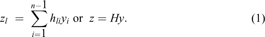
After defining the swing bus, one can calculate the flow of electricity through all the lines as a function of the injections in the other n – 1 nodes in the system. More specifically, the connectivity within the network allows one to calculate an (n – 1) × m “transfer admittance matrix,” which we denote by H. In the electrical engineering literature, a transfer admittance matrix or nodal admittance matrix, in its simplest form, is an n × n matrix describing a power system with n buses—it is simply a power flow model. Let us denote zl as the thermal limit within each transmission line, yi as the amount of electricity injected into the line from node i, and hli as an element of the H matrix. This element represents the fraction of power injected at node i that flows through line l. Given these assumptions, the total flow of line l can be expressed as:
The second term in equation (1) represents equation in matrix notation. For a more detailed explanation of the admittance matrix presented here, the reader is referred to Schweppe et al. (1988).
Equation (1) indicates the power flows through the system given any set of injections (dispatch), but it does not include thermal constraints or limits imposed on the transmission lines. If the line is at its maximal thermal limit, then dispatch is infeasible. Therefore, we define line limits as follows:

where

where
Optimal nodal pricing problem
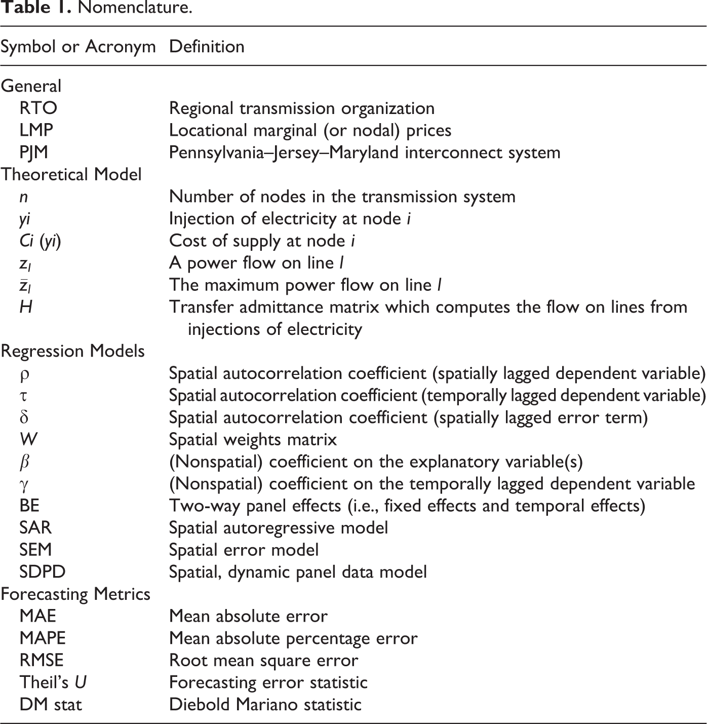
Following Schweppe et al. (1988) and Bushnell and Stoft (1996), we provide a generalized approach for computing the optimal spot prices at each node in a wholesale electricity market. To help motivate the model, we provide a definition of all the variables in Table 1.
Nomenclature.
We assume that there are clearly defined cost functions at each node in the network. We let Ci (yi ) denote the cost of supplying y megawatts of electricity at node i. Abstracting away from transmission losses, the optimal dispatch problem is
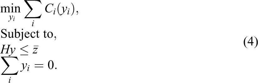
The objective function in equation (4) can be interpreted as a cost minimization problem subject to two constraints. Intuitively, the first constraint implies that the amount of electricity flowing into the lines cannot exceed the upper thermal limits of the lines. The second constraint is an expression of Kirchhoff’s Current Law, which is a statement about the conservation of energy. Formally, the law states that the vectorial sum of all currents at a node or bus is equal to zero (Behrendt, Costello, and Zocholl 2010). More intuitively, Kirchhoff’s law implies that the total charge flowing into a node must be the same as the total charge flowing out of the node. Therefore, the sum of all the currents is zero. (Please note that equations [1]–[4] do not directly incorporate Kirchhoff’s Current Law explicitly into the objective function. It is possible to do so, as in Schweppe et al. 1988. However, to keep the model tractable, we abstract away from explicit inclusion of the law into the objective function.)
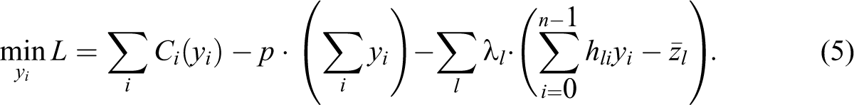
We expand the model to compute prices when transmission constraints are binding within the system. For this, we formulate a Lagrangian, and let p denote the Lagrange multiplier on the energy balance constraint (the second constraint in equation [4]) and λl denote the multiplier for the flow constraint (the first constraint in equation [4]) on line l. Given these the assumptions, the Lagrangian can be specified as follows:
The optimal solution for equation (5) is obtained by differentiating the Lagrangian with respect to the nodal injection yi :
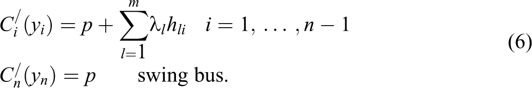
The power system depends on the flows in all the lines and thus on the net injections as represented by transfer admittance matrix in equation (3). The admittance matrix cannot depend on injections at all the nodes according to Kirchhoff’s Current Law (Kirschen and Strbac 2004). To get around this difficulty, the n bus in the system is designated as the swing or slack bus and the injection at this bus is omitted from the first equation in equation (6). Given all the other net injections in equation (6), the injection of the swing bus can be adjusted to satisfy the optimization condition (Kirschen and Strbac 2004). The concept of the swing bus is purely mathematical and has no physical implications (in terms of one node or bus in the grid system being designated as the swing bus), so the choice of the swing bus is purely arbitrary, and we have chosen bus n as the swing bus.
The Lagrange multiplier p thus represents the marginal cost or marginal benefit of an injection of power at the swing bus. In a purely competitive network of finite capacity, p represents in the nodal price at the swing bus. The nodal prices at the other buses are related to the price at the swing bus by combining the equations in equation (6):
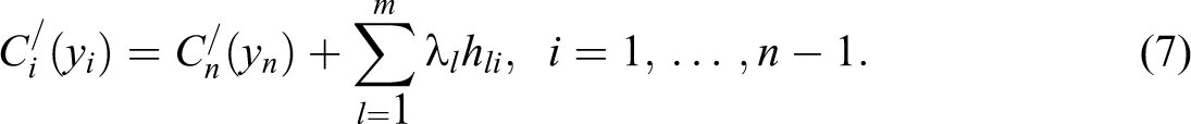
If an increase in the net injection at node i adds to losses in the system (i.e., assuming hli > 0), then

and the nodal price paid to generators at node i is smaller than the nodal price at the swing bus to penalize the generators for the additional losses they would cause by injecting an increment of power in the network at that node (Kirschen and Strbac 2004). Consequently, consumers at node i pay a lower price because an increase in load at that bus would reduce the losses. The opposite holds true if an increase in the net injection at node i reduces the losses in the system. If all losses are neglected, then the nodal prices at all buses are equal (Kirschen and Strbac 2004).
The Kuhn–Tucker necessary conditions are 3
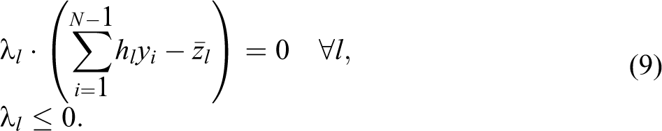
The optimal solution for the cost minimization problem, when transmission constraints are binding, implies that the marginal cost of injecting yi at any node is equal to the sum of Lagrange multiplier, p, and the constraints on the transmission lines. Another way to interpret the first Lagrange multiplier, p, is as the optimal nodal spot price, which implies that marginal costs should equal the spot price plus the constraints within the system. This implies that if independent operators had perfect knowledge, then the market clearing prices for supplying electricity within the system should reflect the theoretical spot price while taking into consideration the transmission constraints within the system. The line constraints, λ l , then can be interpreted as the shadow prices of the transmission lines within the system (Li, Liu, and Salazar 2006). These shadow prices represent the marginal benefit to the system of increasing the thermal limit on a line.
The shadow prices can alternatively be interpreted as congestion costs in the system. At times of low demand, for example, in the late evening hours, there is little or no congestion within the system (i.e., the transmission lines are not at their thermal limit), and so the shadow prices are generally negligible. Hence, during periods of low demand, the prices at each node should be nearly identical. The competing generators rely upon the transmission network to schedule and dispatch their produced electricity, and the sale of electricity is organized through spot and forward markets and through bilateral contracts with the end-use customer or marketing intermediaries (Joskow and Tirole 2000).
Bushnell and Stoft (1996) offer the important observation that the “optimal spot price” at a node is the “average of the prices at all other nodes” weighted by their relative change in supply when power is injected at that node. Although the authors’ observation is not directly obvious from the solution in equation (6) above, their statement can be understood from intuition. The solution in equation (6) is for the optimal spot price at one single node in the system. However, there are multiple nodes in the system. So as additional operators inject electricity into the system then congestion is created, which in turn make the thermal constraints binding. Therefore, if all operators behave optimally, as in equation (6), then they will consider these constraints within the system and offer a price to the ISO that reflects this information, and the price then at one node is a reflection of the average of prices at the other spatial nodes. In the current study, we use this spatial information in our empirical approach to better predict prices in a wholesale electricity market.
The correspondence between the optimal solution in equation (6) and the spatial relationship in nodal spot prices may not be immediately obvious. One of the underlying assumptions in the above optimization problem is that an alternating current (AC) is being used in the transmission network, which corresponds with empirical reality in PJM. The problem with AC is that the electrical current can move in multiple directions, and, therefore, operators cannot entirely control the flow of electricity through the grid system. An additional assumption involves the sensitivity of the flow of electricity along line l and in relation to the injection at node i—this is not necessarily explicitly modeled in the optimization problem but more on this subject can be found in Kirschen and Strbac (2004) and Stoft (2002). Solving equation (6) can be computationally difficult because it implicitly involves the solution of the power flow equations and potentially can be nonlinear (Kirschen and Strbac 2004). Consequently, the spatial dependence within the underlying system is not modeled explicitly in the optimization problem above because it would only further complicate the model. That is, the nodal price is affected by the flow constraint on a single line, the thermal constraint (represented by the transfer admittance matrix), and the sensitivity of the flow at bus m to the net injection at node i. Instead, we discuss the spatial dependence by appealing to the intuition derived from equations (7) and (8) above.
Spatially Weighted Matrix
In spatial econometrics, the spatial weight matrix is simply a compact reflection of the geographical relationship among different points in space. For example, a geographical contiguity matrix is a binary matrix with a one indicator if two points are neighbors and a zero indicator otherwise. The spatial weight matrix can be written as follows:
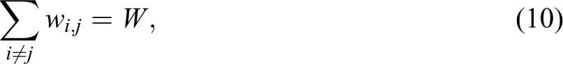
where wi,j denotes the indicator value of whether referenced point i shares some sort of neighboring relation with point j. For ease of notation, spatial weight elements can be represented as a matrix W.
There are many different specifications for a spatial weighted matrix, such as distance weighted matrix, inverse-distance weighted matrix, and k-nearest neighbors matrix. One may argue that the specification of the spatial weight matrix will substantially affect the results of the estimated spatial autocorrelation coefficient. However, LeSage and Pace (2010) demonstrate that there is little theoretical basis for this commonly held belief. Therefore, we will rely upon a simple binary continuity matrix as described above in this study.
Methodological Approach
Data
Our data consist of PJM’s “Real-time Market,” which are a spot market for current LMPs (or nodal prices) that are calculated at five-minute intervals based on actual grid operating conditions (PJM 2013). Transactions are settled hourly and PJM issues invoices to market participants monthly. PJM provides hourly aggregated values of the real-time LMPs. The LMPs then are historical values, which are listed hourly by zone for each day of market operation. For proprietary reasons, PJM takes an average of the nodal prices to represent the prices by zone. A map of the zones is provided in Figure 1 above.
In addition to the real-time market, PJM also provides a day-ahead energy market, which is a forward market for hourly LMPs that are calculated for the next operating day based on generation offers, demand bids, and scheduled bilateral transactions (PJM 2013). The day-ahead markets provide accurate price signals for market participants to make informed decisions about the next day’s market operations. For example, if there are planned outages or transmission disruptions, then such information may be reflected in the day-ahead market prices.
The participation in day-ahead electricity markets opens arbitrage opportunities for power producers. When the producer’s real-time imbalance with respect to the day-ahead contract is in the opposite direction compared to the overall system imbalance, power producers received a more favorable price at the balancing market (Morales et al. 2014). Specifically, producers can sell excess energy compared to their day-ahead position at a higher price than the day-ahead price when there is a deficit of power production in the system as a result of deviations from producers and consumers with respect to their day-ahead positions (Morales et al. 2014). Conversely, when the grid system has a surplus of power, producers can purchase their production deficit at a lower price.
Borenstein et al. (2008) and Saravia (2003) have examined the day-ahead energy market and found a spread between the day-ahead and real-time hourly price on the US power markets. Both authors attribute the spread to market power and speculative activity. In a similar study, the authors analyzed the difference between the day-ahead price and expected real-time price, the risk premium, and found that premiums are affected by demand, sales, and price variation (Longstaff and Wang 2004). Forbes and Zampelli (2011) examined the day-ahead markets in California and found that day-ahead price reflected processed information and expectations of all market participants regarding day-ahead demand. Huisman, Huurman, and Mahieu (2007) found that day-ahead prices are mean reverting, the speed of mean reversion differs by hour of day, and prices exhibited a block structured cross-sectional correlation pattern.
In this study, we collected the hourly real-time spot and day-ahead prices in the eighteen zones that existed in PJM interconnection from January 1, 2012 to October 31, 2013. For each of the 670 days in the total sample, we have downloaded price data for each of the twenty-four hours of the day from PJM website.
Regression Models
There are N = 18 cross-sectional zones, observed over T = 670 days in our data set. In this study, we will observe the estimation and prediction of each current hour. Our empirical model is

where pit
is the real-time price for the hour of the day t in the zone i, and
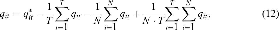
In this study, we treat the individual effect as fixed meaning that we assume that this variable is correlated with the explanatory variable and approximately “fixed” over time for each zone within the sample. If we allow for FEs terms to enter into the error term and estimate equation (11) without controlling for it, then the estimates will result in omitted variable bias (i.e., if the FE is correlated with the explanatory variables). To control for FEs we can either (1) estimate µ i and η t directly in the model by creating dummy variables for these parameters as in a least squares dummy variable model or (2) we could demean the data as in a FEs or within estimator. In this study, we use the FE estimation method. The individual and time FE can be eliminated by transforming the data as follows (Elhorst 2012):
where
Empirical Strategy
Spatial econometric models have come under criticism recently for problems associated with identification and for a lack of appeal to theoretical foundations (Partridge et al. 2012). According to these criticisms, the problem of identification is similar to Manski’s (1993) “reflection problem,” where group average characteristics (neighboring electricity prices) affect individual outcomes (local electricity prices), but the parameters in the model are not identifiable. That is, it is hard to separate out the effects of what causes prices to fluctuate locally versus what causes price fluctuations in neighboring regions.
We agree that there may be potential problems with the exogeneity of the spatial weighting matrix (among other things), so rather than appealing to causality we focus primarily on the alternative validation strategy of prediction, which is less dependent on prior theory. In other words, we take the spatial panel models as a black box and test them against empirical reality (Freedman 1991).
Given our assumptions of the spatial weighting matrix, we now demonstrate the empirical model used to identify the optimal theoretical solution provided in equation (6) above. We assume that independent operator (electricity producer) has constant marginal costs, α, so equation (6), excluding the swing bus, can be rewritten as:
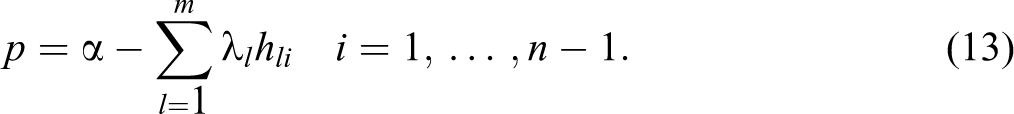
As discussed above, λ l is a parameter that represents the shadow prices of the thermal constraints within the system. Equation (13) represents how the transmission system is managed. Due to the complexity of the transmission system, it would be incredibly challenging to develop a (structural) statistical model that captures the thermal limits within the system, and it would be difficult if not impossible to acquire data on the thermal limits. However, because of the thermal constraints, we know that there are spatially dependent relationships between prices at each node in the system. One way to model these relationships is to impose a structure on these spatially dependent relations. Ord (1975) proposed a parsimonious parameterization for the dependence relations—namely, the spatially weighted matrix discussed above. In other words, the second term on the right-hand side of equation (13) can be proxied by a simple continuity spatial weight matrix. For example, we instead could use a spatial econometric model to estimate the relationship in equation (13), such as 4
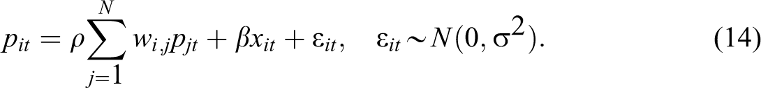
Equation (14) is a reduced-form estimable model corresponding to equation (13) or its structural counterpart in equation (6). The structure of equation (14) gives rise to a generating process known as the spatial autoregressive (SAR) process, which captures Bushnell and Stoft’s (1996) observation that the optimal nodal price at one location is a reflection of the average nodal price at neighboring locations. The spatial weight matrix then is simply a compact representation of the transmission system (as represented by the price behavior within the grid). Note that equation (14) does not explicitly capture the management aspects of the transmission system but rather implicitly captures management decisions as reflected in the price behavior of all the nodes within the system.
In addition of the SAR model, we examine different specifications of spatial econometric models as well. The grouped spatial econometric model can be written as:
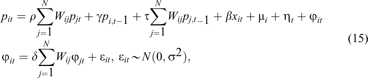
where ρ denotes the scalar SAR parameter on the dependent variable, γ is a scalar parameter on the temporally lagged dependent variable, τ is the spatial autocorrelation coefficient on the temporally lagged dependent variable, and δ is the spatial autocorrelation coefficient on the error term.
The restriction of the parameters within equation (15) defines the specific type of spatial panel data model used. The SAR model could be obtained by restricting γ, τ, and δ equal to zero—this model exhibits spatial dependence within only the dependent variable. The SEM is obtained by restricting φ, γ, and τ equal to zero—this model exhibits spatial dependence within only the error term. The spatial dynamic panel data (SDPD) model is obtained by restricting δ equal to zero—this model allows for spatial dependence within both the dependent variable and the temporally lagged dependent variable. If all the parameters except γ and β are restricted, then we derive the dynamic panel data model with FEs. Finally, if all the parameters except for β are restricted, then the model reduces to the traditional pooled OLS model with both FEs.
Note that our modeling approach differs paradigmatically from Douglas and Popova (2011) who focus on a spatial econometrics model estimated by the GMMs approach of Kapoor, Kelejian, and Prucha (2007). Further, Douglas and Popova primarily focus on a SEM specification. The advantage of the GMM approach is that it is distribution free, whereas the quasi-maximum likelihood approach, adopted here, assumes that the pricing data are normally distributed. Is this a problem for our analysis? Perhaps, but since our focus is on prediction, not causality, this is not as much of an issue. The quasi-maximum likelihood approach is based on the model developed by Yu, de Jong, and Lee (2008, 2012), and Matlab code was provided by the authors (Yu, de Jong, and Lee) for our particular application. The benefit of using maximum likelihood is that it allows us to experiment with several different spatial specification models, and the examination of the different specifications presents a contribution to the literature. The potential drawback with Yu, de Jong, and Lee’s method is that the asymptotic theory relies upon a relatively large cross section (N) and a relatively large sample along the time dimension (T). Our empirical approach has a very large sample along the time dimension but a relatively small sample (eighteen zonal regions within PJM) within the cross section. Despite this potential deficiency, Yu, de Jong, and Lee argue that when T is large relative to N, their model still produces consistent and asymptotically normal estimates. If our empirical approach were to focus more on the interpretation of parameters and make appeals to causality, then the relatively small cross-section sample may present a problem. However, since we are focusing on the forecasting ability of this particular model, the relatively small cross section should not be as problematic.
Forecasting Metrics
Three common metrics are used to evaluate forecast accuracy: mean absolute error (MAE), mean absolute percentage error (MAPE), and root mean square error (RMSE). These metrics are defined as
The symbol T denotes the total number of time periods, and N denotes the total number of zones within the system. The symbol F(t) denotes the forecasted value, and A(t) denotes the actual empirical observation. The difference between the forecasted value and the empirical observation denotes the forecast error. Therefore, the smaller the forecasted error, the better the model predicts future values. These metrics are often called ex post forecasts because the independent variables do require forecasts themselves (Greene 2003). According to Kennedy (2008), MAE is appropriate when the cost of forecast errors is proportional to the absolute size of the forecast error. MAPE is the average of the absolute values of the percentage forecast errors, and it has the advantage of being dimensionless. MAPE is more appropriate when the cost to forecast error is more closely related to the percentage error than to the numerical size of the error (Kennedy 2008). A problem with MAPE is that it often performs underforecasting. The errors in the RMSE metric are squared before averaging, so the RMSE gives a relatively higher weight to large errors—ergo, RMSE represents a “quadratic loss function.” RMSE is one of the most popular metrics in use.
Another metric for evaluating prediction is based on the Theil U statistic (Theil 1966; Greene 2003). The potential problem with the ex post forecast metrics above is that those metrics have scaling problems. The Theil U statistic is scale free and measured as follows:
The ex post forecast metric measures the “fit” of the predictive models, whereas the Theil U statistic measures how well the models perform against “naive” models, such as a random walk. The Theil U statistic is similar to the measure for R 2 (Greene 2003). With the specification in equation (19), the statistic is bounded between zero and one, and a larger value indicates poor forecasting performance. For the sake of robustness, we consider all the ex post and Theil U forecasting metrics in the current study.
DM statistic
Finally, we use a panelDM statistic (Diebold and Mariano 1995) to determine statistically if the SDPD model forecasts can be distinguished from the other forecasts. The panel version of the DM statistic was developed by Pesaran, Schuermann, and Smith (2009). The calculation of the panel version of the DM statistic is outlined in Pesaran, Schuermann, and Smith (2009), so we exclude its definition in the current study. (Our Matlab code, for the estimation of the panel DM statistic, is available upon request.)
Results
For an initial analysis, separate regressions were performed for each hour of the day of operations within the wholesale market. These regressions were performed because electricity demand varies throughout the day according to a daily load curve, which demonstrates the demand for electricity and the subsequent load in the system to meet demand. The load curves for a typical summer and winter profile are provided in Figures 2 and 3, respectively. Both figures illustrate the demand for electricity within PJM. Demand is low in the early hours of the morning, so the load in the system is relative low. Demand grows gradually throughout the day and then eventually peaks at around 7–8 p.m. in the evening. The only difference is that the winter profile has a bimodal peak, whereas the summer profile generally has a single peak. The bimodal peak stems partially from the demand for residential heating.
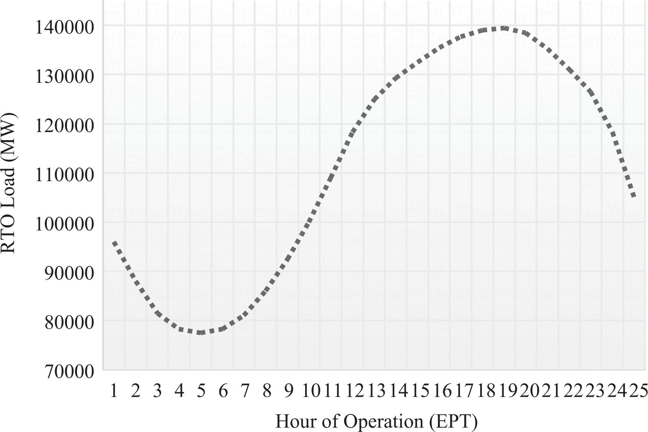
PJM daily load curve—Summer profile.
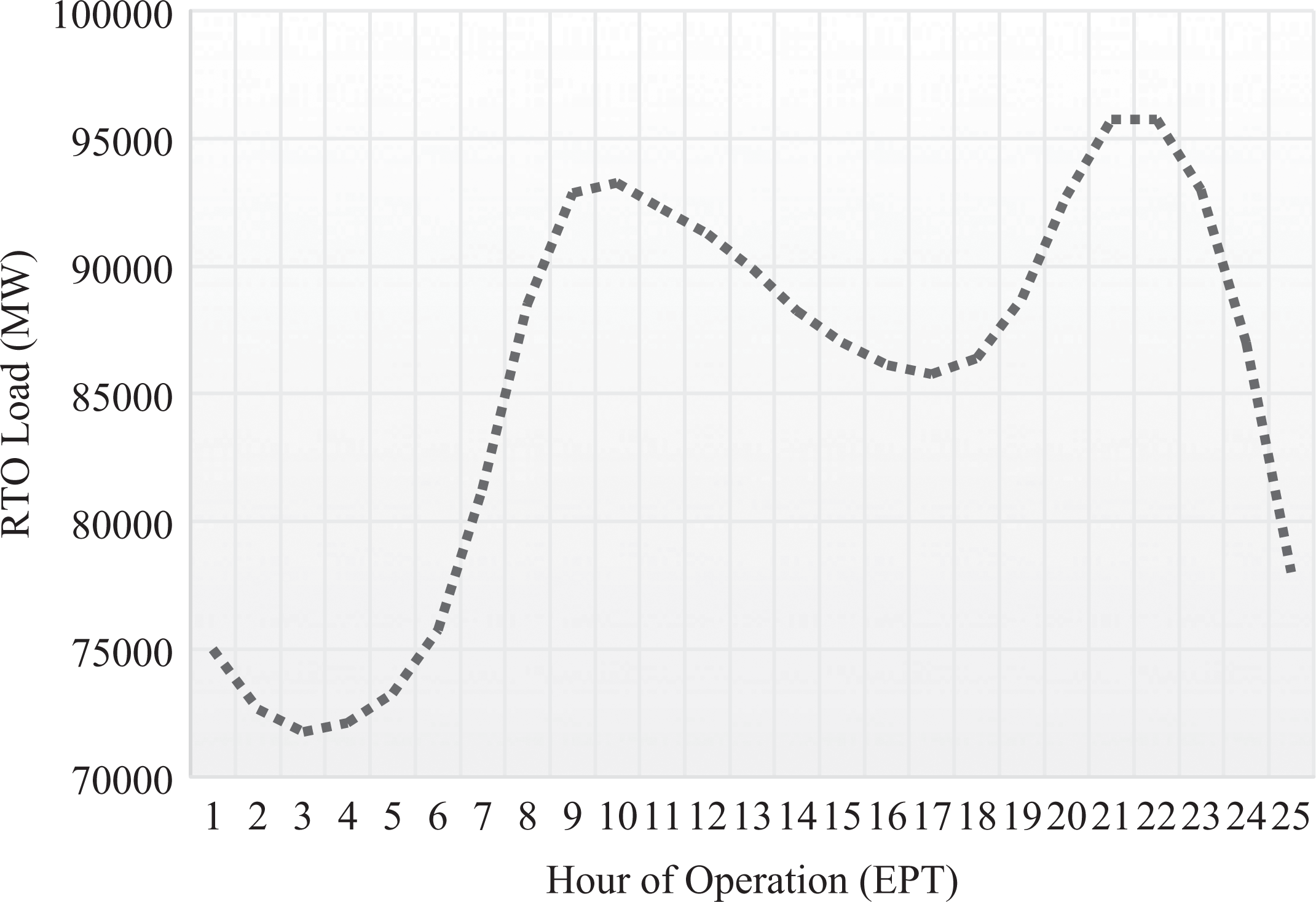
PJM daily load curve—Winter profile.
The estimation results for the different specifications of panel data models are presented in Table 2. Consistent with our expectations, the results indicate that the real-time electricity prices exhibit spatial autocorrelation for each hour of market operation. That is, the estimates of ρ in the SAR and SDPD models are positive and statistically significant at the 1 percent level. The estimates of δ in the SEM model are also positive and significant at a 1 percent level.
Estimation Results.
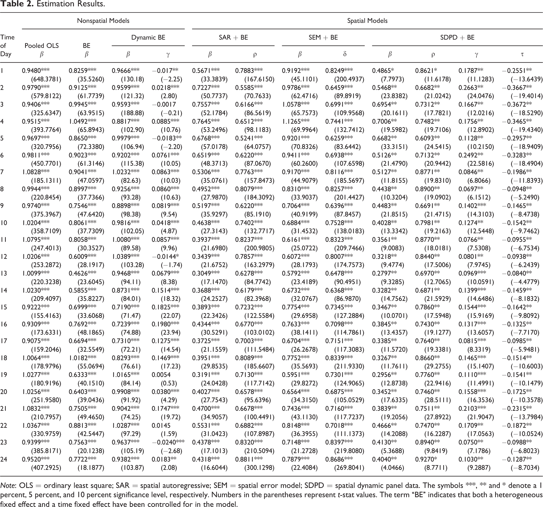
Note: OLS = ordinary least square; SAR = spatial autoregressive; SEM = spatial error model; SDPD = spatial dynamic panel data. The symbols ***, ** and * denote a 1 percent, 5 percent, and 10 percent significance level, respectively. Numbers in the parentheses represent t-stat values. The term “BE” indicates that both a heterogeneous fixed effect and a time fixed effect have been controlled for in the model.
It is worth noting that the estimates for the β coefficients are not directly comparable across the different models in Table 2. For the OLS and SEM models, the parameter estimate for β reflects the partial derivative ∂pit/∂xit (averaged over the sample of observations taken over time and space). For the SAR specification, the β coefficient implies the partial derivative ∂pit /∂xit = β/(1 – ρ). On the other hand, for SDPD model specification, the interpretation of the β coefficient is far more complicated (Debarsy, Ertur, and LeSage 2012).
An interesting result from the SDPD model is that the estimated spatial autocorrelation coefficient, τ, on the temporally lagged dependent variable is negative for each regression run by hour of the day. In the spatial statistics and econometrics literature, a positive spatial autocorrelation coefficient is associated with data values that tend to cluster together in space, whereas negative spatial autocorrelation implies that associated data values tend to disperse. Positive spatial autocorrelation is predominant in spatial data analyses.
As it turns out, the interpretation τ is actually much more complicated due to the covariance between space and time in the model (Debarsy, Ertur, and LeSage 2012; Parent and LeSage 2012). Parent and LeSage (2012) utilize a Bayesian method to estimate a dynamic, spatial data model. In their approach, they motivate the dynamic model as arising from spatial and time dependence filter expressions, which imply, using the notation from equation (15) above, that the parameter τ is approximately restricted to –ρ × φ (Parent and LeSage 2012, 728–29). This restriction is not stated explicitly in Yu, de Jong, and Lee (2008, 119), but it is implied by the reduced-form model expressed in equation (2) of their manuscript. Therefore, a simple interpretation is that our SPDP estimates yield positive spatial dependence (interpreted as the estimated sign on ρ) and positive temporal dependence (estimated sign on γ) but negative space–time covariance (estimated sign on τ). A further discussion of the interpretation of negative space–time covariance is beyond the scope of the current study; however, additional information can be found in Parent and LeSage (2012). For a general discussion of negative space–time covariance, additional information can be found in the statistical mathematics literature in Gregori et al. (2008).
Based on the estimation results for the full sample of data, it would seem that the spatial econometric models could improve the accuracy of predicting the LMPs relative to the nonspatial models. Due to the lack of direct comparability of the β coefficient estimates across the different models, Table 3 displays the reduced-form parameter estimates based on the approximations outlined in the preceding paragraph. To derive the approximate reduced-form estimate for β in the SDPD model, we calculated it as ∂pit/∂xit = β/(1 – ρ – γ – τ).
Approximate Reduced-form Parameter Estimates for β Across the Different Models.
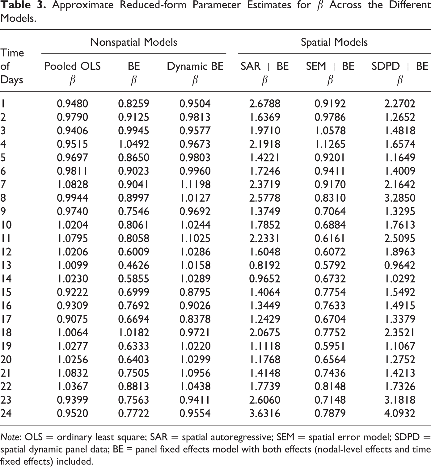
Note: OLS = ordinary least square; SAR = spatial autoregressive; SEM = spatial error model; SDPD = spatial dynamic panel data; BE = panel fixed effects model with both effects (nodal-level effects and time fixed effects) included.
In general, it seems that the pooled OLS model is underestimating the effect of β, whereas the SAR and SDPD models yield much larger estimates for β. More specifically, the SAR model estimate is approximately 90 percent larger than the OLS model estimate, on average across the different time periods, and the SDPD model is approximately 92 percent larger on average. We will demonstrate in the next section that the SDPD model yields the smallest forecast errors; therefore, it seems that the models that do not account for spatial autocorrelation within the dependent term underestimate the effect of β. The SAR model, which does account spatial dependence but ignores temporal dependence, perhaps slightly underestimates β based on the forecasting error. The SDPD model, which accounts for spatial and temporal dependence and space–time covariance, arguably yields the most accurate estimates as it provides the smallest forecasted errors. To further test the validity of spatial panel data models, we compare the forecasting performance of these models against empirical reality in the next section.
Forecasting Results
In order to carry out the forecasts, we shorten the full sample of observations by omitting the last s days of observations, where s denotes different prespecified lengths of time. Specifically, we will explore three out-of-sample specifications: (1) short term (s = one week), (2) the medium term (s = one month), and (3) the near term (s = three and six months, respectively).
We define the s number of observations as the “out-of-sample” observations. Note that we still observe the last s number of observations, only we exclude these observations from the regression so that can use the s observations to compare against forecasted values over the same period. In other words, we run regressions on the shorter “within sample” and then use the forecasts against empirical reality to see which model provides the best predictions for the out-of-sample data.
We compute the prediction for the ith individual zone at a future period t + s, in which t is the number of days within sample, t + s is the total number of days of full sample, which equals 670. The term s denotes the number of days for the forecasting period. The forecasts are conducted by regressing the model on the entire initial within sample, and then forecasting over the entire out-of-sample period using the empirical observations of the independent variable within the out-of-sample period.
We used our PJM price data set to calculate and compare the accuracy of pooled OLS, nonspatial FEs, dynamic panel data model with FEs, SAR, SEM, and SDPD forecasts. The results of the forecast error performance, in the context of MAE, MAPE, RMSE, and the Theil U statistic, of each of the models are presented in Tables 4–7. Weron and Misiorek (2007) forecast electricity spot prices with a series of Gaussian and heavy-tailed innovations to improve the power of the forecasts. In the current study, we did not experiment with heavy-tailed innovations because it would significantly complicate the estimation of the spatial econometric forecast models. Instead, we leave such extensions for future research.
Short-run Forecast Metrics for the First Half-day of Business Operation.
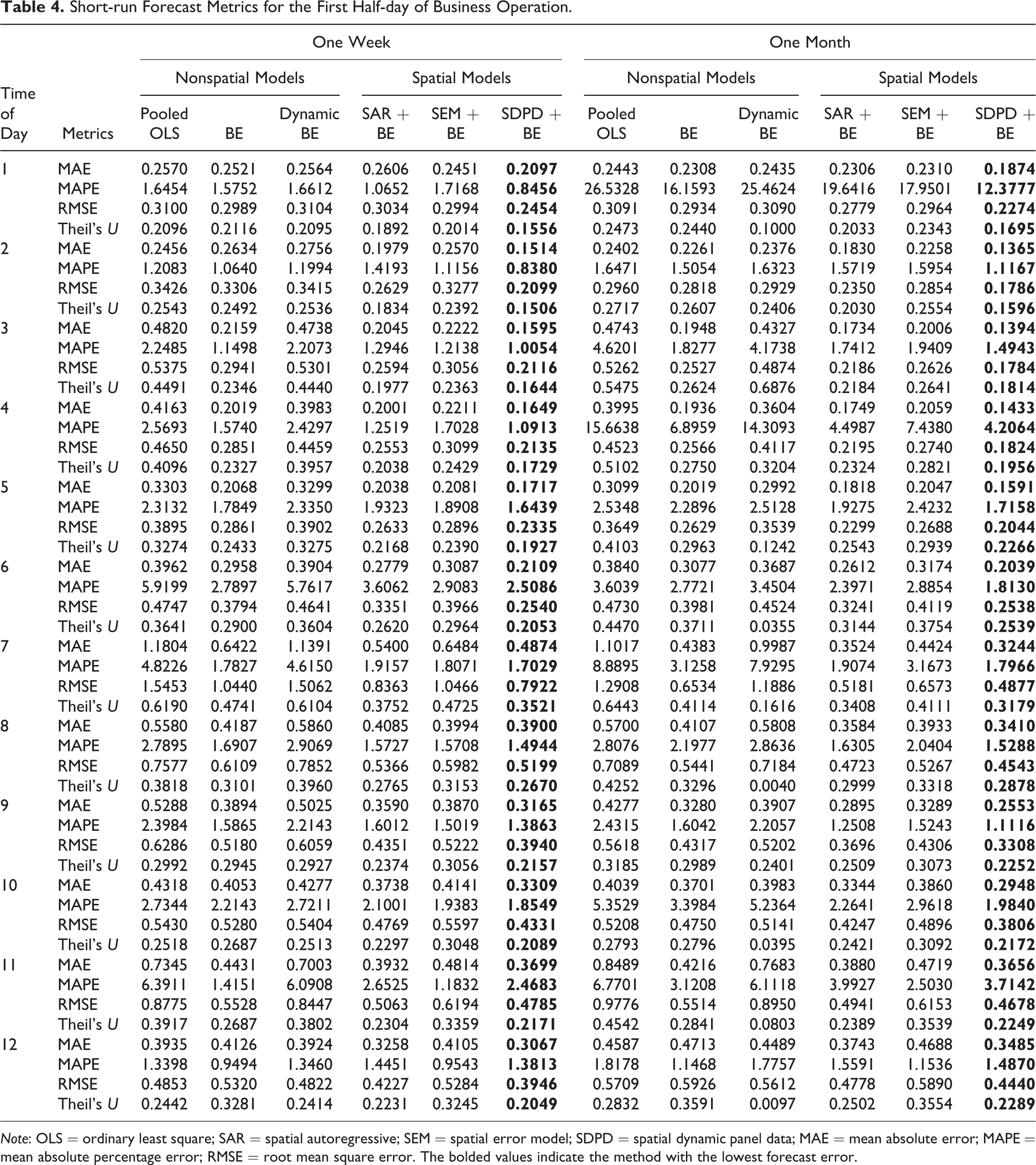
Note: OLS = ordinary least square; SAR = spatial autoregressive; SEM = spatial error model; SDPD = spatial dynamic panel data; MAE = mean absolute error; MAPE = mean absolute percentage error; RMSE = root mean square error. The bolded values indicate the method with the lowest forecast error.
Short-run Forecast Metrics for the Second Half-day of Business Operation.
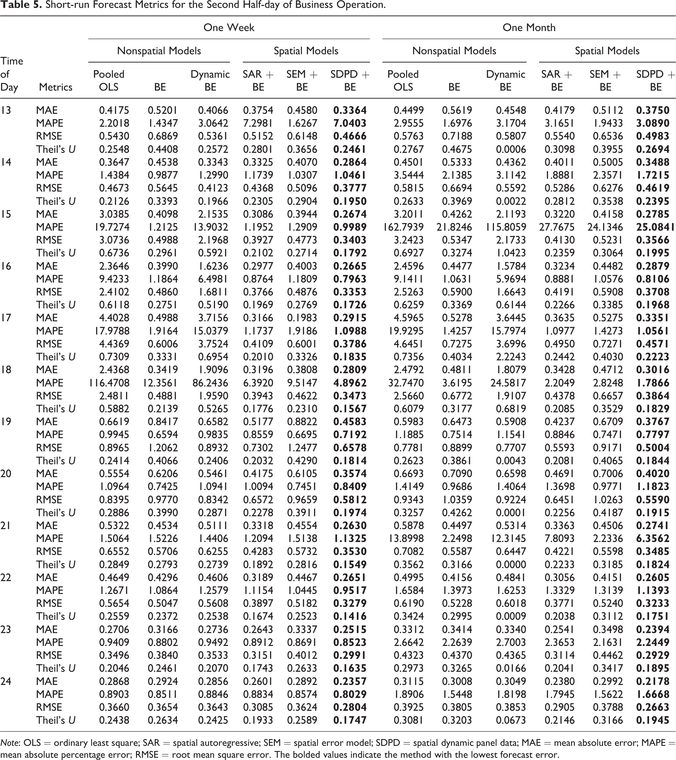
Note: OLS = ordinary least square; SAR = spatial autoregressive; SEM = spatial error model; SDPD = spatial dynamic panel data; MAE = mean absolute error; MAPE = mean absolute percentage error; RMSE = root mean square error. The bolded values indicate the method with the lowest forecast error.
Medium-run Forecast Metrics for the First Half-day of Business Operation.
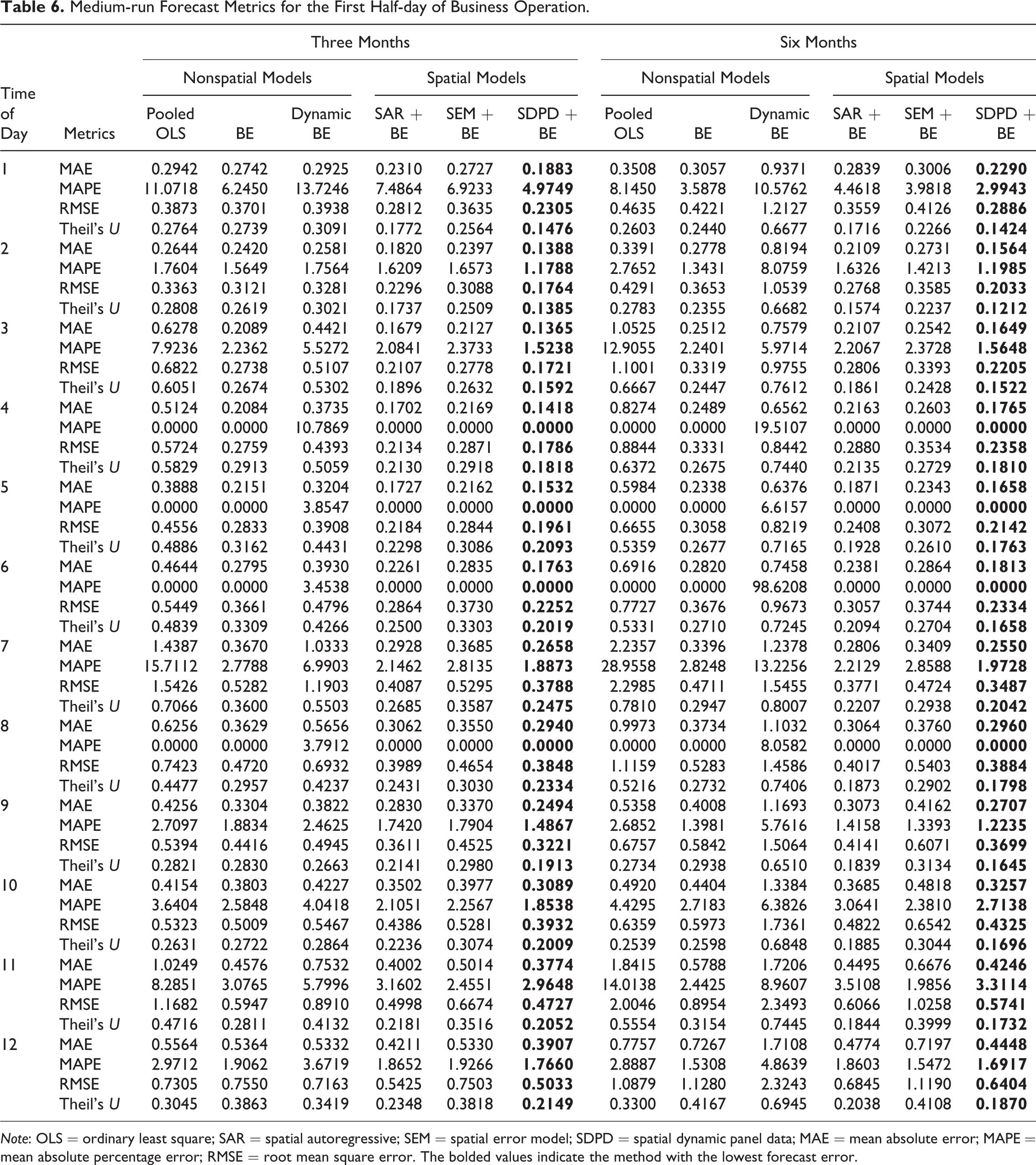
Note: OLS = ordinary least square; SAR = spatial autoregressive; SEM = spatial error model; SDPD = spatial dynamic panel data; MAE = mean absolute error; MAPE = mean absolute percentage error; RMSE = root mean square error. The bolded values indicate the method with the lowest forecast error.
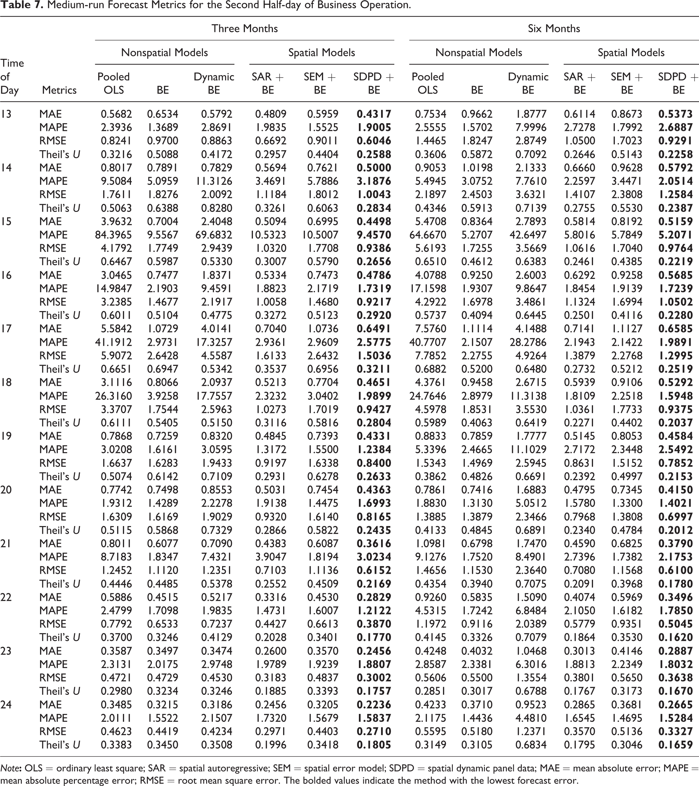
Medium-run Forecast Metrics for the Second Half-day of Business Operation.
Note
Based on the forecasting error metrics in Tables 4–7, it is clear that the SDPD model provides the best forecasts across all of the different specifications, times of day, and forecast window. This can be observed by recalling that the smaller the forecast error, the better the forecasting ability of the particular estimator. However, the small forecasting errors of the SDPD model are not necessarily indicative of superior predictive ability, unless the SDPD model forecasts are statistically different from the other models’ forecasting errors. Therefore, we next turn to the panel DM to statistically test the difference in forecasts between the SDPD and the other models.
In order to accurately estimate the panel DM statistic, we restrict its calculation to one-week-ahead forecasts to reduce the chance of having serial correlation within the underlying data, which could possibly invalidate our ability to infer from the DM tests. We made no adjustments for serial correlation because we are only forecasting seven days in advance; therefore, it is reasonable to assume that the differentials are serially uncorrelated. For forecasts greater than seven days, the panel DM statistic can be modified to deal with the serial correlation by using a Newey–West type estimator. We do not pursue this extension here. According to Pesaran, Schuermann, and Smith (2009), the degree of cross-sectional dependence of the forecast errors has to be sufficiently weak for
Diebold Mariano Statistics for the Spatial Dynamic Panel Data Model Relative to a Select Number of Benchmarks.
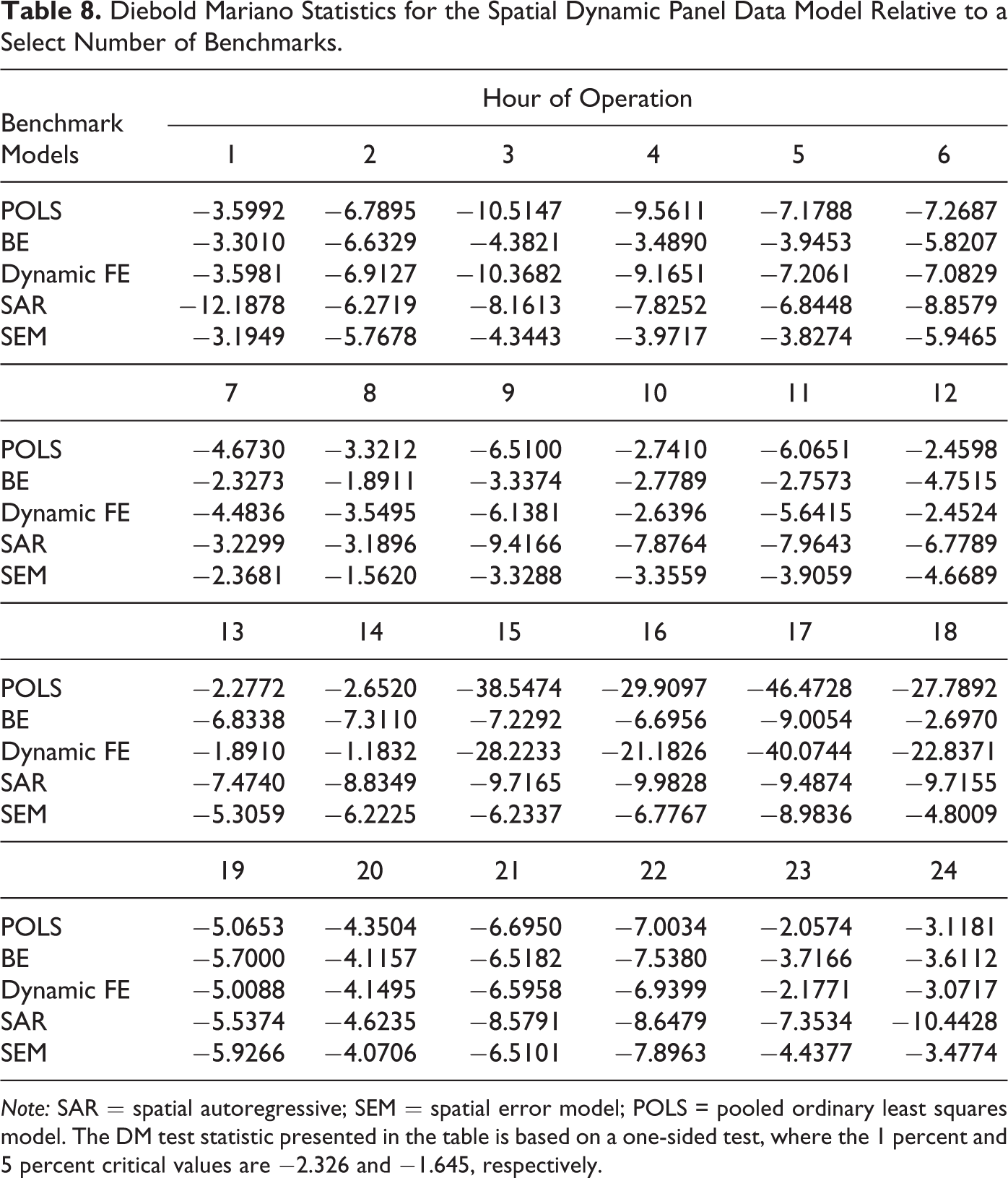
Note: SAR = spatial autoregressive; SEM = spatial error model; POLS = pooled ordinary least squares model. The DM test statistic presented in the table is based on a one-sided test, where the 1 percent and 5 percent critical values are −2.326 and −1.645, respectively.
The results of the panel DM tests largely corroborate the findings in Tables 4–7. That is, the DM test results imply that the spatial dynamic panel model provides forecasts that are statistically distinguished from the benchmark forecasts at conventional significance levels. The only exception is for the one-week forecasts for the fourteenth hour of operation during the business day. During that time, the forecasts of dynamic FEs model cannot be statistically distinguished from the dynamic panel data model with FEs. These tests also seem corroborate our claim that the SDPD controls for congestion within the transmission grid, which leads to a spatial relation in the spot prices. This is revealed through the fact that congestion increases during peak demand. Table 8 reveals that the SDPD forecasts are highly statistically distinguished from the benchmarks models during peak demand (fifteenth to twenty-second hours of operation).
Discussion
We were able to exploit the geographic nature of the transmission system within PJM interconnection to better predict near-term and medium-term zonal spot prices. Arguably, these zonal prices display spatial autocorrelation because of congestion within the transmission system. Using a simple engineering model, we derived the optimal nodal pricing strategy for an independent generator within a whole electricity market. The engineering model demonstrated that a cost-minimizing operator would consider not only marginal costs but also the shadow price of the thermal limits within the transmission system. Due to these shadow prices, the spot price at one zone will be affected by the spot price in neighboring zones. Consistent with the observations of Bushnell and Stoft (1996), we used a spatial econometric model as a reduced-form model that accounts for the shadow prices within the system. Our within-sample empirical results indicated that spatial autocorrelation is indeed present in the zonal spot prices. The dynamic, spatial panel data model offered the best predictions, in a forecasting error context, of the zonal spot prices in the near and medium term.
Conclusions and Policy Implications
Market operators can use spatial econometric models to better predict short-term and near-term zonal or nodal spot prices. From a generator standpoint, this can improve price offerings and trading strategies by using the spatial autocorrelation as a proxy for the shadow price of transmission constraints.
Based on our findings, the policy implications for the regional transmission organizations, such as PJM, are potentially far reaching. LPM theoretically is based on the producer’s marginal cost and the transmission constraints within the system (i.e., the shadow price), as we demonstrated above. However, real-world conditions within the grid system diverge from the idealization of the underlying theory. Therefore, it is useful to examine the ways in which real-world electricity markets diverge from the underpinning theoretical models. The spatial econometric model we laid out was capable of approximating the thermal constraints within the transmission system by using the spatial weight matrix as the reduced-form expression of such constraints, and thus, our empirical approach constitutes a relatively simple model of network optimization. We demonstrated that the dynamic, spatial panel model provided the best predictions of zonal price across a range of different near-term and medium-term scenarios. As the spatial weight matrix is a relatively easy method to model system constraints, central operators may use such information to improve current market operations such as better predicting demand and supply. PJM currently uses alternative approximations and proxy estimates of constraints based upon mathematical optimization and the operator’s knowledge of historic system operations (Hausman et al. 2006). One could argue that the spatial weight matrix approximation (at the base of the spatial econometric model) is far too simple of an approximation. However, the spatial econometric model provides a useful comparison to evaluate the system operator’s existing approximation scheme. This comparison is consistent with FERC’s (1997) explicit goal to produce efficient, accurate economic signals that would spur investment in both electricity market infrastructure and demand response programs. Implicit with this goal, and consistent with the purpose of deregulation in the markets, is the potential to reduce market power and enhance competitiveness. Therefore, the approach outlined in the article can potentially be used to evaluate PJM’s (and other RTOs) current LMP operationalization to help ensure that it enhances competitiveness and benefits customers.
The evaluation of current RTO’s operations and market performance is important because the Government Accountability Office issued a 2008 report stating that FERC had not conducted an empirical analysis to measure whether RTOs have achieved their expected benefits (GAO 2008). In response to GAO’s (2008) report, FERC issued a set of performance metrics in 2010; however, the American Public Power Association (2011) criticized the metrics as insufficient and argued that FERC’s final approved performance measures were similar to those recommended by the RTOs themselves. Our methodology and findings cannot provide a comprehensive assessment an RTO’s performance, but as outlined above, our approach can be used as alternative means to test an RTO’s formalization of LMPs.
System operators of restructured markets could potentially use the models and analysis presented within this article to better design wholesale electricity markets. In the near future, the operations of RTOs will likely be seriously impacted by ever increasing penetrations of variable renewable generation, such as wind and solar energy. The characteristics of variable generation will present challenges to RTO market design as greater variability and uncertainty in generation and dispatch will require additional reserve capacity (Smith et al. 2010). Smith et al. (2010) argued that renewable energy generators may have profit motives to continue operating during periods of moderately negative LMPs. Renewable generators put downward pressure energy prices as their marginal cost is near zero. Several market operators, including PJM, allow renewable generators to submit negative price offers, this allows generators (such as wind turbine operators) to offer prices at which they are willing to reduce output in the system. Thus, renewable penetration will create additional pressures on operators to not only possibly redesign the markets but also to constantly monitor and forecast demand and supply throughout the day to ensure grid stability. The models and analysis presented in this article can aid the operators in forecasting supply and demand.
This study was limited by the available data. PJM, for proprietary reasons in many cases, has aggregated the nodal prices to zonal prices. Aggregating to the zonal level is easier for the construction of the spatial weighting matrix, but a great deal of the spatial granularity within the grid is lost by aggregating to the zonal level. Bjørndal and Jørnsten (2001) argue that zonal prices are second best (from an economic welfare perspective) compared to optimal nodal prices. Walton and Tabors (1996), on the other hand, posit that the difference in prices within zones is very small, and the only discrepancies are caused by line losses between nodes within the same zone. They argue that the within zone system is essentially unconstrained, so the short-run marginal cost at nodes within the zone will always be nearly the same but may vary together on an hour-by-hour basis. Therefore, this study may have arguably benefited by using nodal prices and subsequently greater detail within the topology of the transmission grid, which would lend itself to a more detailed spatial weighting matrix. However, since the spatial econometric model(s) were able to better predict the zonal prices, our results may suggest that the spatial dependency between nodes extends beyond the current zonal boundaries. This finding merits further research as to whether the zonal boundaries accurately reflect the congestion boundaries within PJM and other wholesale electricity markets.
Footnotes
Declaration of Conflicting Interests
The author(s) declared no potential conflicts of interest with respect to the research, authorship, and/or publication of this article.
Funding
The author(s) received no financial support for the research, authorship, and/or publication of this article.