Spatial Heterogeneity in Amenity and Labor Market Migration

Abstract

The disequilibrium and equilibrium models of migration disagree on how local amenities and labor market dynamics influence regional in-migration. Research into migration motives and decision-making show that migration for some individuals is mainly driven by proximity to the labor market, while migration for others is mainly amenity driven. As this is an ongoing process, it should result in a spatial sorting based on migration motives. This means that global models explaining in-migration underestimate the influence of both factors through averaging out of the coefficients across these diverse regions. In this article, we compare a local and a global model explaining in-migration through residential quality and labor market proximity. We find significant differences in the influence of the explanatory variables between regions. Demonstrating this spatial heterogeneity shows that the impacts of factors underpinning migration vary across regions. This result highlights the importance of the regional context in anticipating and designing regional policy concerning population dynamics.

Keywords

residential quality labor market population change spatial heterogeneity disequilibrium model of migration equilibrium model of migration

One can identify two underlying causes of internal migration destination choices (cf. Morisson and Clark 2011; Partridge 2010; Storper and Scott 2009). On the one hand, disequilibrium models explain migration primarily through the spatial restoration of a labor market equilibrium (Storper and Scott 2009). Equilibrium models, on the other hand, argue that there is a trade-off between labor market utility and utility derived from amenities which determines the eventual location choice (Morisson and Clark 2011; Partridge 2010).

In this article, we take the driving mechanisms on in-migration from both these approaches, labor market growth and amenities, and assess whether their influence is spatially homogenous across the Netherlands. There are strong empirical indications that the connections between these two factors and in-migration might exhibit spatial heterogeneity: in some areas, labor market opportunities may be important for attracting in-migrants in spite of a lack of amenities, whereas in other areas the prospect of a higher quality of life could be more important in attracting in-migrants, even if labor market opportunities are sparse.

Existing studies suggest that migration to cities, for instance, is primarily driven by access to the labor market. In fact, urban migration is mostly studied from a disequilibrium type of approach (see Storper and Scott 2009; Crozet 2004). Similarly, studies into rural migration generally employ quality-of-life measures as explanatory factors for the growth or regeneration of rural regions (Beale 1975; Stockdale 2006; Halfacree 2008). Migrant flows to rural areas, such as counterurbanization, are composed of those people who can afford to trade proximity to labor market opportunities for a higher level of amenities in their living environment (Gosnell and Abrams 2011; Partridge 2010). Furthermore, the distinction in the importance of factors on in-migration is not necessarily one of urban opposing rural. Empirical evidence increasingly points to more diverse spatial patterns of amenities and labor market growth as drivers of migration. Bijker, Haartsen, and Strijker (2013), for instance, show that not all rural areas are attractive, and there is a significant discrepancy between the types of people who move to popular or less-popular rural areas, and their motives for migrating. Similarly, in the urban context, Clark et al. (2002) find that amenities play an important role in urban growth processes, and Florida (2002) identifies more specific attributes related to amenity-driven urban growth.

Another difficulty related to the study of amenity migration is the operationalization of the concept of amenities and consequently amenity-rich and amenity-poor regions. Amenities as a concept are hard to define, and many contemporary studies resort to using proxy-based measures consisting of spatial attributes assumed to contribute to a better environment: Florida (2002), for instance, uses urban elements such as theaters and an open, Bohemian and tolerant society as a proxy for urban amenities, whereas rural qualities such as lakes and mountains are used in counterurbanization studies (Moss 2006).

People, however, do not rate environmental attributes similarly. There are differences between socioeconomic groups (Bourdieu 2010). Moreover, these differences extend to within groups and to the point that changes in spatial preferences can be observed within an individual at different stages in the life course (Boyle, Halfacree, and Robinson 1998). This means that the operationalizing amenities through objective measures does not account for a proportion of amenity moves motivated by different sets of amenities to those used in the operationalization, while also misidentifying some moves not motivated by amenities.

This study contributes to the existing literature by taking the heterogeneity in migration motives and patterns as its starting point. Such an approach involves accounting for the whole migration system, not just interurban or urban to rural migration. Migration motive research shows that migration flows are characterized by different motives for moving and consequently involve different people (Boyle, Halfacree, and Robinson 1998; Niedomsyl 2011). These different motives for migration result in a sorting mechanism, where people select their destination region based on their personal preferences (cf. Bijker, Haartsen, and Strijker 2013). This sorting mechanism predicts that certain regions will be more attractive to persons for whom proximity to the labor market is more important, while other regions will be more attractive to persons for whom residential quality takes precedence over labor market proximity. Consequently, the correlations between in-migration and these factors will vary between regions. Such an approach requires the inclusion of the whole migration system (not only interurban or urban–rural) and requires that interpersonal differences in the relevance of amenities are accounted for in the operationalization of amenities.

In this study, we attempt to compare the explanatory potential of the labor market and residential quality in explaining in-migration by analyzing regional differences in the importance of these factors attracting migrants for the whole of the Netherlands. To do so, we incorporate regional variations in the importance of the labor market and amenities through a local, spatially heterogeneous, regression—a mixed geographically weighted regression (mGWR; Fotheringham, Brunsdon, and Charlton 2002), while including personal variations in the valuation of amenities. By using an mGWR, we can test for spatial heterogeneity in the model in order to establish if the correlation between labor market growth (and likewise for amenities) and in-migration is constant across all regions or whether the coefficients display spatial variation.

By studying the factors underpinning the attraction of new residents, we contribute to a further understanding of the question what attracts migrants. Establishing if there are regional differences in drivers of in-migration is of particular relevance within the current context of population decline (Haartsen and Venhorst 2010) and for policy makers attempting to deal with issues related to population decline.

Theory

Migration Models

The disequilibrium model of migration

There are several distinct migration theories with different outcomes regarding the spatial distribution of population (for an overview, see McCann 2013). Of these theories, the most prominent current debate is between the disequilibrium and the equilibrium models of migration. The disequilibrium model of migration develops from neoclassical theories predicting that people migrate as a response to a disequilibrium in regional labor demand and supply functions (Harris and Todaro 1970). The theory states that if there is a discrepancy between the labor supply and demand between two places (the disequilibrium), people will move from where the supply of labor is relatively higher to the place where the demand of labor is relatively higher, thus restoring the equilibrium (cf. McCann 2013). As a result, regions experiencing an increase in labor market opportunities should see positive net migration (although the direction of causality in this particular issue is still debated; Hoogstra, van Dijk, Florax 2011).

Proponents of the theory (see Storper and Scott 2009) argue that the disequilibrium model of migration is successful in explaining agglomeration from the origins (although not the locations) of cities through to present-day metropolitan regions. The model also predicts an optimum, or equilibrium, which can be shown to be efficient from the perspective of the economy as a whole (McCann 2013). Opponents of the theory, however, argue that the formal predictions of the disequilibrium model fail to account for some of the more prominent contemporary migration flows, including the resurgence of population growth in amenity-rich locations and counterurbanization (Partridge 2010).

The equilibrium model of migration

The equilibrium model of migration states that people can elect to offset returns on labor and lower prices of tradable goods by better access to nontradable goods, in this case, amenities in order to maximize personal utility. In areas with high levels of amenities, the real wage can therefore be lower while still offering the population the same utility as areas where low levels of amenities are compensated through higher wages (McCann 2013).

In support of the equilibrium models, research into migration motives shows evidence supporting amenities as playing at least some role in migration destination selection. The observed nature of population flows reveals that a (labor market driven) central tendency is not equally applicable across regions. In developed countries, once basic household provisions are met (Graves 1979), scholars have identified various migration flows involving people moving away from city centers, such as suburbanization and later counterurbanization (McGranahan, Wojan, and Lambert 2011), next to the predicted flows toward urban concentrations. Explanations of these migration patterns tend to focus on a combination of the pull of amenity-rich areas away from city centers as well as the push of urban disamenities such as crowding, crime, and congestion (Findlay, Short, and Stockdale 2000; Gregory et al. 2009). Similarly, in urban research, the “creative class” theory, for instance, highlights the importance of urban amenities in attracting human capital and fostering economic development (Florida 2002). It seems that for both urban and rural areas, the quality of the living environment plays an important role in the selection of the migration destination region.

Storper and Scott (2009) argue against the amenity-driven migration proposition, stating that the theory is too reliant on ad hoc explanations of migration phenomena. In addition, the theoretical model is limited to those people who can afford to choose amenity-rich locations over labor market dynamics, constraining the explanatory power to affluent people (at the individual level) and developed regions (at higher levels of aggregation). Amenity-driven migration therefore fails to explain the origin of cities or to make predictions with regard to future migration patterns.

Personal Preferences and Migration

Studies into migration show there are differences in the importance of amenities relative to the labor market in the individual migration decision. These differences are related to a person’s position in the life course (see Boyle, Halfacree, and Robinson 1998) but also to various characterizations of socioeconomic status (Venhorst, van Dijk, and van Wissen 2010). Regional labor markets are not all equal in their effect on in-migration. Underlying motives for moving change over one’s life course. For instance, students move toward university cities for education (Faggian and McCann 2009), graduates are more likely to move to or between urban centers (Krabel and Flöther 2014; Venhorst, van Dijk, and van Wissen 2010), while moves later in the career show that the importance of labor market proximity diminishes relative to the quality of the living environment (see Bijker and Haartsen 2012; Stockdale 2006).

Bijker, Haartsen, and Strijker (2013), for instance, find a complicated mix of underlying motives and consequently distributions of people. Rural areas which fit more closely to a “rural idyll” (see Amcoff 2000; Hjort and Malmberg 2006) attract people with higher educational attainment, or upper-middle-class persons, who belong to the traditional counterurbanization groups, whereas the composition of the migration flow to less popular rural regions is very different and more reliant on social network motives (Bijker, Haartsen, and Strijker 2013). Within the wider construct of rurality, rural areas differ in terms of who they attract both in urban to rural migration and in rural to rural migration. Similarly, there are differences between urban areas regarding amenities and which people they attract (Clark et al. 2002).

This spatial heterogeneity in the importance of different types of amenities implies that using standard global statistical models, such as ordinary least squares (OLS), will not be able to correctly identify the correlations (Fotheringham, Brunsdon, and Charlton 2002). For instance, if a certain set of amenities in one region plays a role in attracting migrants, but not in the other, there is the potential that coefficient estimates from a global model will be incorrectly identified as not significant (averaged out between the region with, and the region without a significant effect), leading to type II errors. In terms of equilibrium/disequilibrium discussion, this could lead to the incorrect identification of labor market factors as the dominant pull factor in migration destination selection.

Spatial Implications

The two dueling models predict very different spatial outcomes of migration patterns. On the one hand, the disequilibrium approach suggests that in the short-term labor market, dynamics will drive migration and in the longer term predicts a central tendency toward complete agglomeration (provided there are low transport costs; Partridge 2010). Importantly, the disequilibrium model has a solution (the equilibrium) at any given regional distribution of labor supply and demand and predicts that labor market growth will lead to population growth.

On the other hand, the equilibrium approach has no single solution, as personal preferences toward amenities differ from one individual to the next (McCann 2013). This means that the spatial outcome of the equilibrium approach is dependent on individual preferences. Life cycle and life-course approaches do indeed confirm that locational behavior is dependent on personal preferences, which in turn change along the life course (Boyle, Halfacree, and Robinson 1998). As a consequence, no single spatial outcome can be predicted.

Data and Model Specification

Spatial Heterogeneity in Migration

The overview of the literature on the influences of amenities and the labor market on migration in Personal Preferences and Migration and Spatial Implications subsections suggests that these influences are spatially heterogeneous. Regions with labor market opportunities are more attractive for a specific subset of the population, and the same goes for areas which are high in amenities. This implies that the marginal effect of the labor market or amenities on in-migration will not be constant over space. Previous studies have not been able to capture these spatially varying relationships. The spatial variation cannot be captured through global statistics like an OLS regression. In estimating global statistics, this spatial variation can lead to underestimation of the effect or errors in estimating the significance due to the averaging out of the effects across space (Fotheringham, Brunsdon, and Charlton 2002).

Unlike an OLS, a GWR does not assume that the effect of the explanatory variables is constant across space. A GWR solves this problem by estimating local coefficients for each area. This is accomplished by estimating a series of local regressions for a predefined number of nearest neighbors for each area and weighting the values of the neighbors by their distance to the target area (for a complete overview of GWR, see Fotheringham, Brunsdon, and Charlton 2002). The benefits of taking this approach are that locally significant effects are identified because the effects of the right-hand side (RHS) variables are allowed to vary spatially. By allowing a spatial variation in the estimation of the effects, a GWR can identify whether the correlations between the labor market and amenities and in-migration vary across the study area.

Model Specification

Left-hand side (LHS) variable: in-migration

For our analysis, we look at the sum of in-migration into municipalities in the Netherlands collected by Statistics Netherlands (Centraal Bureau voor de Statistiek [CBS] 2014b) over the study period (2006–2012). We follow Ostbye and Westerlund (2007) and Fratesi (2014) who argue that analyzing gross migration statistics is more reliable since a small or zero net migration could still hide a regional redistribution of human capital (see also Rogers 1990). To eliminate the effect of population churn, which would result in larger in- and out-migration flows for larger municipalities and could obscure the effect on in-migration under investigation, the numbers of in-migrants are standardized per 1,000 inhabitants in the municipality at the starting year of the study period. In our study, we focus on the attraction of migrants into regions, meaning that gross in-migration is the appropriate variable.

RHS variables: the labor market

We attempt to explain the crude in-migration rate per municipality between 2006 and 2012 through labor market opportunities and the residential quality of the neighborhood. As a proxy for labor market opportunities within the functional labor market, we use growth in the number of residents receiving an income in a municipality for the period 2006–2012 (CBS 2014b). The persons receiving an income includes all individuals who received an income in the previous fifty-two weeks (including unemployment benefits, pensions). For the purpose of this study, we modified the existing variable, excluding individuals receiving pensions, unemployment benefits, and disability benefits.¹ Using this proxy allows us to estimate the growth in number of jobs reachable from a household’s residence rather than using a spatially lagged variable based on the number of jobs per municipality. Therefore, by estimating the number of residents receiving an income in a given municipality, we incorporate the functional labor market within the variable, since commuters are also accounted for.

RHS variables: amenities

One of the main issues with models incorporating amenities as a factor in the migration destination selection process is that there are large discrepancies in definitions of amenities and their operationalization. Among the broadest definitions, Partridge (2010, 7) defines amenities as “simply anything that shifts the household’s willingness to locate in a particular location.” The problem with such a broad definition is that, although it can be argued that this better captures the holistic nature of the concepts involved, it does impose empirical problems (de Chazal 2010). As a consequence, studies into the subject apply a variety of concepts (such as quality of life, livability, and environmental quality) and an even wider variety of definitions, often blurring the distinction between the operationalization and the definition of the concept (for an overview, see van Kamp et al. 2003).

One of the main problems with research into amenities is developing a relevant empirical strategy (van Kamp et al. 2003) that accounts for varying personal preferences and valuations of different types of amenities. General theories like the creative city or rural idyll (Florida 2002; Partridge 2010; Van Dam, Heins, and Elbersen 2002) struggle to incorporate individual differences in the valuation of amenities. In both concepts, a single set of amenities (i.e., green space, rural living, outdoors, etc.) is formulated to explain the migration flows. However, individual migration motives differ and personal preferences dictate the relative importance of amenities.

Self-reported measures of satisfaction are increasingly used in studies dealing with environmental attributes and noneconomic factors (cf. Van Praag and Baarsma 2005; MacKerron and Mourato 2008; Brereton, Clinch, and Ferreira 2008). Self-reported measures are, however, not without their complications. Individual variations in the valuation of different options on the satisfaction Likert scales could lead to problems with interpersonal comparisons as well as questionnaire context issues such as item placement. Much of the research into the validity of self-reported satisfaction considers life satisfaction or well-being in general. Pavot et al. (1991, see also Pavot and Diener 1993) find evidence that individual assessments of well-being are comparable to peer-reviewed assessments of well-being, meaning that different individuals use similar constructs of well-being. This means that assessments of well-being between persons are comparable. Their study also deals with the item placement issue, showing reliable results for single-item well-being data and only a very small or insignificant effect of item placement.

For the purpose of our study, we use residential satisfaction with the living environment collected by WoON (WoonOnderzoek Nederland [Residential Survey the Netherlands]) (Ministerie van Binnenlandse Zaken en Koninkrijksrelaties [BZK], CBS 2013; Ministerie van Volkshuisvesting, Ruimtelijke Ordening en Milieubeheer [Ministry of Housing, Spatial Organisation and the Envirnonment] 2005). The WoON data set is composed of a three-yearly survey commissioned by the Dutch ministry of internal affairs to assess housing quality and housing preferences and includes a subsection on the residential environment. These data are collected at the individual level and aggregated to the municipal level as a proxy for amenities. The municipal level is the lowest level of spatial aggregation for which the respondent’s location data are available. In order to average the underlying Likert data to aggregate municipality scores, the individual items are assumed to be equidistant from each other. The averaging of the data is necessary for the variable to be included in the model, but violation of the equidistance assumption in the data could be problematic. Given the interpersonal validity of well-being data (Pavot et al. 1991), we do not expect this assumption to be a problem.

The question in the survey is (on a five-point Likert scale), “How satisfied are you with your residential environment?” The questionnaire does not specify what is meant by residential environment, but in the questionnaire, it is preceded by a section on the satisfaction with the dwelling and followed by a section on satisfaction with neighborhood-level interventions, implying a spatial scale between the dwelling and the neighborhood. The precise interpretation of the residential environment is left to the discretion of the respondent.

Following Balestra and Sultan (2013), we argue that residential satisfaction is an outcome variable for those aspects that influence a resident’s valuation of the residential situation. Using individual self-reported residential quality instead of a predefined set of characteristics means the different personal preferences are included in the variable itself. Combined with the utility model specified by Partridge (2010), we argue that an increased valuation of the residential situation correlated with higher in-migration constitutes amenity migration.

Control variables

First, we control for the urban–rural residential satisfaction effect identified by Sorensen (2013) by adding a dummy variable for degree of urbanization (CBS 2014a; categories 1 and 2: urban municipalities have 1,500 addresses or more per square kilometer). This dummy will help control for the discrepancy in experienced residential quality between urban and rural areas. Given that rural areas generally have higher residential quality than urban areas and that the overall tendency of migration flows is still toward urbanization, failing to control for the urban–rural difference means that residential quality will function as a measure of rurality.

Second, we control for agglomeration effects derived from larger population sizes by adding the log-transformed density per municipality. This measure captures the effect of agglomeration that relatively large municipalities have, even in areas with no urban center. Given that the optimal bandwidth (see Model calibration and identification strategy subsection) is relatively small, the log of the density allows us to control for agglomeration effects beyond just the urban dummy.

Third, we include a dummy variable for university cities to account for the large number of students that universities attract.

The main model we estimate is:

I_{i} = β_{0} (u_{i}, v_{i}) + \sum_{z = 1}^{n} β_{z} (u_{i}, v_{i}) {(L, R)}_{i z} + β_{g} G + e_{i},

where I is the sum of the crude in-migration per 1,000 inhabitants for the period 2006–2012 at location i, β₀ is the local estimator of the intercept, L is the labor market growth per municipality, R is the residential quality in the municipality, and G are the three globally estimated variables, namely, the rural–urban, university cities dummies, and the agglomeration effect control variable.

Model calibration and identification strategy

For this study, we choose an adaptive bisquare specification of the spatial weights matrix. The adaptive approach can cope with the heterogeneity in the size of municipalities in the Netherlands, so that in the case of large contiguous municipalities, the bandwidth will widen to allow for enough data points in the regression. Using the bisquare modeling means that after a certain threshold (the bandwidth), the spatial weight of the data points equals zero.²

The optimal bandwidth for the model is determined by running a series of models with bandwidths varying from all municipalities (414) down to twenty-five at intervals of ten, decreasing the interval to one when approaching the minimum. We then choose the model which has the lowest Akaike’s information criterion (AICc) score (Fotheringham, Brunsdon, and Charlton 2002), in this case at fifty-three nearest neighbors (Figure 1). The AICc provides a numerical estimate for the distance between the estimated model and the unknown true model, and it accounts a penalty for the model’s complexity. If the AICc score of one model is sufficiently lower than the other (with three generally held as the threshold), the model with the lowest score is to be preferred (Fotheringham, Brunsdon, and Charlton 2002).

Figure 1.

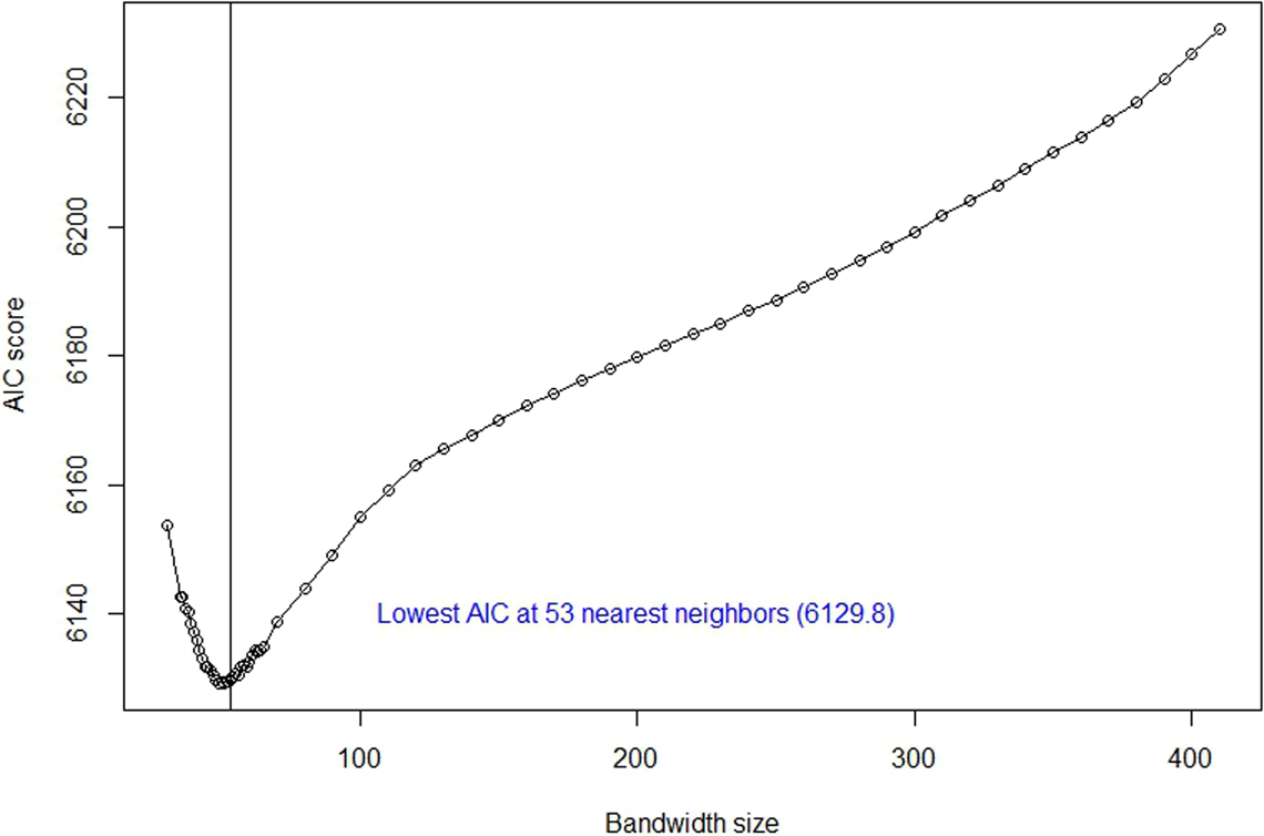
Akaike’s information criterion model calibration.

To test for the assumed spatial variability, we follow the approach as employed by Fotheringham, Brunsdon, and Charlton (2002) and Nilson (2014). First, we estimate the model as a standard OLS and map the residuals. We analyze if the residuals display spatial clustering through a Moran’s I analysis. If the residuals are found to be clustered, we have reason to believe that incorporating a spatial component into the model could improve the estimation.

Second, we estimate the same model in a GWR (using the GWmodel package in R, Version 1.2-5, by Lu et al. 2015). Since the estimates of the coefficients are now the result of local regressions, we compare the AICc for the GWR with the AICc for the standard OLS and see if the explained variance in the GWR is sufficiently greater in order to justify adding the complexity of estimating the coefficients locally. We also check if the local estimation of the coefficients of the individual explanatory variables can be justified through an improvement in the AICc (similar to Nilson 2014).

Data and Study Area

Given the precondition of affluence in order for equilibrium-type migration patterns to occur (Partridge 2010), a relatively high level of development (or affluence) is required in the study area to compare the equilibrium and disequilibrium models of migration. The data used in this article are from the Netherlands, which meet the affluence requirement. In addition, the Netherlands has a very rich set of data at low levels of spatial aggregation (415 municipalities) collected through Statistics Netherlands (CBS). One of the island municipalities (Schiermonnikoog) did not have residential quality data available, meaning this municipality is omitted from the analyses. The municipalities range in population size (2006) from 1,130 to 743,100, with a mean of 39,450 and a median of 25,060. The distribution is positively skewed, with most municipalities in the lower ranges of population size, and four main population centers in the metropolitan west of the Netherlands (Amsterdam, Rotterdam, Utrecht, and The Hague) have population sizes of over 250,000.

The municipal level plays an important role in housing policies and labor markets (Knoben, Ponds, and van Oort 2011) and represents the smallest spatial scale at which national data are available. In addition, previous studies indicate that the effects of spatial factors influencing the quality of the living environment are largest close to these factors (distances smaller than a kilometer) but remain significant for areas up to seven kilometers (Daams, Sijtsma, and van der Vlist 2016). This result shows that a low level of spatial aggregation is necessary for capturing differences in residential quality. Similarly, for the labor market, studies find that labor market effects are largest in close proximity to the area where the change in the labor market occurs, but the effects extend over a large geographical area (Hoogstra, van Dijk, and Florax 2011). In this study, we use the municipal level of spatial aggregation since it will allow us to accommodate small-scale differences in residential quality and changes in the labor market without isolating these effects from their larger spatial areas of influence.

Within the Netherlands, similar to many other developed countries, there are within-country differences in terms of population growth (Delfmann et al. 2014; Haartsen and Venhorst 2010), providing the necessary variance in the in-migration variable. The main regions expecting population decline are found in peripheral areas of the Netherlands, whereas the urban centers continue to grow. This is in line with the differences in labor market growth between urban and rural regions (Table 1). The relatively small difference of 2.35 percentage point can be explained by the fact that as a proxy for functional labor markets, the number of residents receiving an income per municipality was used. This means that labor market growth in a city will also affect the labor market growth in the surrounding (rural) municipalities and, because it more accurately accounts for the functional area, average out the urban–rural differences.

Table 1.

Descriptive Statistics.

Variable	Urban (n = 76)	Rural (n = 338)
Variable	Mean (SD)	Mean (SD)
Residential satisfaction	4.01 (0.14)	4.20 (0.17)
Labor market growth	9.04 (5.80)	6.69 (5.31)
In-migrants per 1,000 inhabitants	299.16 (82.10)	243.19 (63.18)

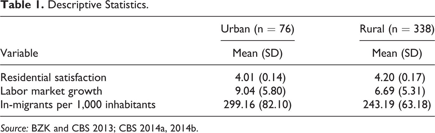
Source: BZK and CBS 2013; CBS 2014a, 2014b.

However, the proximity of perceptually rural areas in the Netherlands (Haartsen, Groote, and Huigen 2003) combined with relatively large functional labor markets and good transport networks (Hoogstra, van Dijk, and Florax 2011) should enable counterurbanization. Rural residents are more satisfied with their living environment (Table 1), which is in line with findings across the European Union (Sorensen 2013). On the surface at least, relative numbers of in-migrants appear not to respond to this discrepancy in amenities.

Results

Data Exploration

Figure 2 and Table 2 show the correlations between the variables used in this article. The correlation between residential satisfaction and the log of the density is negative, reflecting the urban–rural differences found by Sorensen (2013) and the need to control for this effect (see Control variables subsection). The other notable correlation from this initial analysis is the positive correlation between the log of the density and the standardized in-migration, showing that even after standardization by inhabitants, in-migration is higher for more densely populated municipalities.

Figure 2.

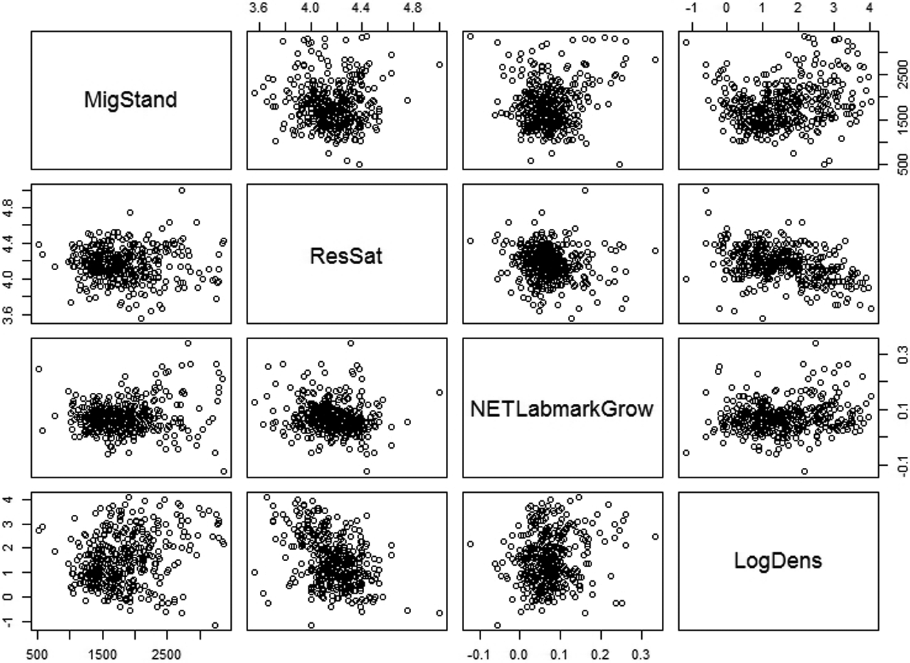
Pairwise correlations migration (standardized), residential satisfaction, labor market growth, density (log).

Table 2.

Correlation Matrix Main Variables.

Variable	Migration (standardized)	Residential satisfaction	Labor market growth	Density (log)
Migration (standardized)	1	−0.029	0.143	0.254
Residential satisfaction	−0.029	1	−0.140	−0.416
Labor market growth	0.143	−0.140	1	0.144
Density (log)	0.254	−0.416	0.144	1

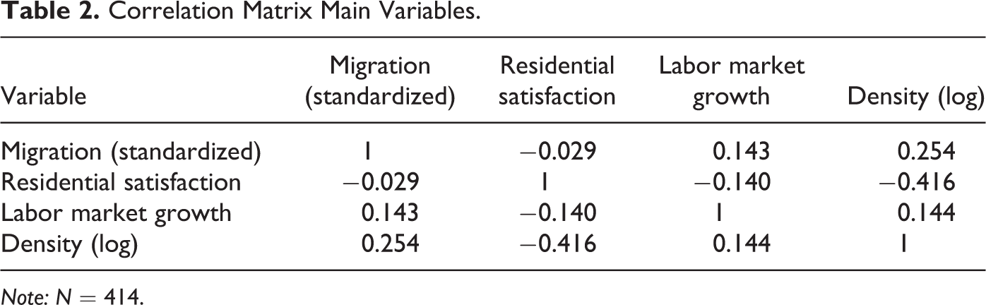
Note: N = 414.

Other notable results from the correlation matrix are relatively weak correlations between labor market growth and in-migration as well as a weak and negative correlation between residential quality and in-migration. Both weak correlations are in line with the expectation of spatial heterogeneity in the links between in-migration and labor market on the one hand, and residential quality on the other hand, meaning that differences in the size and possibly sign of the correlations average out across the study region.

Model Estimation

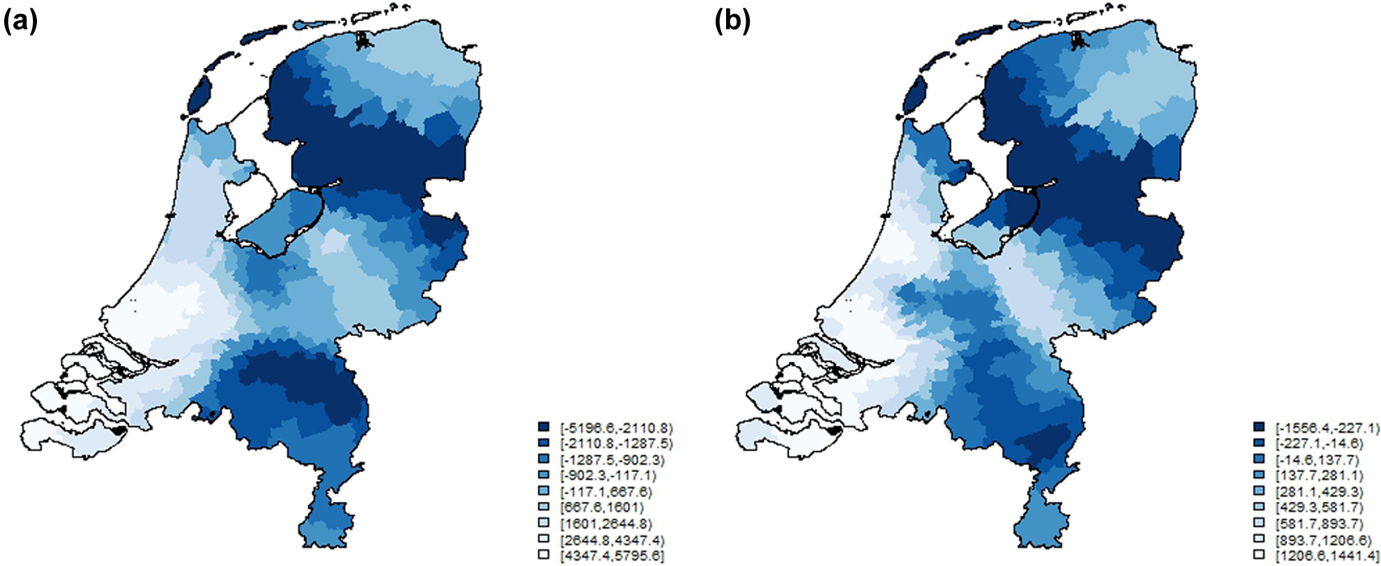
As outlined in Model calibration and identification strategy subsection, we first run an OLS and show the residuals (Figure 3a; model overview in Table 3). The Moran’s I cluster analysis shows a significant positive spatial clustering of the residuals for the OLS. The clustering of the residuals shows that in some regions, the model predominantly underestimates in-migration (such as in the northeast of the Netherlands), and in others, the model predominantly overestimates in-migration. This violates the requirement that the residuals of the OLS are independent and suggests that the model is not accounting for a spatial process present in the data, which could be explained through the spatial sorting process and resultant regional differences in the proportion of migration that can be explained through residential quality or labor market growth.

Figure 3.

(a) Ordinary least squares residuals. (b) Geographically weighted regression residuals.

Table 3.

OLS and GWR Results.

Variable	OLS		GWR			Test for spatial variability
Variable	B (SE)	T (Est/SE)	Low	Median	High	AICc difference
Residential quality	410.9 (139.4)	2.95	−18.0	321.0	723.5	−2.38
Labor market growth	7.9 (4.2)	1.86	−1,284.1	371.3	2,275.9	−14.17
Urbanization (dummy)	291.5 (84.6)	3.45		314.1 (75.5)
University (dummy)	352.7 (147.1)	2.40		302.8 (124.9)
Log density	52.5 (31.4)	1.67		33.9 (36.8)
Intercept	−107.5	−0.18	−1,285.4	385.4	1,737.0
	OLS		GWR
R ²	.13			53.8
AICc	6,258.6			6,129.8

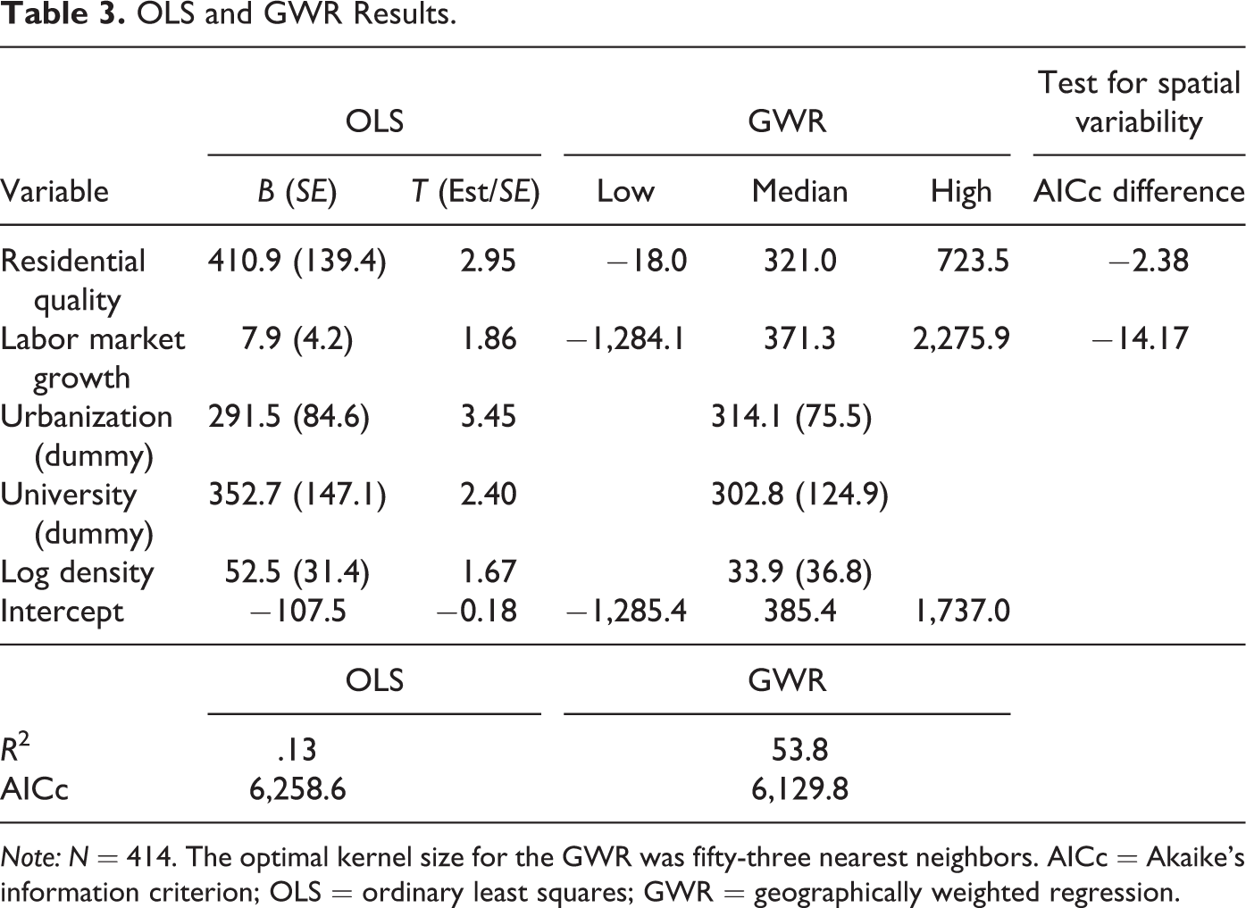
Note: N = 414. The optimal kernel size for the GWR was fifty-three nearest neighbors. AICc = Akaike’s information criterion; OLS = ordinary least squares; GWR = geographically weighted regression.

As Fotheringham, Brunsdon, and Charlton (2002) state, the clustering of residuals is a first indication that the OLS is not accounting for spatial heterogeneity in the results. Following Fotheringham, Brunsdon, and Charlton, we then run a GWR and perform the same analysis (Figure 3b). The change in the Moran’s I of the residuals from a significantly positive clustering of the residuals to no significant clustering of the residuals suggests that the GWR adequately solves the problem of misspecification of the OLS, which is a second indication of spatial heterogeneity in the relationships.

Comparing the AICc scores for the GWR and the OLS (Table 3), we see that the GWR performs significantly better than the OLS. The improvement in the AICc shows that the complexity introduced in the model by allowing the coefficients to vary spatially is offset by a more substantial improvement in the explanatory power of the model. In addition, we find that the R ² increases from .13 in the OLS to .54 in the GWR (median local value).

Looking more closely at the results from the OLS, we see that labor market growth is not a significant predictor of in-migration, while residential quality has a positive effect. The R ² of the OLS model is predictably low, consistent with the low pairwise correlations, and in line with the theory suggesting that a spatial heterogeneous estimation would provide a better fit.

In the test for spatial variability, we see that both the residential quality and the labor market growth score negative results. This means that the AICc for the GWR estimate of the explanatory variable is lower than the AICc for the alternative (fixed slope) model. This shows that the correlations between in-migration and both labor market growth and residential quality are spatially heterogeneous, and, therefore, global models are unfit for analyzing both labor market growth and residential quality and their link with in-migration. Relating back to the research question, these results show that the links between residential quality, the labor market, and in-migration are indeed spatially heterogeneous.

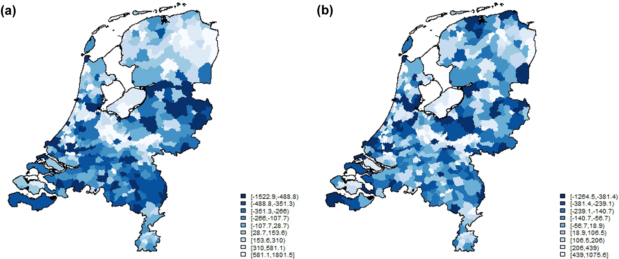
Figure 4a and b displays the spatial variability of the coefficients of labor market growth and residential quality. Since the GWR estimates regional variations in coefficient, the results shown in these maps are the local values of these coefficients, coefficient surfaces. The darker areas show a negative correlation between the LHS variable, in-migration, and the RHS variable, labor market growth (Figure 4a), or residential quality (Figure 4b), whereas the lighter areas suggest a positive correlation.

Figure 4.

(a) Coefficient surface labor market. (b) Coefficient surface residential satisfaction.

Due to the construction of the GWR (estimating local regressions at each data point in the sample), the results represent a series of tests of the same hypothesis (see Byrne, Charlton, and Fotheringham 2009). This means that the locally estimated t-statistic for the coefficients shown in Figure 4a and b needs to be adjusted accordingly. We employ the Benjamini and Yekutieli procedure (2001) controlling for false discovery rates, since this also accounts for the expected local dependence of the estimates of the GWR (Tobler 1970). The false discovery rates are obtained through the fdrtool package version 1.2.15 (Klaus and Strimmer 2015).

The results are presented in Figure 5a and b for the main variables under consideration. In this figure, the dark gray areas correspond with areas with a significant and negative coefficient and the light gray areas correspond with significant and positive coefficients. In-migration in the Western part of the Netherlands correlates positively with labor market growth mainly in the southern part of the metropolitan area. This is in line with the specification and analysis of the disequilibrium model and findings listed in Storper and Scott (2009), where the population in metropolitan regions grows in response to labor market growth. However, it does not negate the hypothesis of the equilibrium model of migration, since the utility function specified by Partridge (2010) allows for labor market migration in addition to amenity-driven migration. Indeed, throughout the metropolitan Randstad, in-migration correlates positively with residential quality. The coefficient for residential quality is positively correlated with in-migration around the national park of the Veluwe (in the center of the Netherlands) and negatively correlated around the area of Zwolle. The coefficients for labor market growth are significantly negative in rural areas in the south of the provinces of Drenthe and Fryslân and on three of the Dutch Wadden islands (Figure 4a and b).

Figure 5.

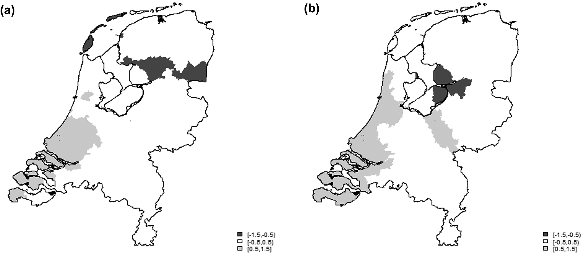
(a) Positive and negative significant coefficients for labor market growth. (b) Positive and negative significant coefficients for residential quality.

Local regressions are known to be sensitive to local collinearity (Wheeler and Tiefelsdorf 2005) even if the variables do not display such issues globally. To check for these, the local condition numbers of the cross-product matrices can be examined. Although the adaptive bandwidth measure is applied in this study (Brunsdon, Charlton, and Harris 2012), we check the local condition numbers for any problematic values. Belsley, Kuh, and Welsch (2005) establish that any values over thirty are problematic, while Brunsdon, Charlton, and Harris (2012) maintain a stricter number of twenty. Figure 6 shows the local condition numbers for our model, with darker areas corresponding with low condition numbers and lighter areas with higher condition numbers. The map shows that local condition numbers do vary across the Netherlands, with the eastern areas of the Netherlands showing up particularly high. However, the local condition numbers mostly stay below 10 (and do not exceed 10.3), showing that local collinearity should not be a problem. Figure 7a and b shows the local VIF scores with dark blue corresponding with low VIF scores and light areas with higher VIF scores, and although the spatial pattern is slightly different (regions in the north and south score higher), the local VIF scores are all in the acceptable range (lower than three). The only notable exceptions are the VIF scores for the log of the density control variable in the metropolitan west of the Netherlands which are very slightly above 3.

Figure 6.

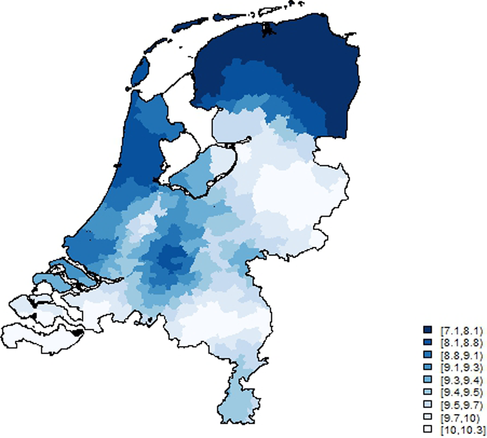
Local condition numbers.

Figure 7.

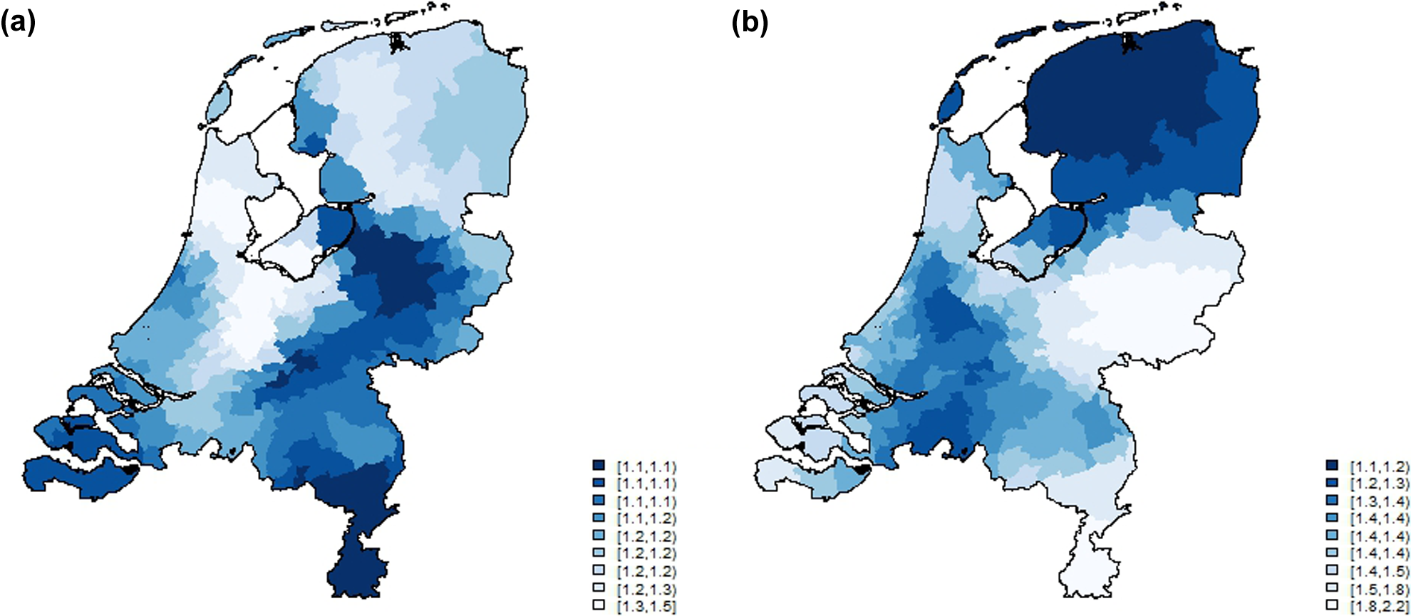
(a) Local Variance Inflation Factor (VIF) labor market growth. (b) Local VIF residential quality.

Endogeneity

In our article, we operationalize amenities through residential satisfaction in order to prevent subjecting our results to a predefined set of characteristics associated with the quality of the living environment (see RHS variables: amenities subsection). This does, however, invoke the possibility that the residential satisfaction is influenced by in-migration. One example could be that the residential satisfaction is negatively influenced by the advent of newcomers or conversely positively influenced by a perceived revival of an area. We test for this process by adding the difference in residential satisfaction between 2006 and 2012 to the model. If certain areas were more welcoming to newcomers, and others more hostile, we would expect to see a significant improvement in the AICc in the test for spatial variability. In our test, the score for spatial variability shows a positive outcome (difference in AICc = 22.8), meaning the correlation is not spatially heterogeneous, and we can reject the idea of more welcoming or more hostile regions. In addition, we tested whether in-migration correlated with residential satisfaction in a mixed GWR. Estimated globally, the difference in residential satisfaction is insignificant (t = .89). Both globally and locally estimated, the difference in residential satisfaction is not correlated with the simultaneous in-migration, meaning that the original model specification is not influenced by either a negative or a positive effect of newcomers in the area.

Metropolitan Effect on In-migration

The presence of the four major urban centers in this region combining to a metropolitan region could mean that the processes of in-migration are inherently different for this region. This could mean that in the mGWR test for spatial heterogeneity, the spatial differences are merely a reflection of a metropolitan versus nonmetropolitan dichotomy. To test for this unobservable metropolitan characteristic, three additional GWR models were run with a metropolitan dummy (one with just the two western provinces of Noord-Holland and Zuid-Holland; one with three provinces, the original two and Utrecht; and one with three provinces, the original two and Zeeland). For all three models, the metropolitan dummy is insignificant. The models were rerun without the urban dummy in the original model, given the similarity of the urban and metropolitan dummy. This did not change the results. We can therefore reject the hypothesis that there is an unobservable metropolitan effect in the Western Netherlands influencing the results in the original model.

Conclusion

In this article, we investigate the spatial heterogeneity in factors influencing in-migration. The disequilibrium model of migration predicts that, since migration is the spatial restoration of a labor market disequilibrium, labor market growth correlates positively with migration. However, the competing equilibrium model of migration argues that choosing a close proximity to amenities represents a trade-off between amenities and returns to labor (Partridge 2010). This means that returns to labor is one of a number of factors influencing migration, with the other factors grouped under amenities. Furthermore, on smaller spatial scales, empirical evidence shows that the importance of amenities and labor market considerations is not homogenous between people (Bijker and Haartsen 2012). From this, it follows that people driven by different migration motives select different regions, which in turn implies that the importance of labor market characteristics as well as of residential quality (or amenities) in migration destination selection varies across regions (cf. Niedomsyl 2011; Storper and Scott 2009). However, most empirical work consists of smaller qualitative studies exploring in depth the place-based differences (see, e.g., Bijker and Haartsen 2012) or large-scale quantitative work focusing on macro processes but sacrificing within-region variation (c.f. Crozet 2004).

In this study, we synthesize these two approaches by accounting for both the regional variations in the importance of each factor in migration destination selection, while running a nationwide analysis in a nationwide study. We estimate the correlation of labor market growth and amenities with in-migration through a GWR. This method allows us to estimate local variations in the importance of the influence of labor market characteristics as well as the influence of residential quality on regional in-migration. A particular focus of this study is to examine whether there is spatial heterogeneity in the influence of labor market characteristics and residential quality as a proxy for amenities.

The results in this article underline the theoretical assumptions and small-scale qualitative work in that it shows that allowing for spatial variability in the explanatory variables significantly improves the estimated model. These findings suggest that there is significant spatial heterogeneity in the importance of residential quality as well as of labor market growth in explaining regional in-migration, even within a small country such as the Netherlands. Especially in the northern, eastern, and south eastern part of the Netherlands, the results of this study show that there are variations in how the explanatory variables affect regional in-migration.

The results from our article show that in analyzing the spatial patterns of migration across the Netherlands, the processes attracting migrants are not constant across regions. The study does not address the question of what determines the variations in sign and size of the coefficients, this is left for further research.

This study expands on research into attracting in-migrants in three ways. First, contrary to traditional regional studies of in-migration, in our study, we allow for spatial heterogeneity in the importance of factors influencing migration. Second, while allowing for this variation, we maintain a nationwide study area. By not limiting our study to, for instance, interurban or rural–urban migration, we can test for variations across as well as within different types of regions providing a more complete picture of within-country migration. Third, in this study, we use a self-reported measure of amenities, rather than predefined spatial elements. In doing so, we improve the estimation of regional amenities allowing for a more accurate analysis of the spatial variations in the importance of (experienced) amenities.

From a policy perspective, the heterogeneity in the correlation between labor market growth, residential quality, and in-migration (including negative correlation coefficients) identified in our study shows that debates on regional population growth and population decline require allowing for the region’s specific context. This could suggest that a place-based approach toward regional growth policy in general, and population change more specifically, may be appropriate in many cases.

The spatial heterogeneity demonstrated in this article opens up several avenues of research. As mentioned before, this article does not address the underlying causes of the heterogeneity in determinants of in-migration. Answering the question why residential quality in certain regions is positively related to in migration and negatively in other regions is a logical next step in research that would also help informal local policy makers understand which regional factors contribute to in-migration.

Furthermore, the current study deals with residential quality and the labor market at an aggregate level (the municipality). As stated in Personal Preferences and Migration subsection, differences in individual (or household) socioeconomic status and position in the life course are known to affect the valuation of environmental characteristics and the utility derived from them. Extending the current model to include individual factors such as household composition, level of education (changes in), employment status (Venhorst, van Dijk, and van Wissen 2010), life course events (Boyle, Halfacree, and Robinson 1998), and levels of aspiration (Stutzer 2004) could foster a better understanding of interpersonal heterogeneity of factors determining migration destination selection.

Finally, this article deals with the migration destination selection with a focus on the destination region. A further extension of the current model could be the estimation of a spatially heterogeneous Poisson model including both origin and destination data, allowing for the control of spatial interaction effects (see Dennett and Wilson 2013). Controlling for spatial interaction effects would provide further insights into the determinants of migration-related population growth in study areas containing large differences in population sizes.

Footnotes

Acknowledgments

The authors would like to acknowledge the financial support from the University Campus Fryslân. The authors would also like to thank the National Centre for Geocomputation at Maynooth, particularly Chris Brunsdon and Martin Charlton for the feedback received.

Declaration of Conflicting Interests

The author(s) declared no potential conflicts of interest with respect to the research, authorship, and/or publication of this article.

Funding

The author(s) received no financial support for the research, authorship, and/or publication of this article.

Notes

References

Amcoff

2000. Samtida bosattning pa svensk landsbygd. Uppsala, Sweden: Uppsala Universitet.

Balestra

Sultan

. 2013. “Home Sweet Home: The Determinants of Residential Satisfaction and Its Relation with Well-being.” OECD Statistics Working Papers, 2013/05, OECD, Paris.

Beale

1975. “The Revival of Population Growth in Non-metropolitan America.” United States Department of Agriculture, Economic Research Service, ERS 605, Washington, DC.

Belsley

D. A.

Kuh

Welsch

R. E.

2005. Regression Diagnostics: Identifying Influential Data and Sources of Collinearity. New Jersey: John Wiley & Sons.

Benjamini

Yekutieli

. 2001. “The Control of the False Discovery Rate in Multiple Testing under Dependency.” The Annals of Statistics 29:1165–88.

Bijker

R. A.

Haartsen

. 2012. “More than Counter-urbanization: Migration to Popular and Less-popular Rural Areas in the Netherlands.” Population, Space and Place 18:643–57.

Bijker

R. A.

Haartsen

Strijker

. 2013. “Different Areas, Different People? Migration to Popular and Less-popular Rural Areas in the Netherlands.” Population, Space and Place 19:580–93.

Bourdieu

2010. Distinction. London, UK: Routledge.

Boyle

Halfacree

Robinson

. 1998. Exploring Contemporary Migration. Oxford, UK: Routledge.

10.

Brereton

Clinch

J. P.

Ferreira

. 2008. “Happiness, Geography and the Environment.” Ecological Economics 65:386–396.

11.

Brunsdon

Charlton

Harris

. 2012. “Living with Collinearity in Local Regression Models.” 10th International Symposium on Spatial Accuracy Assessment in Natural Resources and Environmental Sciences.

12.

Byrne

Charlton

Fotheringham

. 2009. “Multiple Dependent Hypothesis Tests in Geographically Weighted Regression.” Proceedings of the 10th International Converence on GeoComputation.

13.

BZK and CBS (Ministerie van Binnenlandse Zaken en Koninkrijksrelaties; Centraal Bureau voor de Statistiek [Ministry of Internal Affairs; Statistics Netherlands]). 2013. “WoON2012: Release 1.1—WoonOnderzoek Nederland 2012 (voor overheid, universiteiten en overige partijen)’ [WoON2012: Release 1.1—Residential Research Netherlands 2012, for Government and Universities].” DANS. http://dx.doi.org/10.17026/dans-z3b-7vjh. Accessed on October 13, 2016.

14.

CBS (Centraal Bureau voor de Statistiek; Statistics Netherlands). 2014a. “Kerncijfers wijken en buurten [Key Statistics Neighbourhoods and Boroughs].” CBS Statline: http://www.cbs.nl/nl-NL/menu/themas/dossiers/nederland-regionaal/cijfers/incidenteel/maatwerk/wijk-buurtstatistieken/kwb-recent/default.htm. Accessed on October 13, 2016.

15.

CBS (Centraal Bureau voor de Statistiek; Statistics Netherlands). 2014b. “Verhuisde Personen; Binnen Gemeenten, Tussen Gemeenten, Regio [Persons Moved; Within Municipalities, between Municipalities, Region].” CBS Statline: http://statline.cbs.nl/Statweb/publication/?DM=SLNL&PA=60048ned&D1=0-9,12-18,81-87&D2=0&D3=2,7,12,23-25&HDR=G2&STB=G1,T&VW=T. Accessed on October 13, 2016.

16.

Clark

T. N.

Lloyd

Wong

K. K.

Jain

. 2002. “Amenities Drive Urban Growth.” Journal of Urban Affairs 24:493–515.

17.

Crozet

2004. “Do Migrants Follow Market Potentials? An Estimation of a New Economic Geography Model.” Journal of Economic Geography, Oxford University Press: Policy F 4:439–58.

18.

Daams

M. N.

Sijtsma

F. J.

van der Vlist

A. J.

2016. “The Effect of Natural Space on Nearby Property Prices: Accounting for Perceived Attractiveness.” Land Economics 92:389–410.

19.

Dam

F. Van

Heins

Elbersen

B. S.

. 2002. “Lay Discourses of the Rural and Stated and Revealed Preferences for Rural Living. Some Evidence of the Existence of a Rural Idyll in the Netherlands.” Journal of Rural Studies 18:461–76.

20.

de Chazal

2010. “A Systems Approach to Livability and Sustainability: Defining Terms and Mapping Relationships to Link Desires with Ecological Opportunities and Constraints.” Systems Research and Behavioral Science 27:585–97.

21.

Delfmann

Koster

McCann

van Dijk

. 2014. “Population Change and New Firm Formation in Urban and Rural Regions.” Regional Studies 48:1034–50.

22.

Dennett

Wilson

. 2013. “A Multi-level Spatial Interaction Modelling Framework for Estimating Interregional Migration in Europe.” Working Paper 175, UCL, Centre for Advanced Spatial Analysis.

23.

Faggian

McCann

. 2009. “Universities, Agglomerations, and Graduate Human Capital Mobility.” Tijdschrift voor Economische en Sociale Geografie 100:210–23.

24.

Findlay

A. M.

Short

Stockdale

. 2000. “The Labor-market Impact of Migration to Rural Areas.” Applied Geography 20:333–48.

25.

Florida

2002. The Rise of the Creative Class. New York: Basic Books.

26.

Fotheringham

A. S.

Brunsdon

Charlton

. 2002. Geographically Weighted Regression: The Analysis of Spatially Varying Relationships. Chichester, UK: John Wiley & Sons.

27.

Fratesi

2014. “Editorial: The Mobility of High-skilled Workers—Causes and Consequences.” Regional Studies 48:1587–91.

28.

Gosnell

Abrams

. 2011. “Amenity Migration: Diverse Conceptualizations of Drivers, Socioeconomic Dimensions, and Emerging Challenges.” GeoJournal 76:303–22.

29.

Graves

P. E.

1979. “A Life-cycle Empirical Analysis of Migration and Climate by Race.” Journal of Regional Science 16:107–12.

30.

Gregory

Johnston

Pratt

Watss

M. J.

Whatmore

. 2009. The Dictionary of Human Geography. Malden, MA: Wiley-Blackwell.

31.

Haartsen

Groote

Huigen

P. P. P.

. 2003. “Measuring Age Differentials in Representations of Rurality in the Netherlands.” Journal of Rural Studies 19:245–52.

32.

Haartsen

Venhorst

. 2010. “Planning for Decline: Anticipating on Population Decline in the Netherlands.” Tijdschrift voor Economische en Sociale Geografie 101:218–27.

33.

Halfacree

2008. “To Revitalise Counterurbanzation Research? Recognising an International and Fuller Picture.” Population, Space and Place 14:479–95.

34.

Harris

J. R.

Todaro

M. P.

. 1970. “Migration, Unemployment and Development: A Two-sector Analysis.” American Economic Review 60:126–42.

35.

Hjort

Malmberg

. 2006. “The Attraction of the Rural: Characteristics of Rural Migrants in Sweden.” Scottish Geographical Journal 122:55–75.

36.

Hoogstra

G. J.

van Dijk

Florax

R. J. G. M.

. 2011. “Determinants of Variation in Population—Employment Interaction Findings: A Quasi-experimental Meta-analysis.” Geographical Analysis 43:14–37.

37.

Kamp

I. van

Leidelmeijer

Marsman

de Hollander

. 2003. “Urban Environmental Quality and Human Well-being—Towards a Conceptual Framework and Demarcation of Concepts; A Literature Study.” Landscape and Urban Planning 65:5–18.

38.

Klaus

Strimmer

2015. “Package ‘fdrtool’.” CRAN. http://http1.debian.or.jp/pub/CRAN/web/packages/fdrtool/fdrtool.pdf. Accessed on October 13, 2016.

39.

Knoben

Ponds

Van Oort

. 2011. “Employment from New Firm Formation in the Netherlands: Agglomeration Economies and the Knowledge Spillover Theory of Entrepreneurship.” Entrepreneurship & Regional Development 23:135–57.

40.

Krabel

Flöther

. 2014. “Here Today, Gone Tomorrow? Regional Labor Mobility of German University Graduates.” Regional Studies 48:1609–27.

41.

Harris

Charlton

Brunsdon

Nakaya

Gollini

. 2015. “GWmodel: Geographically-weighted Models.” Downloaded from R project website: https://cran.r-project.org/web/packages/GWmodel/index.html. Accessed on October 13, 2016.

42.

MacKerron

Mourato

. 2009. “Life Satisfaction and Air Quality in London.” Ecological Economics 68: 1441–1453.

43.

McCann

2013. Modern Urban and Regional Economics. Oxford, UK: Oxford University Press.

44.

McGranahan

D. A.

Wojan

T. R.

Lambert

D. M.

. 2011. “The Rural Growth Trifecta: Outdoor Amenities, Creative Class and Entrepreneurial Context.” Journal of Economic Geography 11:529–57.

45.

Morisson

P. S.

Clark

W. A. V.

. 2011. “Internal Migration and Employment: Macro Flows and Micro Motives.” Environment and Planning A 43:1948–64.

46.

Moss

L. A.

2006. The Amenity Migrants: Seeking and Sustaining Mountains and Their Cultures. Cambridge, MA: CABI.

47.

Niedomsyl

2011. “How Migration Motives Change over Migration Distance: Evidence on Variation across Socio-economic and Demographic Groups.” Regional Studies 45:843–55.

48.

Nilson

2014. “Natural Amenities in Urban Space—A Geographically Weighted Regression Approach.” Landscape and Urban Planning 121:45–54.

49.

Ostbye

Westerlund

. 2007. “Is Migration Important for Regional Economic Convergence? Comparative Evidence for Norwegian and Swedish Counties, 1980–2000.” Regional Studies 41:901–15.

50.

Partridge

M. D.

2010. “The Duelling Models: NEG vs Amenity Migration in Explaining US Engines of Growth.” Papers in Regional Science 89:513–36.

51.

Pavot

Diener

. 1993. “Review of the Satisfaction with Life Scale.” Psychological Assessment 5:164–72.

52.

Pavot

Diener

Colvind

C. R.

Sandvik

. 1991. “Further Validation of the Satisfaction with Life Scale: Evidence for the Cross-method Convergence of Well-being Measures.” Journal of Personality Assessment 57:149–61.

53.

Praag

B. M. S.

Baarsma

B. E.

. 2005. “Using Happiness Surveys to Value Intangibles: The Case of Airport Noise.” The Economic Journal 115: 224–246.

54.

Rogers

1990. “Requiem for the Net Migrant.” Geographical Analysis 22:283–300.

55.

Sorensen

J. F. L.

2013. “Rural-urban Differences in Life Satisfaction: Evidence from the European Union.” Regional Studies 48:1451–66.

56.

Stockdale

2006. “Migration: A Pre-requisite for Rural Economic Regeneration.” Journal of Rural Studies 22:354–66.

57.

Storper

Scott

A. J.

. 2009. “Rethinking Human Capital, Creativity and Urban Growth.” Journal of Economic Geography 9:147–67.

58.

Stutzer

2004. “The Role of Income Aspirations in Individual Happiness.” Journal of Economic Behavior and Organization 54:89–109.

59.

Tobler

1970. “A Computer Movie Simulating Urban Growth in the Detroit region.” Economic Geography 46: 234–240.

60.

Venhorst

van Dijk

van Wissen

. 2010. “Do the Best Graduates Leave the Peripheral Area of the Netherlands?” Tijdschrift voor Economische en Sociale Geografie 101:521–37.

61.

VROM (Ministerie van Volkshuisvesting, Ruimtelijke Ordening en Milieubeheer—VROM [Ministry of Housing, Spatial Organisation and the Envirnonment]). 2005. “WoON2006: Release 1.2—Woononderzoek Nederland (voor overheid en universiteiten) [Residential Research Netherlands, for Government and Univeristies].” DANS. http://dx.doi.org/10.17026/dans-xcs-2dcv. Accessed on October 13, 2016.

62.

Wheeler

Tiefelsdorf

. 2005. “Multicollinearity and Correlation among Local Regression Coefficients in Geographically Weighted Regression.” Journal of Geographical Systems 7:161–87.