
Abstract
Based on the “centripetal force” and “centrifugal force” of the intermolecular distance model in physics, this article establishes a worthwhile and original mathematical model to analyze the influence of the distribution of cities on urban labor productivity. We incorporate the crowding parameter into the local spillover model and demonstrate the existence of the optimal intercity distance. In addition, we estimate the optimal intercity distance for urban economic efficiency by using data from Chinese prefecture-level cities. Judging from the deviation between the actual average distance and the optimal average distance in each region, the cities in the eastern region are overcrowding, and the cities in the central and western regions are too sparse. Findings in this study carry several important policy implications. For areas in the central and western regions with large administrative areas and large populations, it would be appropriate to increase the number of prefecture-level cities and industrial density through industrial transfer and development. This approach is conducive not only to improving the economic efficiency of the central and western cities and reducing the congestion of eastern cities but also to accommodating the radiation effect of the city on rural areas and achieving the goal of common prosperity.
Keywords
In recent years, an increasing number of farmers have gradually moved to cities as industrialization and urbanization in the country advanced by leapfrog, and the population of cities has gradually expanded (J. Chen and Wang 2019). For example, in 2017, the population size of urban and municipal districts above the provincial level was approximately 7.65 million, and the average population of prefecture-level cities and municipal districts was approximately 2.68 million. 1 China’s current urbanization rate is approximately 60 percent, and there are still many gaps compared with developed countries. But based on studying problems related to the development of China’s urbanization, Henderson, Quigley and Lim (2009) pointed that it is necessary to control the size of the city to prevent the formation of overcrowded megacities. Thus, we believe that prefecture-level cities should primarily be developed. Compared with municipalities and subprovincial cities, the industrial development of prefecture-level cities has the advantages of relatively low land and labor costs. Compared with county-level cities, prefecture-level cities have a comparatively good infrastructure, public services, human resources, and industrial bases and can often take full advantage of the economies of scale. Therefore, taking prefecture-level cities for research objects, we study how the distribution of cities affects urban labor productivity. Which is of great significance to optimizing the spatial layout between cities and improving the economic efficiency of cities.
On the one hand, if the distance is too far, not only will the transaction efficiency of these cities be very low but also, more importantly, the knowledge spillover effect and radiation effect between cities cannot be realized. On the other hand, if the distance between cities is too close, although increases in productivity caused by the knowledge spillover between cities may be beneficial, this may often come at the cost of excessive productivity due to overcrowding among industries or even the siphon effect or the “Black Under the Lamp” effect (Henderson 1980). This raises the following question: what is the optimal distance between prefecture-level cities? At this optimal distance, the city economy is most efficient, and each city can not only enjoy the benefits of technology spillovers between cities but also avoid the increases in cost caused by city’s overcrowding.
Our article relates to two main strands of the literature. The first category of literature concentrates on the spillover effects. In essence, this category highlights that spillover effects can promote urban economic growth (Romer 1986; Lucas 1988). For example, Moreno and Trehan (1997), Conley and Ligon (2002), and Ertur and Koch (2006) used geographical and economic distances to measure the spillover effects between different countries, and they found that regions with faster economic growth can drive the economies of the surrounding regions. Myrdal (1957) and Hirschman (1958) asserted that the economic growth of central cities will have a diffusion effect on neighboring cities and cause the surrounding cities’ economies to grow. Further, some scholars have also estimated the radius of knowledge spillover. In the region within the radius, the knowledge spillover effect is more efficient. In areas outside the radius, the spillover effect disappears completely (Keller 2002). With the rise of spatial econometrics, the spatial effect of knowledge spillover has become a research goal of scholars. Feser and Isserman (2006) used a spatial econometric model to estimate the different distances of diffusive reflux in US urbanized areas and found that spillovers were most significant within forty-five and sixty miles. Xu, Jiao, and Zhu (2013) used the spatial error model (SER) and the geographically weighted regression model to study the impact of technology diffusion in Beijing and Shanghai on regional economic growth in China. The results showed that the spillover effects of technology diffusion promote the economic growth of various regions, and these effects gradually weaken with increased distance. Xu, Zhu, and Sun (2010) constructed a spatial econometric model that revealed that knowledge spillovers play a significant role in promoting regional economies, and there is a threshold effect of knowledge spillovers between provinces.
The second category of literature focuses on the crowding effects and argues that crowding effects can decline urban economic growth. Indeed, the crowding effects were occurred with the accumulation of industry and the accumulation of human capital in the course of city expansion. For example, Henderson (1974) found that high-density aggregation will offset the productivity advantage of the agglomeration economy, which itself was inspired by early contributions by Mills (1967). Rappaport (2008) argued that the moderate difference of total factor productivity (TFP) between cities is the main factor in the large difference of crowding degree, and the TFP needs to maintain a higher than average crowding degree, and it is much greater than the corresponding TFP caused by high density, which is substantially consistent with Henderson’s (1986) ideas. Similarly, Broersma and Oosterhaven (2009) and Rizov, Oskam, and Walsh (2012) also proved that excessive crowding will reduce a city’s production efficiency. Furthermore, Bertinelli and Black (2004) noted that each city has an optimal scale, and crowding will cause a city’s development to deviate from its optimal state. Jin and Chen (2015) studied the impact of the congestion effect of the manufacturing industry around the Bohai Sea on economic growth based on the threshold model and found that the excessive concentration of industries to curb economic growth must achieve sustainable economic development by optimizing the industrial layout.
Our review of the existing literature reveals that it is generally accepted that there exist the spillover effects and crowding effects in the process of urban expansion. Therefore, from the perspectives of “centripetal force” and “centrifugal force,” this article analyses and tests the influence of the distribution of cities on urban labor productivity. Such analysis can help disclose the intrinsic causes of the two effects of city’s expansion. Under the combined effect of urban spillover effects and crowding effects, the distribution of cities is an important factor that affects urban labor productivity. Our theoretical reasoning is mainly based on the insights proposed by, Fujita and Mori (1997), Liu, Derudder, and Wu (2016), and Liu, Derudder, and Wang (2018). Fujita and Mori (1997) described the market potential of the single-center city for the surrounding area as follows: when the central city is close, centrifugal force is mainly used, and the market potential is very low. While as the distance from the central city increases, centripetal force begins to play a major role, and the market potential gradually increases. As the distance expands, the transportation cost increases, which makes the transaction efficiency very low and, again, reduces the market potential. Liu, Derudder, and Wu (2016) measured the polycentric urban development of China’s existing major urban agglomerations from the concept of urban clustering. Afterward, some scholars analyzed the relationship between the polycentric urban degree and urban productivity. Less densely populated cities are likely to have higher productivity levels when they are more monocentric, while the urban productivity of cities with a high population density tend to benefit from a more polycentric structure (Liu and Wang 2016; Li and Liu 2018).
Our study extends the existing literature in several ways. First, based on the “centripetal force” and “centrifugal force” of the intermolecular distance model in physics, we incorporate the crowding parameter into the local spillover (LS) model and demonstrate the existence of the optimal intercity distance. The intermolecular force model is established by the Lennard-Jones’s (1924, 1931) potential function, and he holds that no matter how far apart the molecules are from one another, there is always attraction and repulsion between the molecules, but the size of the attraction varies with the distance, which is consistent with our viewpoint. Meanwhile, we refer to Krugman’s (1991b) “central-periphery” theory, our urban optimal distance model could explain the relationship between urban distance and urban economic efficiency is analyzed. Among this, the centripetal force represents spillover effects, and the centrifugal force represents crowding effects. Second, this article for the first time applies Chinese prefecture-level cities data to estimate the optimal intercity distance, which is much significant for the optimization and development of the urban spatial layout in China. By partitioning the city data, estimating the optimal intercity distance of different regions, and comparing the actual urban distance, we make suggestions to maximize urban economic efficiency.
The rest of this article is organized as follows. To guide our theoretical analysis, the second section references the intermolecular distance model in physics and introduces the crowding parameter into the LS to demonstrate the existence of the optimal intercity distance. The third section builds an econometric model and verifies the spatial correlation between cities. The fourth section estimates the optimal intercity distance through the spatial Dubin model, and the fifth section provides our conclusions and suggestions.
Theoretical Framework of the Optimal Intercity Distance
Modeling the Optimal Intercity Distance
The basic assumption is as follows: suppose there are two cities (P and Q), three departments (agricultural sector A, industrial sector M, and knowledge creation sector I), and two elements (capital K and labor L). The agricultural sector is characterized by constant returns to scale and complete competition and uses only agricultural labor to produce agricultural products; the agricultural labor cannot flow. The industrial sector produces industrial products with industrial labor, features monopolistic competition and increasing returns to scale, and uses only capital as a fixed cost; each unit produces use
According to the technology spillover curve proposed by Grossman and Helpman (1991), in the LS, the influence of spatial distance on knowledge diffusion is considered. When the distance is closer, the knowledge spillover effects are greater; when the distance is further, the knowledge spillover effects are smaller. The unit cost

where Kw denotes the total capital of the two cities, and A denotes the total capital share of P cities, including the share of the spillover effects from Q cities and the share of intellectual capital contained in the P cities themselves
2
(Baldwin, Martin, and Ottaviano 1998). The LS considers only the impact of the spillover effects on the formation of new capital. Let
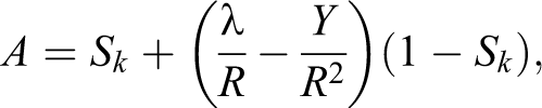
where Sk indicates the share of knowledge capital in city P. R indicates the distance from city Q, and λ indicates the spillover effects of city Q. When λ is larger, the spillover effect is greater. γ denotes the crowding effect parameters.
We assume that in the long-term equilibrium of the economy and society, capital has only two purposes: one is to maintain the economic growth and the other purpose is to compensate for the depreciation of capital. Simultaneously, we assume that the long-term growth rate (g) and depreciation rate (δ) remain unchanged. At time t, one part of material capital can still be used in
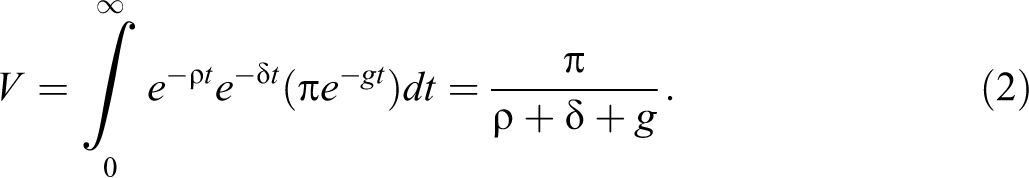
According to the goal of maximizing the profit of enterprises in the LS, the unit company’s return is
According to the above assumptions, the newly created capital has only two purposes: one is to compensate for the depreciation of capital, that is,
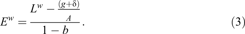
After analyzing consumer equilibrium and producer equilibrium, when the entire capital market is in equilibrium, the economy and society as a whole reaches a complete equilibrium (Walras equilibrium). Tobin’s q theory refers to the ratio of the market value of capital to its replacement cost. When

By including the distance parameter A into equation (4), we obtain

Labor productivity can be expressed as
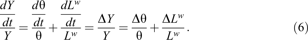
The economic growth rate is
From equation (7), the economic growth rate can be expressed as the growth rate of labor productivity and the growth rate of labor. This article defines the maximum value of labor productivity as the optimal economic efficiency of the city. At the same time, to solve for labor productivity, the integral of equation(7) on time t and the solution can be obtained as follows:

where C is a constant in equation (9); by taking the first partial derivative of equation (9) with respect to distance R and making the partial derivative zero, we obtain
Through the above analysis, by considering the combined effects of the spillover effects and the crowding effects, urban economic efficiency will increase with the distance between cities, and then it will decrease. The inverted U-shaped trend will reach the maximum at the distance
The Geometrical Description of the Optimal Intercity Distance
To describe the existence of the optimal intercity distance more intuitively, we analyze it graphically. Figure 1 reflects the trend of the spillover effects and crowding effects with the intercity distance. These two effects are mainly reflected in the economic growth rate, where the horizontal axis represents the intercity distance and the vertical axis represents the economic growth rate. The spillover effects have a positive impact on the economic growth rate, while the crowding effects have a negative impact. Therefore, the dotted line in the upper half of the horizontal axis represents the centripetal force curve of the spillover effects as a function of distance, and the dotted line below the horizontal axis indicates that the crowding effects vary with distance. The solid line is the combined force of the two forces plus the total force, which is the difference between the centripetal force and the centrifugal force and represents the net value of the spillover effect. Figure 2 reflects the trend of labor productivity with the intercity distance, where the horizontal axis represents the intercity distance and the vertical axis represents labor productivity. From the results of equation (9), we see that labor productivity is always greater than zero. When we solve the first derivative of the distance between equations (5) and (9) and let the derivative be 0, the maximum points of the economic growth rate and labor productivity are obtained at
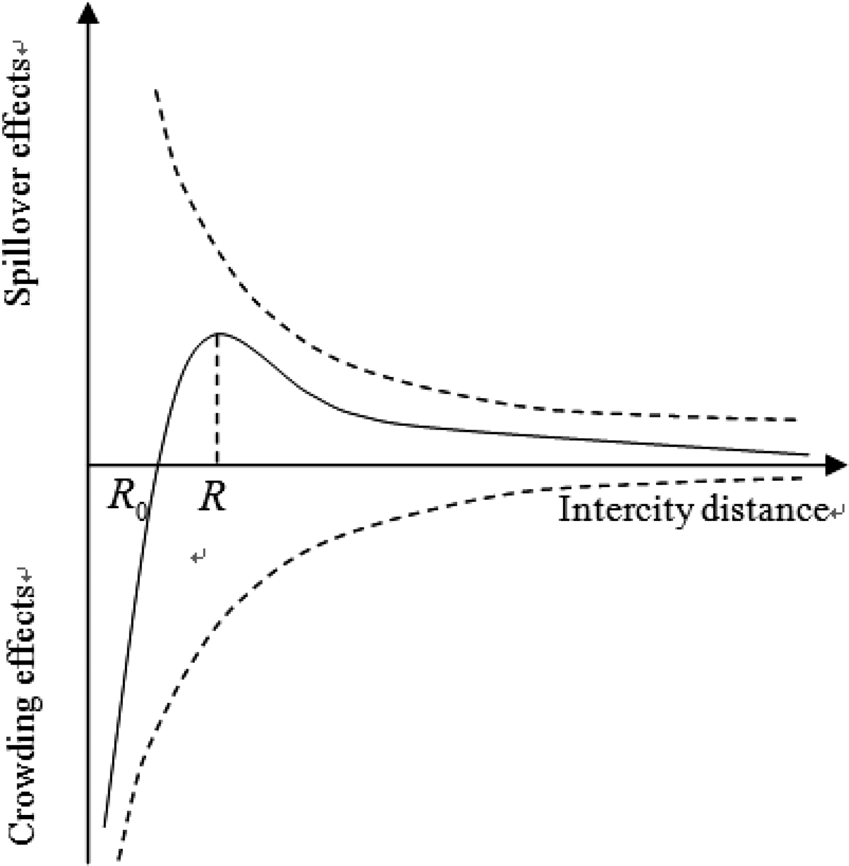
Diagram of the economic growth rate.
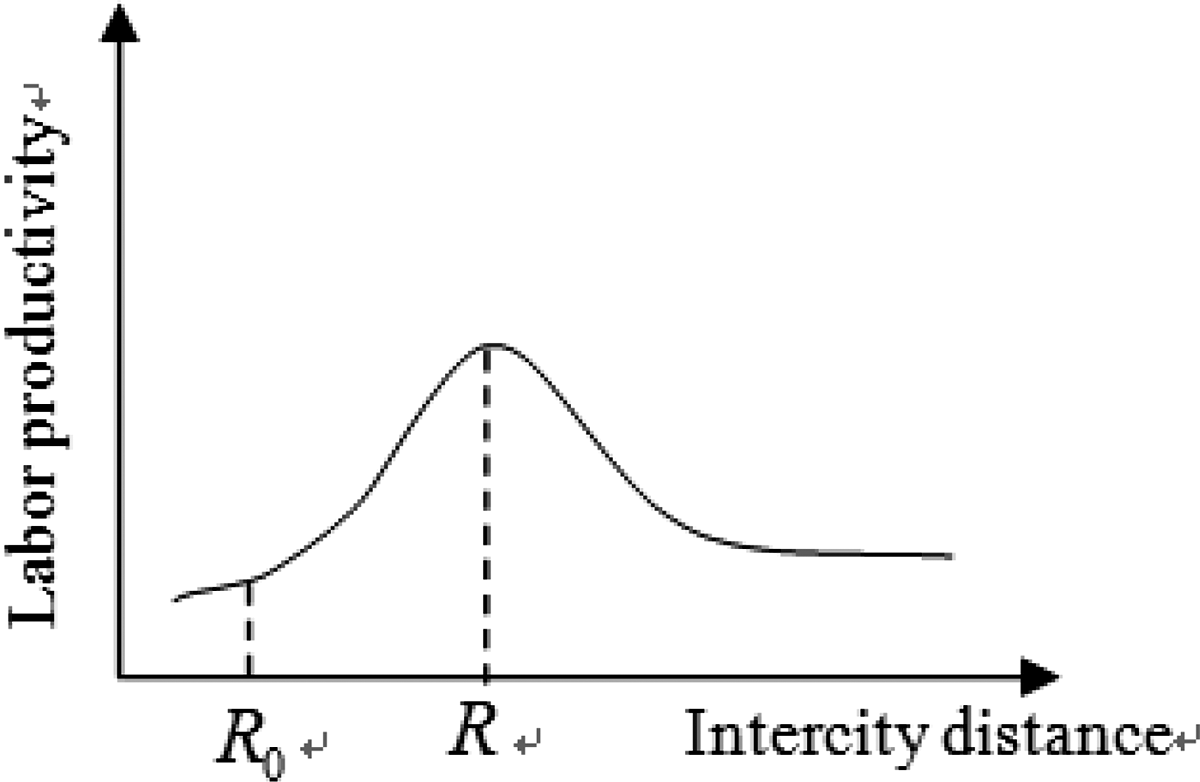
Diagram of the labor productivity.
Figure 1 reveals that if the intercity distance is very close, then the centrifugal force is much larger than the centripetal force, and the resultant force of the two forces is the net centrifugal force. As the distance increases, both the centrifugal force and the centripetal force will decrease, but because the centrifugal force drops faster, based on experience, distance-related congestion costs such as land prices and housing prices will decrease rapidly with the distance. Moreover, the division of labor between cities will always exist at a certain distance R0, and the centrifugal force is just equal to the centripetal force; as the positive and negative forces between cities are exactly equal, all the benefits of knowledge spillover are offset by rising production costs, the economic growth rate is just zero, and labor productivity is still very low. On the left side of R0, the intercity distance is too close, which intensifies competition, and cities will compete for resources, including competing for the needs of consumers, and form a siphon effect and a “Black Under the Light” effect; that is, the dominant city absorbs resources and develops, whereas the subordinate city stagnates or even declines. With the further expansion of the intercity distance, the centripetal force gradually begins to play a major role, and the combined force gradually appears as a net centripetal force. Cities have begun to enjoy the benefits of the spillover effects, urban economies have begun to grow, and labor productivity has increased as the economy has grown. When the distance reaches R, the difference between the centripetal force and the centrifugal force is the largest, the resultant force reaches the highest point, and the economic growth rate of the city reaches its maximum; at this time, labor productivity is also at its maximum. At this optimal distance, the city can maximize the enjoyment of the benefits of knowledge spillovers and avoid decreased economic efficiency caused by over constrained costs and congestion costs. Thereafter, when the distance exceeds R, although there remains a centripetal force, the impact on the economic efficiency of the city is far from the optimal state when the distance is R. Therefore, there is an optimal intercity distance, and at this distance, the economic efficiency of the city is maximized.
Econometric Framework
The Econometrics Model
According to the above theoretical derivation of economic efficiency, it can be seen from equation (9) that the economic efficiency of a city is determined by the capital stock, the number of laborers, intercity distance, the spillover effects, and the crowding effects. Intercity distance, the spillover effects, the crowding effects, and capital stock are the key factors determining the economic efficiency of the city. To better estimate the optimal intercity distance, some control variables, such as city size and urban transportation facilities construction level, must added to eliminate the impact of other variables on urban economic efficiency. At the same time, considering the possible heteroscedasticity between the data of different variables, this article takes the logarithm of all variables, and the measurement model is designed as follows:

where θ is the explanatory variable, indicating the economic efficiency of the city measured by urban labor productivity, Distance is the intercity distance,
Data Source and Sample Analysis
Our empirical data mainly come from two aspects, and one aspect involves the measurement of intercity distance. We believe that the intercity distance refers to the distance between the cities in the city center. In general, this distance includes the straight-line distance, highway distance, railway distance, and so on. However, the straight-line distance cannot reflect the accessibility between cities based on terrain. Moreover, considering that some cities’ train stations are not in the city center, the railway distance will vary greatly with the appearance of high-speed railways. Combined with Guo and He, (2012) and Chen and Ma’s (2017) research, this article studies the use of the highway distance. In general, the nearest city has the greatest impact on a city. Therefore, to reduce the difficulty of data collection, the average distance of the city from the city’s jurisdiction to the surrounding cities and municipalities is used to measure the average distance of the city, which reflects the intercity distance. The specific approach is to calculate the intercity distance by using Google Maps (see http://lcb.sxwl.com.cn/).
The second type of data is from the National Bureau of Statistics. Because of China’s urban-planning needs, urban areas are appearing and merging, which results in statistics for 291 cities in China. To ensure data completeness and stability, we select 2009–2015 and 285 prefecture-level cities as our research samples. The data collection includes economic efficiency, the crowding effects, the spillover effects, capital stock, city size, and the transportation infrastructure construction level. Economic efficiency is replaced with labor productivity.
6
The level of labor productivity can be expressed by the number of products produced in a unit of time by the same laborer. When more products are produced, the labor productivity is higher. According to Fujita, Krugman, and Venables (1999), the crowding effect is mainly determined by the “Market Competition Effect.” With an increasing number of people and enterprises, market competition becomes increasingly intense. Therefore, this article uses population density and urban enterprise density to measure the urban crowding effect: crowding effects = 0.5 × population density + 0.5 × enterprise density. However, since the scales of these two variables are different, to maintain the consistency of the quantization standards between the data, we first standardize the original data. The spillover effects mainly include knowledge spillover and the technology spillover effects, which is usually expressed by research and development investment. The urban scale and the level of transportation infrastructure construction are expressed by the number of people in the municipal districts and the city freight volume, respectively. Considering the estimation of capital stock and Zhang, Wu, and Zhang (2004), who sets the depreciation rate as
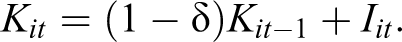
Summary Statistics.
Note: There are 1,995 observations for each variable. The data come from the China Urban Statistical Yearbook.
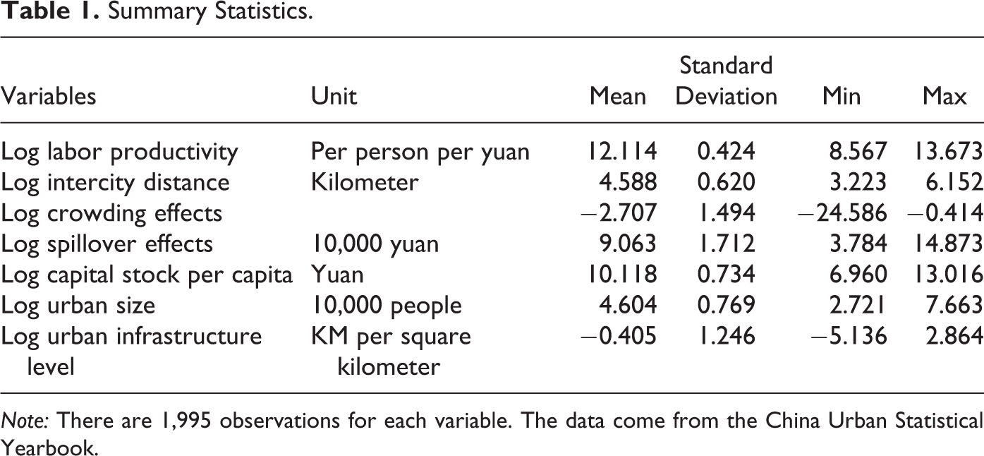
In view of the above analysis of the optimal intercity distance, some abnormal points are removed, and a scatter plot of the intercity distance and urban labor productivity is drawn. Among them, the horizontal axis represents the natural logarithmic value of the intercity distance, and the vertical axis represents the natural logarithmic value of labor productivity. Each data point in Figure 3 represents the correspondences between labor productivity and intercity distance in a city. As seen by the fitting curve (Regression software programs graph the sample points and give the curve that best fits the points), it reveals that there is an inverted U-shaped curve between urban labor productivity and the urban distance. Therefore, in the urban spatial layout, there must be an optimal distance to achieve the greatest economic efficiency between cities.
Scatter plot of labor productivity and the intercity distance.
Empirical Results and Discussions
Benchmark Analysis
Based on the above analysis, a general quantitative regression model is first provided, where model 1 is a regression model that does not consider the square term of the intercity distance and model 2 is a regression model that adds the squared term of the intercity distance to the standard deviations of heteroscedasticity. Model 3 is a random effects model. Considering that our variables include the intercity distance and the square value of the intercity distance, two explanation variables may be multicollinear. We found through the variance inflation factor (VIF) tests that the values of these two indicators are much larger than 10, which is consistent with our expectations; therefore, we use the correction method to remove the mean to obtain the result of model 4. We found that by removing the mean of the intercity distance and the square value of the intercity distance, the VIF of all variables is approximately 1. Thus far, we can conclude that none of the variables have collinearity.
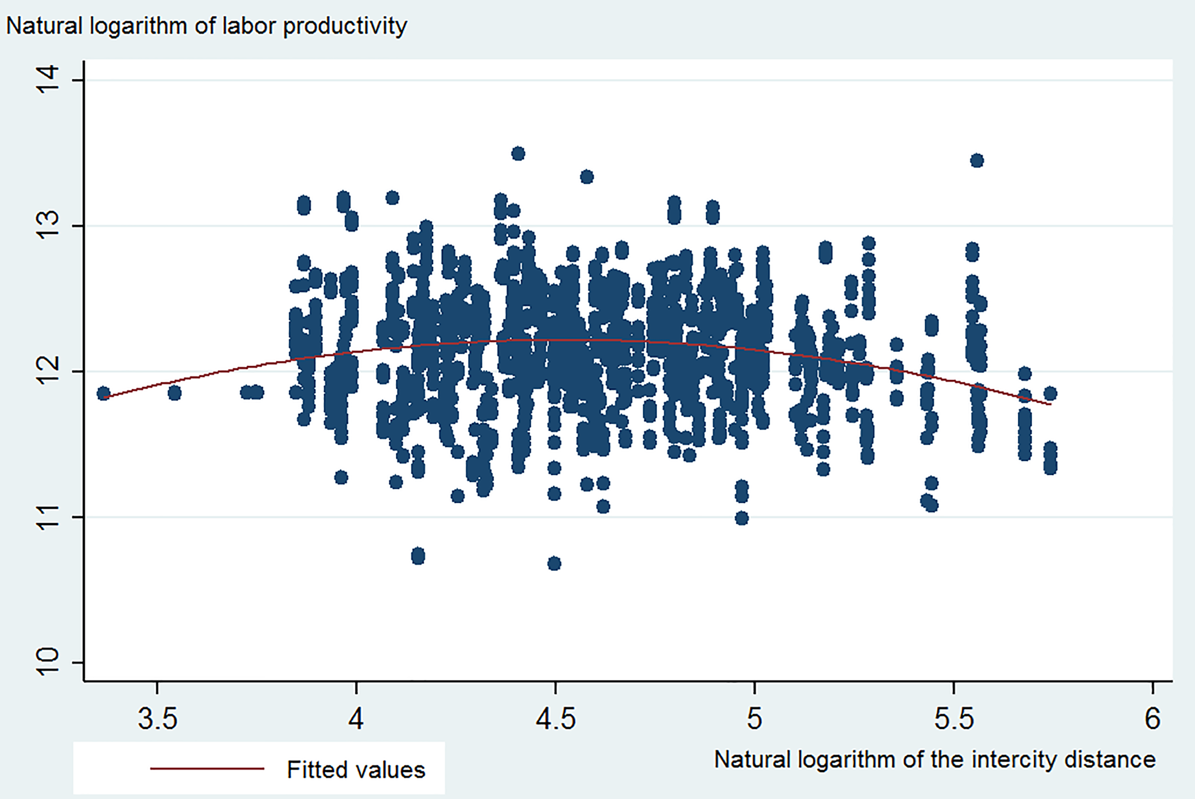
Table 2 shows the regression results for different models, and the following conclusions can be drawn. A comparison of models 1 and 2 indicates that the relationship between urban labor productivity and the intercity distance is not a simple linear relationship but is related to the square of the intercity distance. It can be seen from the significance level and R2 that the random effects estimator is a more reasonable research method. Further study of the coefficients of the distance term and the square of the distance can be found: the coefficient of one item is positive, and the square coefficient is negative. According to a simple mathematical analysis, the intercity distance and labor productivity of the city show an inverted U-shaped curve. For the results of model 3, the logarithm is processed, and the optimum distance between cities is 110 kilometer nationwide. Model 4 is the result of removing the average of the core explanatory variables. By restoring the results, we found that the optimal intercity distance is not much different from the results of model 3. Therefore, we obtain the optimal intercity distance without considering the spatial correlation. The optimal intercity distance is 110 kilometer. Simultaneously, the coefficient of the spillover effect is positive, while the coefficient of the crowding effect is negative, which is consistent with the conclusions of Conley and Ligon (2002) and Henderson (1986).
Benchmark Estimation Results.
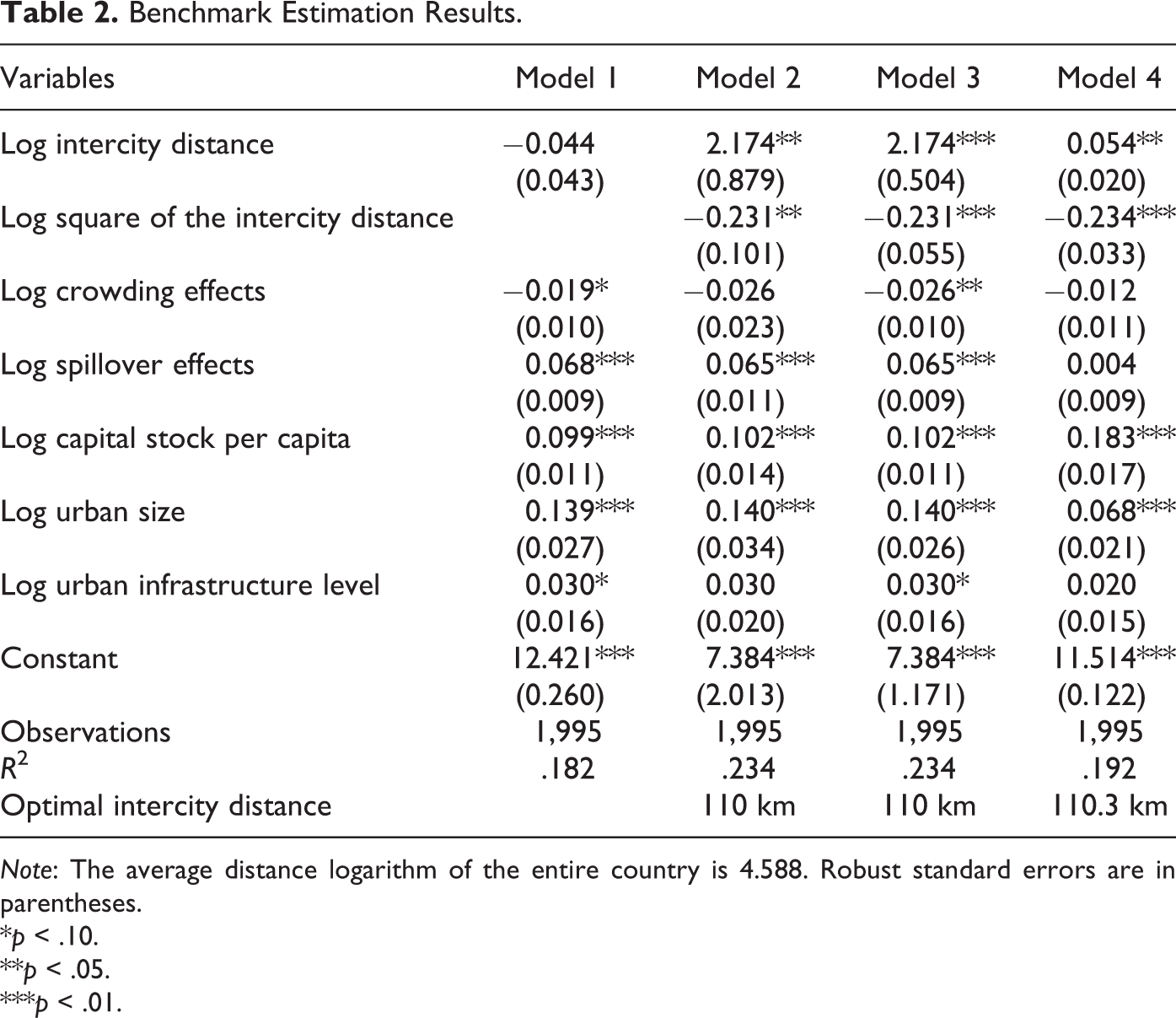
Note: The average distance logarithm of the entire country is 4.588. Robust standard errors are in parentheses.
*p < .10.
**p < .05.
***p < .01.
According to the characteristics of China’s topographic distribution, the eastern terrain is relatively low, while the western terrain is on a plateau. Therefore, topography causes the generally large intercity distances in the west and the small intercity distances in the eastern and central regions; 7 thus, the optimal intercity distance cannot be the same. This article excludes the impact of the northeastern region on the layout of the eastern cities 8 and analyzes the optimal scale of different regions under the consideration of the geographical location factors. Combined with some methods of regional division, this article divides China into eastern, central, western and northeastern regions. The prefecture-level cities are divided into four regions according to their respective states.
Table 3 presents the results for different regions, except for the central region. The core explanatory variables of the other three regions are significant at the 5 percent level, which indicates that it is reasonable to add the squared term of the distance to the measurement model. By restoring the data of the core explanatory variables, we obtain an optimal intercity distance of 91 kilometer in the eastern region, 115 kilometer in the western region, and 101 kilometer in the northeastern region. Thus, the eastern region is mostly in the plains, where there is overpopulation and the industries are intensive. The intercity distance is not too large compared with the average optimal intercity distance in the country. The western region is mostly plateau, with a lower population and a lower industrial density. The density is relatively low, and the intercity distance should not be very small. However, the central region is not significant. The traditional panel model has defects that are relevant to this article’s investigation. It does not consider the spatial correlation of the geographic regions, and it is therefore difficult for the traditional panel model to accurately measure the spatial differences of this region. This article constructs a spatial econometric model and studies it from the perspective of geographic space.
Regression Results by Region.
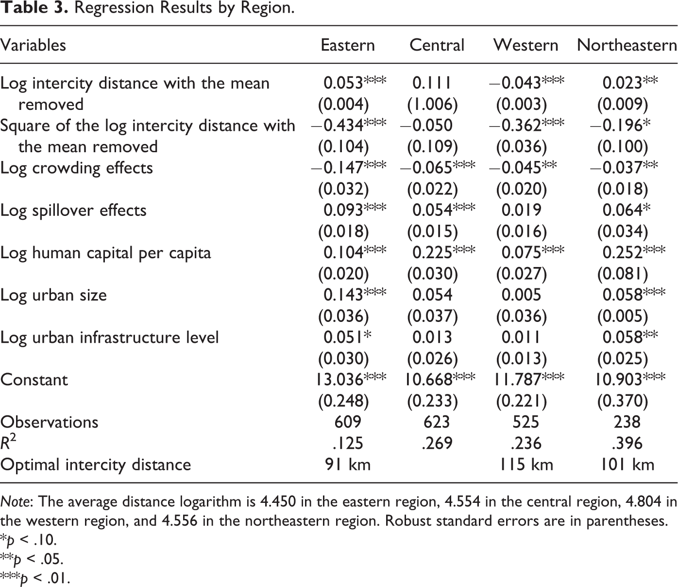
Note: The average distance logarithm is 4.450 in the eastern region, 4.554 in the central region, 4.804 in the western region, and 4.556 in the northeastern region. Robust standard errors are in parentheses.
*p < .10.
**p < .05.
***p < .01.
Spatial Econometric Model
The First Law of Geography tells us that spatial correlation is a nonnegligible factor in the study of regional economic issues. In the previous part of the study, there is no doubt that the spatial correlation between cities is not fully considered. Therefore, to estimate the optimal intercity distance more accurately, this article constructs and analyzes a spatial econometric model of urban labor productivity, and the model is as follows:

Equation (11) is a general space panel model. Since the parameters are not the same, the model will usually be different as follows: if
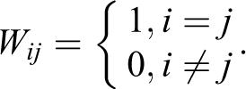
There are usually two methods of setting the weight matrix: one is to construct a 0–1 matrix (adjacent to 1 and not adjacent to 0) based on whether the geographical locations are adjacent; the other method is based on the reciprocal value of the distance between cities. The reciprocal value is used as the weight matrix. Considering that the core explanatory variables of this article are the distance between cities, to avoid interaction between the data, the first method is chosen in this article, and the weight matrix is set as follows:
Through the spatial weight matrix, the global Moran’s and local Moran’s indexes of urban economic efficiency are obtained. The global Moran index can reflect that the urban economic efficiency and the intercity distance in China have a significant spatial autocorrelation as a whole. The local Moran index can reflect the spatial characteristics of China’s urban economic efficiency and the intercity distance.
Figure 4 shows the local Moran’s index scatter plot of the labor productivity of 285 prefecture-level cities in 2009 and 2015. The first quadrant represents the spatial connection form in which the regional unit of high observation value is surrounded by the same high-valued region. The second quadrant represents the spatial connection form of the regional unit of low observation value surrounded by the high-valued region. The third quadrant represents the form of spatial association in which the low-valued regional unit is surrounded by the same low-valued region. The fourth quadrant represents the spatial association of the high-valued regional unit surrounded by the low-valued region. The first and third quadrants have strong spatial dependence, while the second and fourth quadrants have more intense spatial heterogeneity. Figure 4 also shows that most of the cities are located in the first and third quadrants, which indicates that the spatial correlation among cities is strong. Further analysis finds that low-value clustered cities migrate to high-value cluster cities as time increases, and most of the first quadrant is still in the eastern coastal cities and some economically developed cities. Because the intercity distance is very close and industry is intensive in the eastern region, the spillover effect on neighboring cities is obvious, and it is more likely that high labor productivity cities will drive the development of neighboring cities together. In contrast, most of the third quadrant is in the central and western remote areas. Compared with the average distance of cities across the country, some cities in the central and western regions have greater distances, fewer people, and less industrial density. The spillover effect is not significant, and it is difficult to develop through knowledge spillovers from neighboring cities.
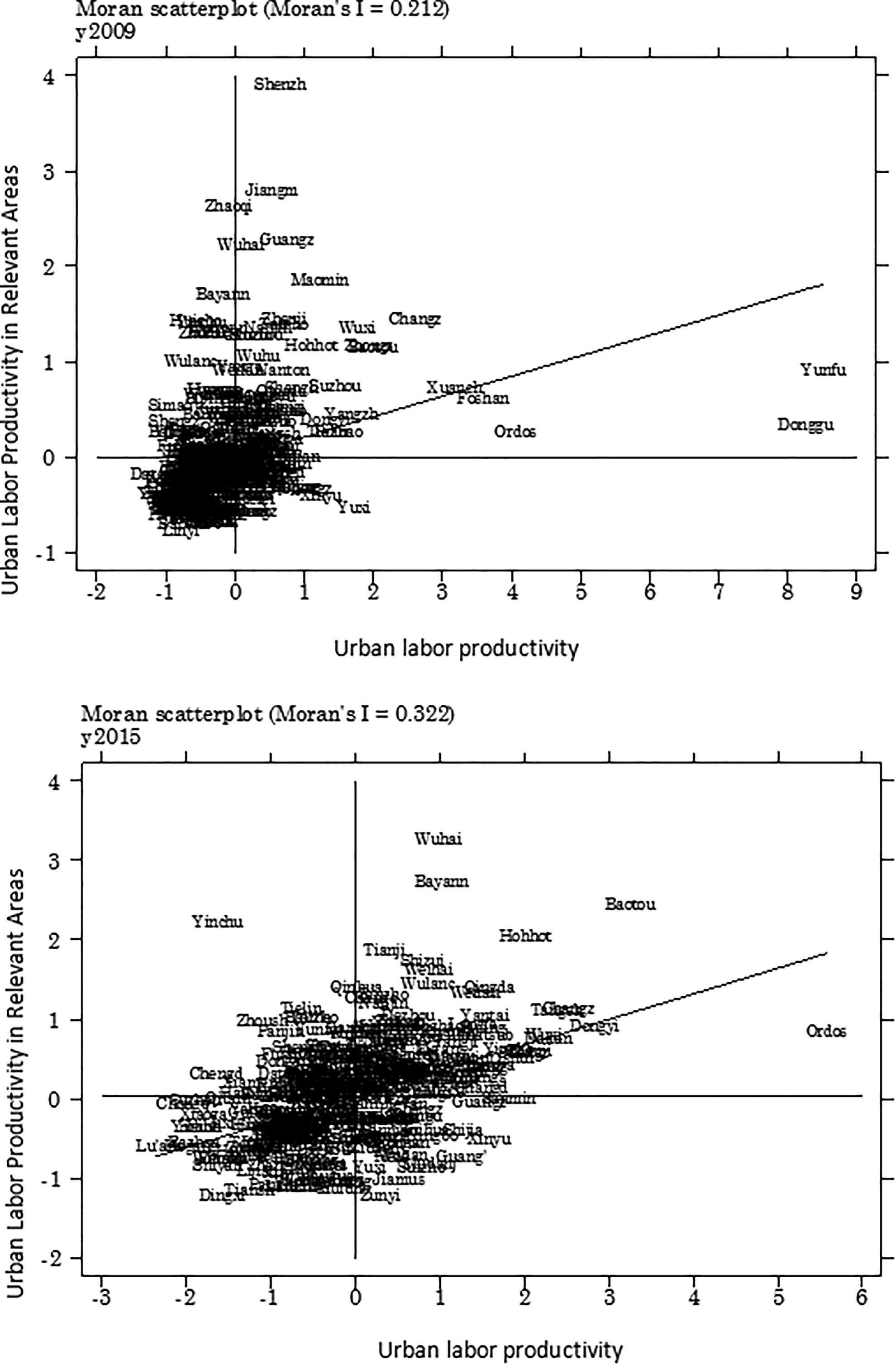
Scatter plot of the Moran’s index of urban labor productivity in 2009 and 2015.
Results of the Spatial Econometric Models
Since the intercity distance is a variable that does not change over time, it cannot be regressed by fixed effects, and the result of the Hausman test cannot be obtained. Therefore, this article gives panel regression results for three different spatial econometric models based on random effects: model 4 is an SAR, model 5 is an SEM, and model 6 is an SDM.
Table 4 presents the estimated results under different measurement models. After adding the spatial interaction factors,
Regression Results of Various Spatial Econometric Models.
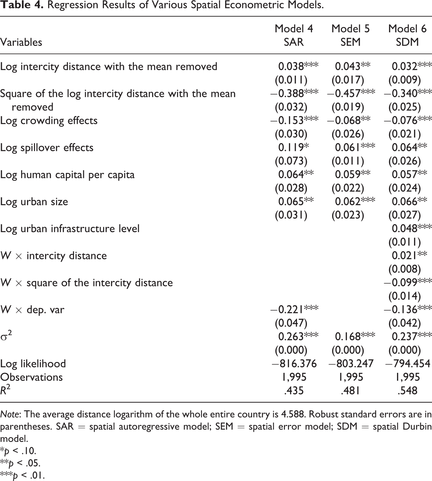
Note: The average distance logarithm of the whole entire country is 4.588. Robust standard errors are in parentheses. SAR = spatial autoregressive model; SEM = spatial error model; SDM = spatial Durbin model.
*p < .10.
**p < .05.
***p < .01.
Table 5 presents some evidence for that regional hierarchies are important for optimal distance. The negative coefficient of the square term of the distance between cities indicates that even if they are divided into different regions, the labor productivity of the city presents an inverted U-shaped trend. It can be further calculated by simple mathematical analysis that the optimal intercity distance in the eastern region is 95 kilometer, the optimal intercity distance in the central region is 105 kilometer, the optimal intercity distance in the western region is 114 kilometer, and the optimal intercity distance in the northeastern region is 103 kilometer. Overall, from east to west, the optimal intercity distance increases. By comparing the results in Tables 3 and 5, when considering urban interaction, the optimal urban distance in the eastern region is slightly larger than the optimal intercity distance without considering the spatial correlation, and it is slightly smaller than the optimal urban distance in the western region. From this conclusion, we find the role of “centripetal force” and “centrifugal force.” Because of its intensive industry and large population, the eastern region has formed urban agglomerations such as the Bohai Sea, the Yangtze River Delta, and the Pearl River Delta. Because the intercity distance is very close and centrifugal force plays a dominant role, the crowding effect deviates from the optimal state of urban development in the eastern region. Similarly, for the western region, centripetal force plays a role because of the high topography, high transportation costs, and relatively long intercity distances. This finding also indirectly verifies the impact of the intercity distance on urban economic efficiency.
Spatial Dubin Model Regression Results for Eastern, Central, Western, and Northeastern China.
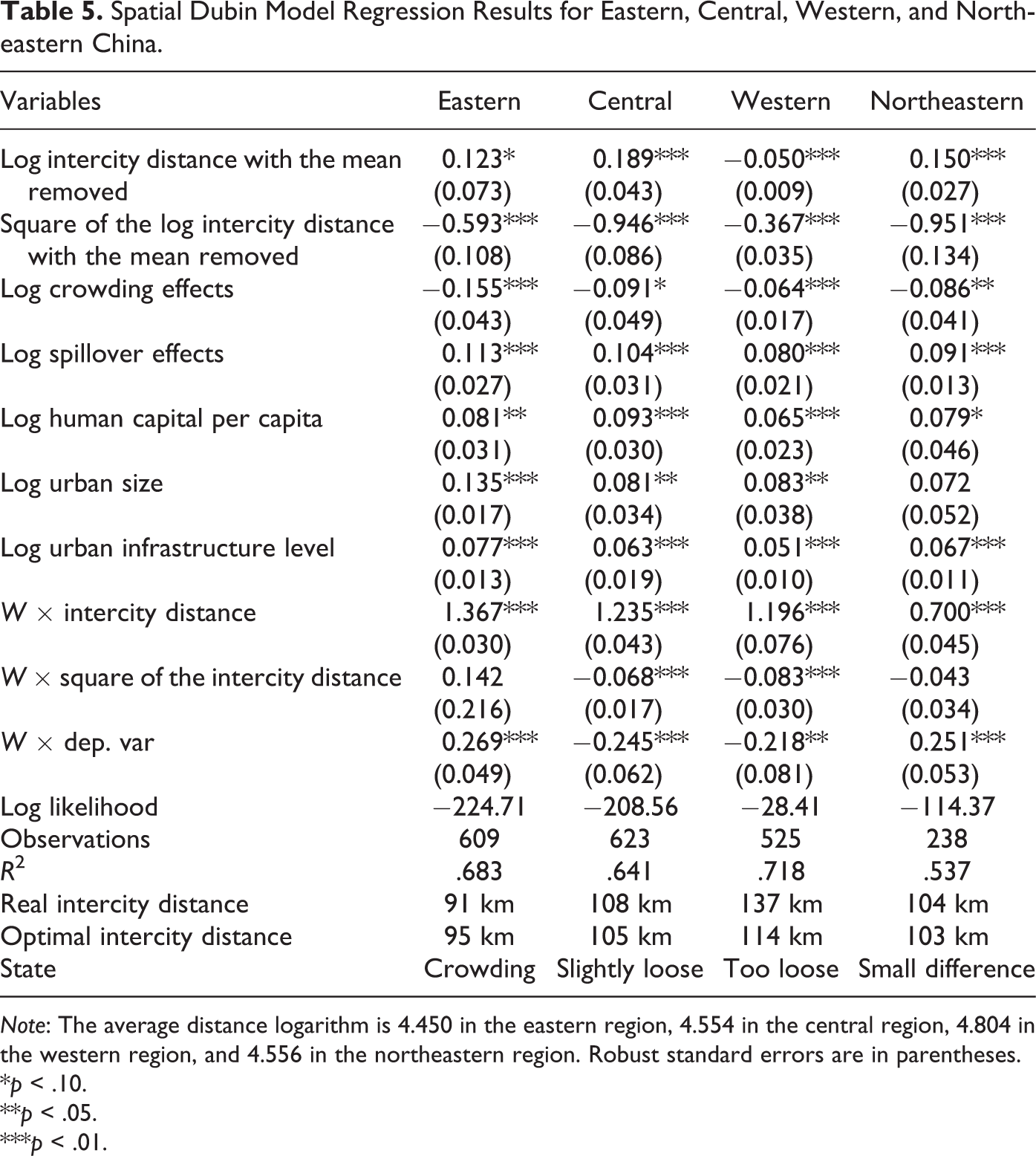
Note: The average distance logarithm is 4.450 in the eastern region, 4.554 in the central region, 4.804 in the western region, and 4.556 in the northeastern region. Robust standard errors are in parentheses.
*p < .10.
**p < .05.
***p < .01.
Urban Regional Planning Analysis
There are still many prefecture-level cities in China with large administrative areas and large populations. The range of urban radiation is limited (Xu, Jiao, and Zhu 2013), their per capita gross domestic product (GDP) is much lower than the other prefecture-level cities adjacent to them, and some prefecture-level cities’ GDP is at a lower level. 9 For example, Ganzhou and Nanyang are located in central China. The area of Ganzhou City is 39,380 square kilometers, and the population is 9.75 million. The area of Nanyang City is 26,600 square kilometers, and the population is 8.64 million, which is standard for a prefecture-level city. We refer to Liu, Derudder, and Wu (2016) to describe the distribution of prefecture-level cities in China. According to the optimal distance between cities estimated by the above analysis, we obtain an optimal urban distance of 105 kilometer in the central region. On the basis of the urban radiation circle, in the surrounding areas of Nanyang and Ganzhou, the urban distribution is too sparse, it means that there are still some “blank areas.” Combined with the optimal distance of the city, the economic base, and terrain of each county-level city, we propose to add Ruijin and Xixia as prefecture-level cities. This is also consistent with Liu’s view that areas with higher population bases are more suitable for developing urban polycentricity (Liu and Wang 2016; Li and Liu 2018).
From (C) and (D) of Figure 5, the dark circle is the economic radiation range of the existing prefecture-level city and the light circle is the radiation range of the newly added prefecture-level city. Before the addition of prefecture-level cities, there were urban blank areas in Ganzhou and Nanyang because of the large area involved, and it was difficult to cover the entire administrative area with the radius of urban radiation. Some areas could not enjoy the benefits of the urban spillover effects, which decreased the average level of urban economic efficiency. By adding Ruijin and Xixia as prefecture-level cities, the urban distance of each city is optimal, and the emergence of new cities has greatly reduced the number of urban blank areas. The newly added cities fill the urban gaps in these areas and play a leading role in poverty-stricken areas, which is of great significance for the planning and layout of Chinese cities.
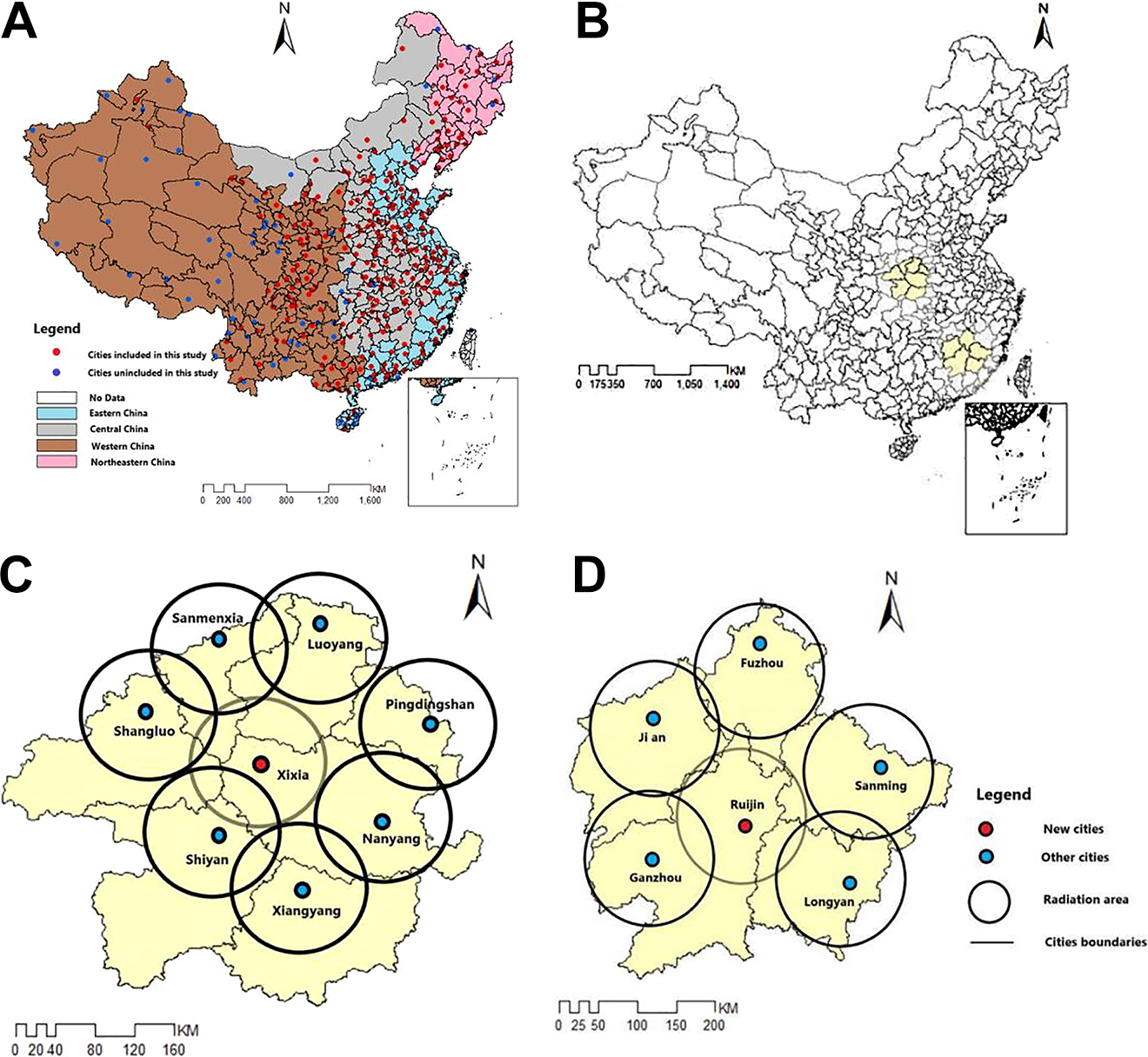
(A) Distribution of prefecture-level cities in China. (B) The location of Ganzhou, Nanyang, and surrounding cities in China. (C) The map after the new addition of Xixia City in Nanyang. (D) The map after the new addition of Ruijin City in Ganzhou.
Concluding Remarks and Policy Implications
Based on the “centripetal force” and “centrifugal force” of the intermolecular distance model in physics, this article establishes a mathematical model to analyze the influence of the distribution of cities on urban labor productivity. We also incorporate the crowding parameter into the LS model and demonstrate the existence of the optimal intercity distance. With an increase in the distance between cities, the urban labor productivity shows an inverted U-shaped trend. According to data from the prefecture-level cities in China, the average optimal distance between cities in China is estimated to be approximately 103 kilometers. From the eastern region to the central region to the western region, the optimal intercity distance among cities increases in turn. Judging from the deviation between the actual average distance and the optimal average distance in each region, the cities in the eastern region are crowded, and the cities in the central and western regions are sparse.
Geography also seems to affect economic policy choices (Gallup, Sachs, and Mellinger 1999). For the central and western regions of China, where the administrative areas are large and have a large population (such as Ganzhou City and Nanyang City), there is serious boundary poverty. Appropriately increasing the number of prefecture-level cities and increasing industrial density through industrial transfer and development not only will help to improve the urban economic efficiency in the central and western regions but will also reduce congestion in cities in the eastern region. This approach takes full advantage of the radiation effects on rural areas and achieves the goal of an affluent society.
Footnotes
Appendix
As discussed in section “Modeling the Optimal Intercity Distance” of the main text, the derivation of the profit function in the LS is derived from the capital creation model. The derivation process is as follows.
Suppose an enterprise in P city has a sales volume of c and a sales price of p in the local market, while a sales volume of Q in another city is
By maximizing the utility of consumers, we can get that the consumption of P city is
From the maximization of consumer utility, we can conclude that the P city industrial price is:
The number of enterprises in the north is represented by n, and the number of enterprises in the south is represented by
Q city industrial price is:
Thus,
Acknowledgments
The authors would like to thank the editor of the journal and the three anonymous referees for their comments and detailed suggestions, all of which were valuable and very helpful for revising and improving the quality of our article. They would also thank Vernon Henderson, Yilun Tong, and many seminar participants for their useful comments. Specifically, the authors thank Weiyong Zou for his research assistance.
Declaration of Conflicting Interests
The author(s) declared no potential conflicts of interest with respect to the research, authorship, and/or publication of this article.
Funding
The author(s) disclosed receipt of the following financial support for the research, authorship, and/or publication of this article: This work was supported by the key research projects of philosophy and social science of Chinese Ministry of Education (11JZD018) and the Graduate Research Innovation Project of Hunan Province in 2017 (CX2017B579).