Home Is Where the Internet Is? High-speed Internet’s Impact on Rural Housing Values

Abstract

The deployment of faster household Internet speeds enables new opportunities for entertainment, social interaction, and personal development, and many consider such access an essential component of everyday life. However, rural residents face lower availability, slower speeds and limited provider options, putting them at a disadvantage when compared to their urban counterparts. Connected rural households, especially those with higher speeds, may experience a premium on their home value. Data from the National Broadband Map, the Federal Communications Commission, and over 2,700 housing transactions from June 2011 to June 2017 are used to examine the impact of broadband availability on housing values in two rural Oklahoma counties via a hedonic price model. The results find no support for the existence of a broadband premium, and stress that differences across counties are crucial in assessing rural housing prices.

Keywords

broadband housing values rural counties hedonic

Telephone lines revolutionized communication. The National Highway System revolutionized travel. The Internet revolutionized how people go about their everyday lives. High-speed Internet, or broadband, has the ability to connect people across time and space.¹ Broadband—especially in rural areas—opens doors to countless opportunities, including advances in telemedicine, educational resources, and web engine searches leading to news and job opportunities. However, Internet access and availability in rural areas has always lagged behind their urban counterparts. This continues to be the case, with only 73.6 percent of rural residents (compared to 98.3 percent of urban) having access to the current definition of fixed terrestrial broadband as of December 2017 (Federal Communications Commission [FCC] 2019).²

Residential, high-speed Internet access gives consumers the capability to stream music, watch movies, interact socially, become civically engaged, and perform a variety of everyday tasks from the comfort of their own homes. A recent survey reported that 77 percent of Americans say they go online daily, and 26 percent report going online “almost constantly” (Perrin and Jiang 2018). Not surprisingly, those living in urban areas are twice as likely to go online almost constantly compared to rural residents (Perrin and Jiang 2018). There is strong evidence that broadband connections have changed the way we obtain information and entertainment, but 58 percent of rural residents believe access to high-speed Internet is a problem in their area (Anderson 2018).

The lagging broadband availability in rural areas is an important piece to the “digital divide” in broadband adoption rates (Whitacre, Strover, and Gallardo 2015). Urban residents can often choose between Internet providers, with 44 percent having access to more than one provider of wired broadband such as cable, Digital Subscriber Lines, or fiber (FCC 2016, 2019). ³ Comparatively, only 13 percent of rural residents have access to more than one provider of wired broadband (FCC 2016). Internet Service Providers (ISPs) typically incur higher installation costs for deploying high-speed Internet to rural areas due to a more sparse population and more rugged terrain. This cost often is transferred to the consumer, leading to a “rural penalty” for those living in remote areas (Malecki 2003). As one example, after buying land and building a house, a Wisconsin man was told by the local ISP they would only offer service to his location if he paid $117,000 to cover the cost of extending their network to his location (Brodkin 2015a).

Anecdotally, some rural residents are willing to pay a premium for a faster, reliable Internet connection. After struggling with slow speeds, a farmer in Nebraska was willing to pay the nearly $42,000 requested by the ISP to subsidize construction for a fiber line, noting, “…it is a one-time investment that will enhance my quality of life and property value significantly” (Brodkin 2015b). Real estate agents in Vermont note the difficulty associated with selling homes without broadband, and some argue that depending on the property’s location, “…broadband access can make or break the deal” (Picard 2016). These examples point to an increased demand for high-speed broadband services and suggest consumers place a value on readily available Internet access. However, little empirical work has been done on this topic, especially pertaining to rural households.

Rural areas with access to broadband are linked to increased economic activity and growth, including positively impacting firm location decisions (Kim and Orazem 2017), household income growth (Whitacre, Gallardo, and Strover 2014a, 2014b), and domestic in-migration (Mahasuweerachai, Whitacre, and Shideler 2010). While rural America has seen a recent increase in overall population, an aging baby boomer generation coupled with the opioid epidemic has caused a decline in the natural change (births minus deaths). As natural change is projected to continue falling (Cromartie 2018), future population growth in rural America will increasingly rely on in-migration. With today’s youth growing up in an era of touch screens and constant connectivity, the availability of high-speed broadband infrustructure is likely high on the list of must-have amenities for new homeowners. However, an important question to answer is: do rural households where broadband is available garner a premium? If so, subsequent growth in broadband infrastructure could result in increased property tax collections, potentially generating additional revenue for rural areas that have struggled financially.

This article aims to examine the relationship between high-speed broadband availability and housing values, specifically in rural America. Broadband download speed data from the National Broadband Map (NBM) and the Federal Communications Commission (FCC), along with housing transaction values for two Oklahoma counties, are collected for 2011–2017. Using a spatial hedonic framework that controls for home characteristics, we estimate the contribution of broadband availability on a rural house’s sale price. Our findings vary by county but generally offer no support for the existence of a broadband premium.

Literature Review

Several studies have empirically addressed the consumer benefits associated with broadband Internet, finding high consumer surplus values (Dutz, Orszag, and Willig 2009; Goolsbee and Klenow 2006). Rosston, Savage, and Waldman (2010) use choice experiments to estimate consumer utility from Internet access and found that consumer surplus per household increased from $6.49 to $39.44 between 2003 and 2010. Nevo, Turner, and Williams (2016) estimate consumer surplus for broadband access to be $160–$236 per month, assuming a $70–$100 monthly fee. Czernich et al. (2011) find that a 10 percentage point increase in broadband penetration resulted in a one percentage point increase in Gross Domestic Product (GDP) per capita for Organization for Economic Cooperation and Development (OECD) countries between 1996 and 2007.

Spillover effects of broadband have extended to many aspects of personal and community development (Devaraj et al. 2017). A large body of evidence has investigated the impacts of broadband deployment on a variety of social and economic outcomes. Overall, broadband availability is positively associated with a host of economic growth measures (Holt and Jamison 2009). Specifically, positive relationships have been found between broadband availability and employment rates (Atasoy 2013; Jayakar and Park 2013), population and employment growth (Kolko 2010), and number of businesses (Gillet et al. 2006). While many positive externalities are associated with increased broadband availability, other studies have found that having faster broadband deployment has no significant impact on household incomes (Kolko 2010) or changes in unemployment rates (Jayakar and Park 2013).

Studies focusing specifically on rural areas generally find positive externalities associated with an increase in broadband technology, noting positive relationships between rural broadband access and adoption and greater economic growth (Stenberg et al. 2009). Other studies note the difference between broadband adoption and availability in rural areas. In general, increases in broadband adoption in rural areas have been linked to higher income growth, lower unemployment rates, higher median household income, and higher number of firms and overall employment levels (Whitacre, Gallardo, and Strover 2014a, 2014b). Recent studies have also found that broadband adoption, as opposed to simple availability, is more important for increased civic engagement in rural areas (Whitacre and Manlove 2016). However, in other cases higher, broadband availability in rural areas was positively linked to entrepreneurs, while high broadband adoption had a negative relationship with creative class workers (Conley and Whitacre 2016).

Broadband studies in rural areas have generally focused on larger aspects of the rural economy such as jobs and income, but questions still surround the value of broadband at the household level. This includes the impact of broadband on housing prices. Homeowners in rural areas without broadband access might experience adverse impacts on their property value. As evidenced in popular press articles, the existence of Internet access is an important factor when purchasing a home (Brodkin 2015a; Knutson 2015; Picard 2016). Does rural household broadband availability equate to more than buffer-free Netflix access—and can we put a value on it?

Hedonic models have long been used to estimate the impact of specific characteristics (i.e., presence of a garage, number of bathrooms, total square footage) in the housing market (Sheppard 1999; Baum-Snow and Kahn 2000; Liu and Hite 2013). Many of these studies have a rural focus, including research that estimates the effects of environmental amenities (Nelson 2010), water source (North and Griffin 1993), and proximity to oil facilities or hydraulic fracturing (Boxall, Chan, and McMillan 2005; Bennett and Loomis 2015; Balthrop and Hawley 2017) after controlling for traditional housing characteristics. A common factor of many of these rural-oriented hedonic papers is their inclusion of only one or two counties, possibly due to the wide variation across counties in rural America and the time-intensive nature of gathering housing transaction data. An important point brought up throughout the hedonic literature is that since housing data are spatial in nature, an econometric approach that captures any potential spatial effect is vital for avoiding omitted variable bias (Dubin 1988; Basu and Thibodeau 1998). However, some studies found that ordinary least squares (OLS) results were comparable to those from spatial econometric approaches (Geoghegan, Lynch, and Bucholtz 2003). These results form the basis of our empirical specifications.

The literature exploring the relationship between housing values and high-speed Internet connection is relatively sparse, although several studies do focus explicitly on this question. Using fifteen years (1995–2010) of property prices in England, Ahlfeldt, Koutroumpis, and Valletti (2014) suggest that upgrading to an 8 Mbps connection from dial-up increases the property value by 2.8 percent. Their cost-benefit analysis found that rural areas were problematic—namely, that the estimated benefits from a potential speed upgrade would only account for around 15 percent of the associated costs of implementing the infrastructure. This is in line with the traditional rationale for why private providers are hesitant to enter rural areas—that such investment does not provide an economic return.

Molnar, Savage, and Sicker (2015) use data from the NBM and nationwide housing transaction data to investigate whether the relationship between high-speed Internet service (specifically a fiber connection) is correlated with higher housing prices.⁴ Using 2011–2013 real estate transactions from all fifty states and DC (32 percent of all transactions occurring in California, Florida, and Ohio) and NBM data they estimate a hedonic housing price model. When controlling for speed, their estimates indicate that homes in census blocks where fiber was available had a 1.3 percent higher transaction price than similar homes in neighborhoods where fiber was not available (Molnar, Savage, and Sicker 2015). When evaluated at the median house price, this increase suggests a $5,437 increase in a home’s value if fiber Internet is available (Molnar, Savage, and Sicker 2015). The Molnar, Savage, and Sicker (2015) study examines broadband and housing values on a national level and did not emphasize rural areas which generally experience different price constraints and lower initial real estate values. We attempt to expand on their study by specifically examining rural areas and by focusing on broadband available by any fixed technology type (not just fiber).

Kashian and Zenteno (2014) focus on rural households specifically in the nonmetropolitan and tourism-dependent Door County, Wisconsin. Using a hedonic model and survey responses (n = 225) meshed with county assessor information, they found that the average value of seasonal property with Internet access increased by 2.7 percent when compared to seasonal homes without Internet access. This estimate is similar to the estimates from Molnar, Savage, and Sicker (2015) and Ahlfeldt, Koutroumpis, and Valletti (2014).

Deller and Whitacre (2019) recently address the relationship between fixed terrestrial Internet availability and housing prices for residents in remote rural counties. Using national data on nonmetropolitan counties not adjacent to metropolitan areas and a series of spatial models, they find a positive and statistically significant impact of broadband availability on housing values across five speed categories, specifically for the lower speed thresholds (Deller and Whitacre 2019). At the county level, they show that a 10 percent increase in Internet speeds is associated with an average housing value increase ranging from $230 to $661 (Deller and Whitacre 2019). These findings add to the growing literature supporting the provision of broadband in rural locations. They suggest that having high-speed Internet availability is reflected in local housing values, particularly for remote rural areas. Our study expands on this work by using a spatial hedonic framework to examine broadband’s value for an individual house using two distinct counties in a relatively rural state (Oklahoma). This hedonic approach is significantly different in nature to the aggregate county-level work performed by Deller and Whitacre (2019).

Data and Methods

This study examines the impact of high-speed broadband on rural housing prices for two rural Oklahoma counties, Woods County and Pittsburg County. Woods and Pittsburg were chosen because of their diversity (one is significantly smaller in terms of population; their topography and natural amenities are also quite different), and because they experienced significant broadband growth over the period of interest. The smaller of the two, Woods County, is located in northwestern Oklahoma (Figure 1) and has an estimated 2017 population of 9,132. The county seat, Alva, has a population of 5,167 (US Census, 2017, American Community Survey [ACS]). Woods County has a Rural–Urban Continuum Code (RUCC) of 7, indicating that it is a nonmetro county not adjacent to a metropolitan area and that it has an urban population of 2,500–19,999.⁵ Alternatively, Pittsburg County is located in the southeastern part of the state and has roughly five times more residents than Woods (2017 population estimate of 44,673). The county seat, McAlester, has a population of 18,198 (US Census, 2017, ACS). Pittsburg County has a RUCC of 5, indicating that (like Woods County) it is also a nonmetro county not adjacent to a metropolitan area but that it has an urban population of over 20,000.

Figure 1.

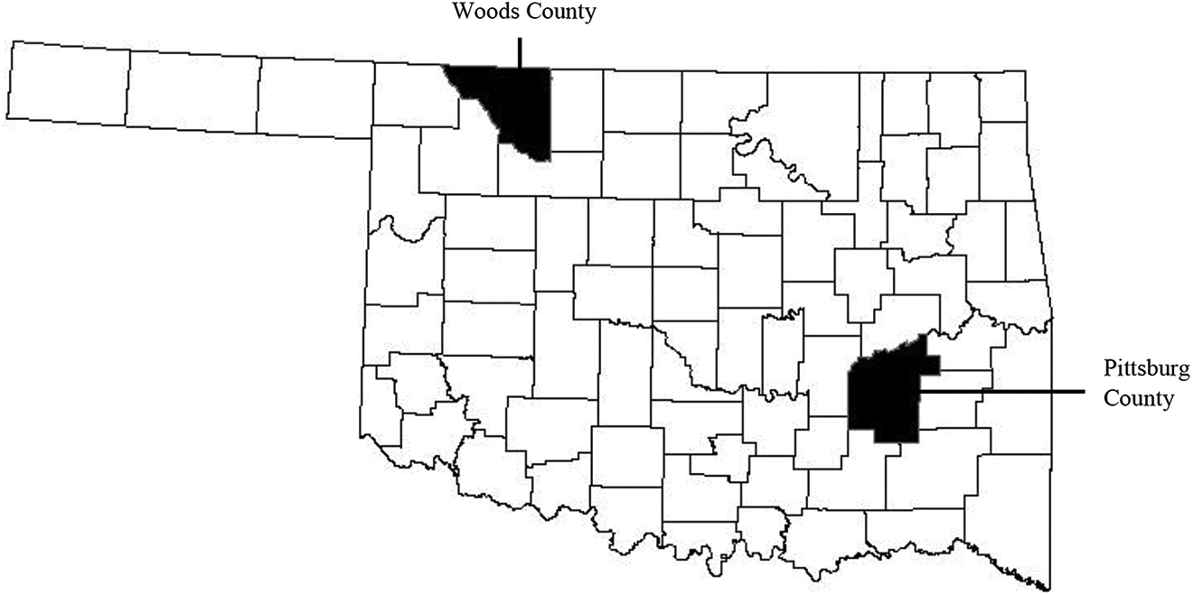
Woods and Pittsburg counties (Oklahoma).

Other factors also differentiate the two counties. According to the Natural Amenities Scale, the topography of Woods County is “irregular plains” with 0.27 percent water area.⁶ Compared to Pittsburg County, Woods County has high levels of oil and gas production. The volatility of the oil and gas industry might also have effects on the housing market, including home transaction pricing.⁷ Pittsburg County’s topography is described as “open high hills” and is comprised of 5.22 percent water—including portions of Lake Eufala, an amenity that could impact housing prices. Also important to note is that the city of McAlester in Pittsburg County is home to the state prison, which could negatively impact prices for houses in close proximity.

Woods and Pittsburg were also chosen because of their dramatic increases in broadband deployment between 2011 and 2017. Over the course of six years (June 2011–June 2017), speeds of 50 Mbps or greater went from nonexistent to available to more than 40 percent of the census blocks in Woods County. Simultaneously, the percentage of unserved census blocks went from above 20 percent to nearly zero (Table 1). Pittsburg County also saw significant improvements in broadband deployment, going from 0 percent of census blocks with coverage of 50 Mbps or greater in June 2011 to around 24 percent in June 2017 (Table 2).

Table 1.

Woods County Percentage of Census Blocks Max Download Speeds.

		Broadband Speeds
Month and Year	Unserved (%)	<4 Mbps (%)	4–10 Mbps (%)	11–25 Mbps (%)	26–50 Mbps (%)	>50 Mbps (%)
June 2011	21.98	33.66	44.36	0.00	0.00	0.00
December 2011	19.65	25.00	55.35	0.00	0.00	0.00
June 2012	24.24	24.30	51.45	0.00	0.00	0.00
December 2012	24.48	24.24	36.69	3.31	11.28	0.00
June 2013	28.26	21.16	36.45	2.97	11.16	0.00
December 2013	27.97	20.81	36.63	3.20	11.40	0.00
June 2014	26.22	22.50	28.08	11.63	11.57	0.00
December 2014	0.00	55.17	1.63	1.92	26.63	14.65
June 2015	0.00	54.24	1.98	1.92	26.45	15.41
December 2015	0.00	49.01	5.29	1.92	7.62	36.16
June 2016	0.00	0.00	54.59	1.63	7.56	36.22
December 2016	0.00	0.00	0.00	53.08	7.56	39.36
June 2017	2.27	26.80	17.79	6.22	3.60	43.31

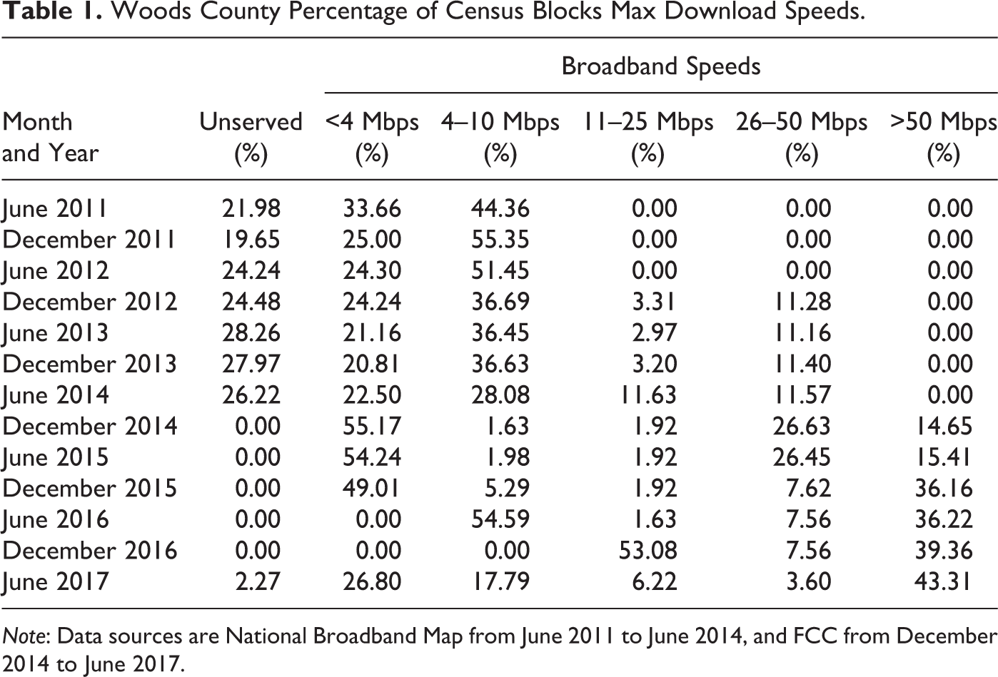
Note: Data sources are National Broadband Map from June 2011 to June 2014, and FCC from December 2014 to June 2017.

Table 2.

Pittsburg County Percentage of Census Blocks Max Download Speeds.

		Broadband Speeds
Month and Year	Unserved (%)	<4 Mbps (%)	4–10 Mbps (%)	11–25 Mbps (%)	26–50 Mbps (%)	>50 Mbps (%)
June 2011	52.92	11.55	35.53	0.00	0.00	0.00
December 2011	54.08	11.55	34.37	0.00	0.00	0.00
June 2012	53.79	4.94	41.27	0.00	0.00	0.00
December 2012	54.64	4.55	40.80	0.00	0.00	0.00
June 2013	48.26	4.12	47.53	0.00	0.00	0.09
December 2013	47.73	3.01	41.25	3.66	3.76	0.58
June 2014	47.58	2.96	41.42	3.66	3.78	0.60
December 2014	61.37	1.32	9.75	5.59	4.11	17.86
June 2015	61.98	4.74	8.01	6.62	0.00	18.65
December 2015	59.93	4.45	7.65	4.38	0.00	23.59
June 2016	57.60	5.94	7.97	4.50	0.27	23.71
December 2016	57.49	5.47	8.13	4.12	0.80	23.99
June 2017	57.11	5.59	8.26	4.14	0.86	24.04

Note: Data sources are National Broadband Map from June 2011 to June 2014, and Federal Communications Commission from December 2014 to June 2017.

The broadband data used for Tables 1 and 2 were obtained at the census block level from the NBM beginning in June 2011 until the data ends in June 2014.⁸ These data were updated twice a year (in June and December) and provides information on broadband availability including the maximum advertised upload and download speeds, type of broadband service, and names of the ISPs. In December 2014, the FCC began reporting broadband data. As opposed to the voluntary NBM data, which was gathered from each state’s designee (the Office of State Finance in Oklahoma), the FCC requires all providers to report available download/upload speeds twice a year. However, the FCC data (known as “Form 477”) have notable shortcomings, including that the data are self-reported by industry providers, are based on the maximum advertised speeds (not necessarily actual speeds), and assume an entire census block is served when a minimum of one household has broadband access. Recent research has demonstrated that these data are likely to overstate broadband availability, with 13 percent of addresses depicted as having service according to the Form 477 data consequently failing a “self-check” by using the online availability tool of the corresponding providers (Busby and Tanberk 2020). Unfortunately, such online tools are not available for the smaller providers serving our counties of interest—a point acknowledged in the Busby and Tanberk (2020) report. Even with the limitations, the Form 477 data represent the best information available on broadband infrastructure availability. The FCC data were obtained from December 2014 until the latest version published at the time of the article in June 2017.

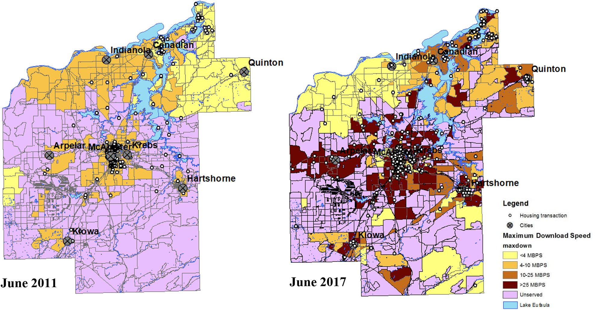
We created a series of maps capturing the maximum broadband speed available to each census block in both counties for each data update.⁹ This allowed us to examine spatial patterns in the deployment of broadband. A snapshot of the beginning and end of the six-year time span echoes the increased broadband coverage depicted in Tables 1 and 2 (Figures 2 and 3). This is especially prominent in the less populated Woods County (Figure 2), where the census blocks without providers of high-speed Internet generally disappear between 2011 and 2017. Not surprisingly, the increased speeds observed are centered on the highlighted, larger cities for both counties.

Figure 2.

Fixed broadband access—Woods county (June 2011 vs. June 2017).

Figure 3.

Fixed broadband access—Pittsburg county (June 2011 vs. June 2017).

Table 1 and 2 along with the visual counterparts (Figure 2 and 3) tell a consistent story of increasing download speeds over time for both counties. It is important to note the discrepancy that occurs as the data source transitioned from the NBM to FCC after June 2014 (dashed line in Tables 1 and 2). Notably, there is an implausible increase in unserved blocks for Pittsburg County (Table 2) and jump to full broadband coverage in Woods County (Table 1) in December 2014. Such discrepancies are not unexpected when a significant change in data collection methodology is experienced. The overall lower broadband coverage for Pittsburg County could also be explained by the higher presence of wetland and physical barriers that require more specialized engineering techniques for broadband deployment (Zager 2011). The white dots on the map indicate the housing transaction data for each corresponding period.¹⁰

Housing transaction data were collected through the county record system PvPlus, which has county assessor data on all property transactions within a county. Using these data platform, we specified the years (June 2011–December 2017) and counties of interest to obtain records of all property sales. The data collected included all residential sales and a series of descriptive characteristics for each house sold. Specific characteristics of interest include address, sale date, transaction price, number of bedrooms, bathrooms, acres, presence of fireplace, year built, garage square feet, and square feet of the home (Table 3). Similar to Molnar, Savage, and Sicker (2015), we deleted observations with no bathrooms, no bedrooms, and those with sale prices in the top 1 percent of the distribution. We further removed all observations with sales prices below $50,000 since such purchases are more likely to be salvage opportunities and may not represent a “move-in-ready” house. Additionally, we are only interested in single or multi-family homes, so all mobile homes were deleted.

Table 3.

Variable Descriptions.

Variable	Description	Data Source, Year(s)
Home characteristics
Price	Transaction price of house	PvPlus, 2011–2017
House_age	Age of house	PvPlus, 2011–2017
House_size	House size in square feet	PvPlus, 2011–2017
Garage_size	Garage size in house in square feet	PvPlus, 2011–2017
Fireplace	House has fireplace = 1, 0 otherwise	PvPlus, 2011–2017
Bathrooms	Number of bathrooms in house	PvPlus, 2011–2017
Bedrooms	Number of bedrooms in house	PvPlus, 2011–2017
Acres	Number of acres included in transaction	PvPlus, 2011–2017
Distance	The distance (in miles) the house is from the county seat (Pittsburg Co.= McAlester; Woods Co. = Alva)	Calculated using Geographic Information Software (GIS)
Year fixed effects	Dummy if house was sold in (Year) = 1, 0 otherwise. 2011 = base	PvPlus, 2011–2017
School district fixed effects	Dummy for school district associated with house (3 districts in Woods Co., 17 in Pittsburg Co.)	Oklahoma Center for Spatial Analysis; GIS
Quarter of sale fixed effects	Dummy for quarter of sale (Q1 = Jan–Mar; Q2 = Apr–June; Q3 = Jul–Sep; Q4 = Oct–Dec). Q4 = base	PvPlus, 2011–2017
Census block–group level characteristics
Population	Total population of each census block group	ACS, 5-year estimates, 2012–2016
Education	Mean years of schooling for the population 25 and older of each census block group	ACS, 5-year estimates, 2012–2016
HH_I	Median household income in the past 12 months of each census block group	ACS, 5-year estimates, 2012–2016
House_units	Number of houses in each census block group	ACS, 5-year estimates, 2012–2016
Pop growth	Population growth between 2000 and 2010 (pct. change), by census block group	Decennial Census, 2000 & 2010
Pct White	Percentage of population that is white, by census block group	ACS, 5-year estimates, 2012–2016
Age	Median age of population in each census block group	ACS, 5-year estimates, 2012–2016
Broadband levels
Maxdown	Maximum download speed available in each census block	NBM (June 2011 to June 2014); FCC (Dec. 2014 to June 2017)
BB_10	If maxdown is equal to 10–24 Mbps download speed = 1, otherwise 0	NBM (June 2011 to June 2014); FCC (Dec. 2014 to June 2017)
BB_25	If maxdown is equal to 25–49 Mbps download speed = 1, otherwise 0	NBM (June 2011 to June 2014); FCC (Dec. 2014 to June 2017)
BB_50	If maxdown is equal to 50–999 Mbps download speed = 1, otherwise 0	NBM (June 2011 to June 2014); FCC (Dec. 2014 to June 2017)
BB_1G	If maxdown is equal to 1G (1,000 Mbps) download speed = 1, otherwise 0	NBM (June 2011 to June 2014); FCC (Dec. 2014 to June 2017)

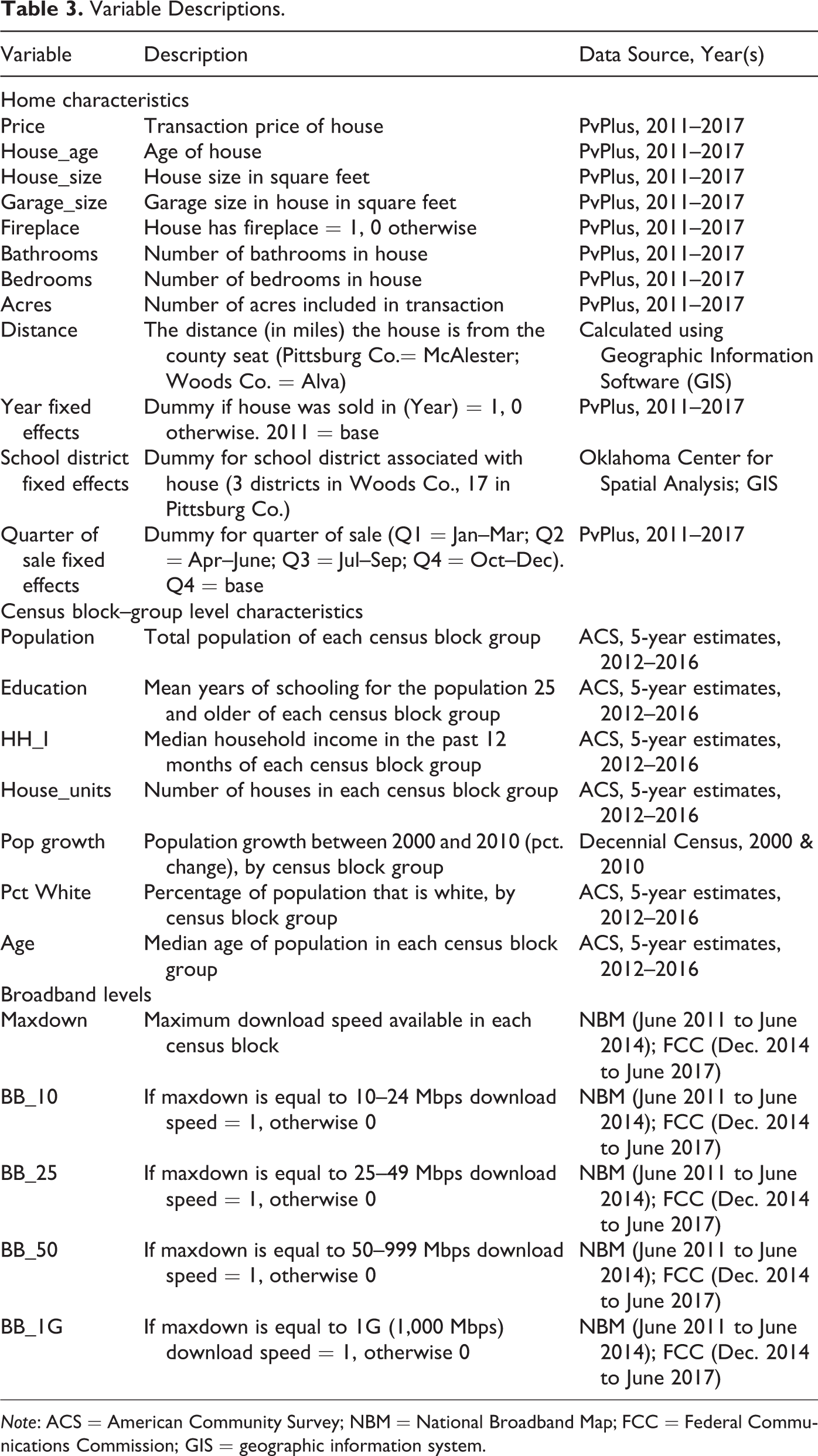
Note: ACS = American Community Survey; NBM = National Broadband Map; FCC = Federal Communications Commission; GIS = geographic information system.

In addition to the broadband variables of interest and the housing transaction characteristics, we gathered resident characteristics at the census block group level. On average, there are around 445 houses per census block group in Woods County and 545 houses per census block group in Pittsburg County. Data on population, education, household income, number of housing units, percentage of population that is white, and age were collected from the Census Bureau’s ACS (5-year, 2012–2016 estimates), at the lowest-level geography (block group) that is publicly available (Table 3). We also gathered data on the 2000–2010 population change at the block group level. Aggregate characteristics of the neighborhood, including socioeconomic variables such as race, income or education levels, and recent population growth could affect individual house transactions and therefore need to be controlled for in our model (DeBruyne and Hove 2013). The resident characteristics at the census block group level also help control for the spatial nature of housing data. Potentially omitted variables include crime rates and whether homes are located inside city limits, which we do not include due to data limitations.¹¹ However, we do control for the distance the home is from the county seat. Additionally, for Pittsburg County, we controlled for lake proximity, specifically Lake Eufaula, by creating a dummy variable for census block groups contiguous to the body of water. Finally, we include dummy variables for the school district each house is a part of (three districts exist in Woods; seventeen exist in Pittsburg) and also for the quarter the sale took place in.¹²

In order to be mapped, the given house transaction addresses were geocoded and converted to latitude and longitude coordinates. Each dot on a map represents a single housing transaction. Once mapped, the maximum download speed available to each home was obtained by overlaying the housing transaction with the appropriate data from the NBM or FCC. The housing transactions for each period are largely clustered around the labeled towns and cities for both counties (Figure 2 and 3); however, transactions do exist in the more rural portions of both counties. Geographic Information Software was used to calculate the distance in miles from each house to their respective county seat and to determine the school district associated with each house.

Summary statistics are reported for the housing transactions in each county over the six-year period (Table 4). The more populated Pittsburg County has a higher number of housing sales (n = 2,215) and higher average housing units at the census block group level than Woods County (n = 490). Both counties have similar mean transaction prices, house and garage size, number of bathrooms, and acres.¹³ On average, Woods County has significantly older homes, with higher levels of neighborhood education and income. The average broadband download speed (“maxdown”) is higher for Woods County, which is as expected given the maps in Figures 1 and 2.

Table 4.

Summary Statistics by County, 2011–2017.

Variable	Woods Co.					Pittsburg Co.
Variable	Obs.	Mean	Std. Dev.	Min	Max	Obs.	Mean	Std. Dev.	Min	Max
Price	490	$126,188	$72,839	$50,000	$450,000	2,215	$150,038	$95,861	$50,000	$600,000
House_age	490	61.98	25.39	1.00	115.00	2,215	36.41	24.95	0.00	137.00
House_size	490	1,660	629	60	5,651	2,215	1,721	612	188	6,352
Garage_size	490	331	271	0	1,240	2,215	387	322	0	3,600
Fireplace	490	0.41	0.49	0	1	2,215	0.36	0.48	0	1
Bathrooms	490	1.91	0.73	1	5	2,215	1.84	0.63	1	6
Bedrooms	490	2.92	0.84	1	9	2,215	3.03	0.82	1	15
Acres	490	3.57	20.33	0	235	2,215	6.22	24.81	0	408
Distance	490	3.49	6.40	0.06	30	2,215	8.62	8.96	0	30
Population	490	939	376	458	1,713	2,215	1,399	663	474	2,775
Education	490	13.61	0.99	12.24	15.05	2,215	12.98	0.57	11.47	14.07
HH_I	490	$61,698	$13,799	$41,386	$84,837	2,116^a	$48,734	$14,640	$19,327	$84,479
House_units	490	448	111	315	651	2,215	889	828	267	2,900
Pop growth (00-10)	490	−0.02	0.08	−0.16	0.212	2,215	0.15	0.33	−0.51	0.98
Pct White	490	0.88	0.08	0.76	0.98	2,215	0.76	0.09	0.42	0.90
Age	490	37.73	8.55	26.40	52.70	2,215	43.64	8.73	26.90	59.00
Maxdown	490	132.50	283.91	0	1,000	2,215	49.72	63.43	0	1,000

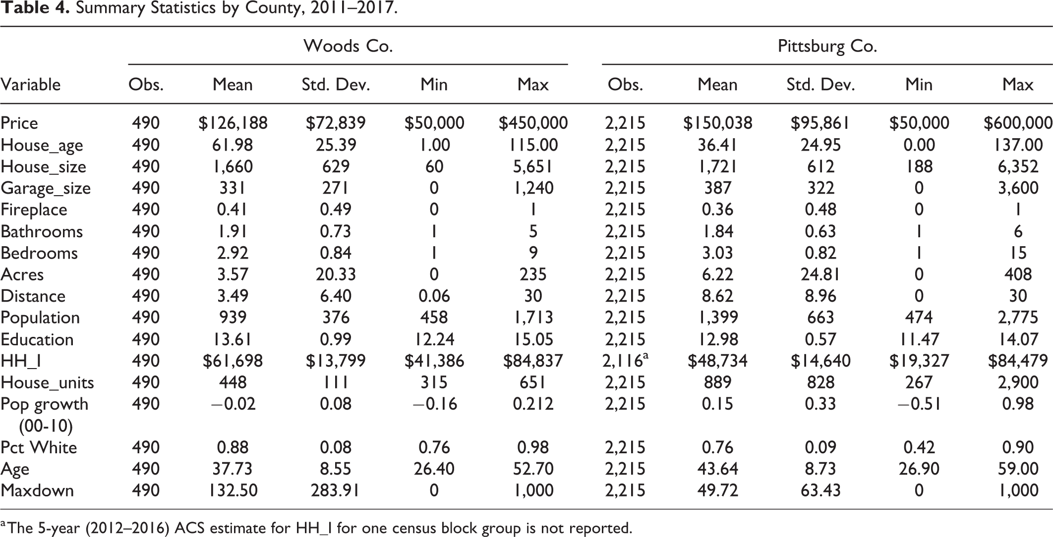
^a The 5-year (2012–2016) ACS estimate for HH_I for one census block group is not reported.

Yearly averages for housing prices and maximum broadband speeds available generally show increases in speeds over time (dramatically so in the more recent years), and housing prices that mostly increase monotonically for Woods but show considerable variation for Pittsburg (Table 5). These summary statistics and comparisons across years give us some insights into the potential relationship between housing prices and broadband availability, but we need to incorporate more formal empirical methods to isolate the impact of broadband on the purchase price.

Table 5.

Price and Maximum Download by Year and County.

	Woods					Pittsburg
Year	Obs.	Mean	Std. Dev.	Min^a	Max	Obs.	Mean	Std. Dev.	Min^a	Max
Price
2011	31	$109,717	$50,646	$52,000	$220,000	121	$139,802	$76,685	$50,000	$410,000
2012	68	$115,003	$72,301	$50,000	$393,000	241	$130,640	$73,846	$50,000	$450,000
2013	84	$118,326	$81,373	$50,000	$395,000	268	$142,250	$86,575	$50,000	$545,000
2014	69	$120,486	$66,041	$50,000	$400,000	327	$143,155	$88,096	$50,000	$575,000
2015	82	$134,933	$78,250	$50,000	$400,000	372	$165,214	$106,883	$50,000	$600,000
2016	79	$137,291	$70,558	$50,000	$390,000	419	$154,846	$101,903	$50,000	$600,000
2017	77	$135,678	$71,583	$50,000	$450,000	467	$155,587	$103,333	$50,000	$571,000
Maxdown (Mbps)
2011	31	8.71	2.65	0	10	121	7.55	3.75	0	10
2012	68	8.65	3.00	0	10	241	6.38	3.94	0	10
2013	84	10.37	9.54	0	50	268	5.82	3.43	0	10
2014	69	13.48	13.17	0	50	327	13.73	57.05	0	1,000
2015	82	105.62	229.79	3	1,000	372	64.32	46.97	0	105
2016	79	273.13	343.35	3	1,000	419	71.54	46.69	0	105
2017	77	416.06	434.71	2	1,000	467	109.21	76.93	0	200

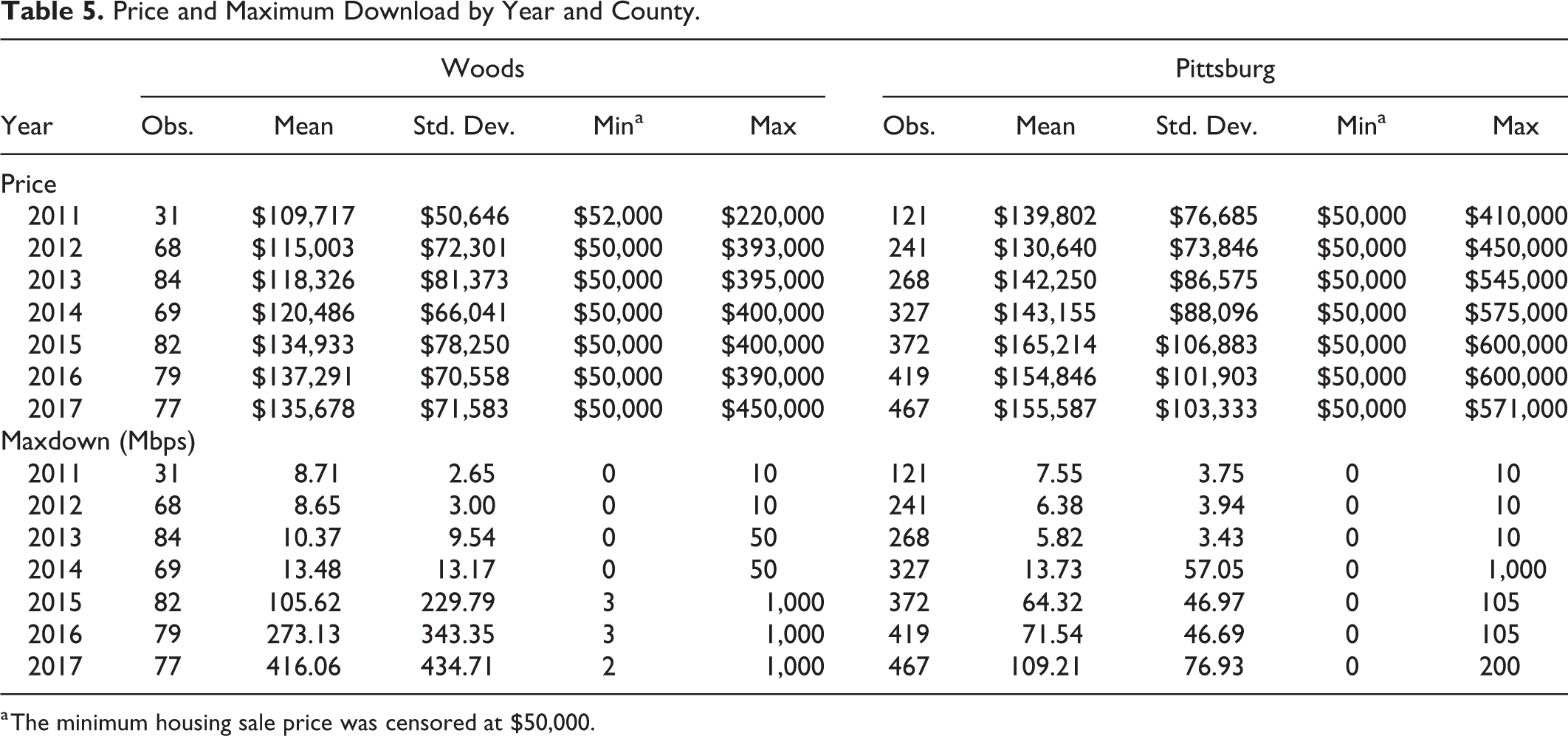
^a The minimum housing sale price was censored at $50,000.

Hedonic Model

Consumer theory states that consumers obtain utility not from simply consuming goods themselves, but rather from the various individual characteristics that compose the goods (Rosen 1974). Hedonic price models are well established in the economics literature, especially for evaluating home values (Sirmans, Macpherson, and Zietz 2005; Stetler, Venn, and Calkin 2010). A hedonic price function is a regression of the observed price of a commodity or service against its attributes (Lucas 1975). The parameters of the model can be estimated using data collected on the characteristics of a good in a given market. For this article, the amenities the home possesses serve as the characteristics of the home, and the home itself is our composite good of interest. Specifically, we are interested in how the characteristic of high-speed broadband availability impacts the housing transaction.

The hedonic pricing model can be estimated using OLS. Parameters are estimated by regressing the price of a home on the characteristics of the home. Following the methodology laid out in Molnar, Savage, and Sicker (2015), we use the following hedonic housing price equation,

\log P_{i k t j} = X_{i} β + Z_{k} ϕ + δ_{t} + B B_{j} α + ∊_{i k t j},

where P is the transaction price for home $i =$ 1, 2,…, n in census block j = 1, 2,… $J$ , in census block group k = 1, 2,…K at time t; X is a vector of home individual characteristics; Z is a vector of resident and housing characteristics at the census block group level; $δ$ is a time fixed effect for year t (2012–2017); $B B$ is the broadband variable of interest; $∊$ is a normally distributed error term; and $β$ , f, $δ$ , and $α$ are parameters to be estimated. ¹⁴ This OLS regression is run separately for each county. The specific parameter of interest is $α$ , where a positive and significant parameter value indicates that higher available download speeds have a positive effect on the price of the home, holding everything else constant.

Spatial Econometric Approach

As our literature review notes, traditional OLS approaches may not capture important spatial patterns that are common in housing markets, with house prices often mirroring their neighbor’s values. We can test for the presence of spatial patterns in the residuals of our regression; Lagrange multipliers can be used to assess whether a spatial lag or spatial error model is more appropriate (Anselin 1990). Many hedonic papers use the spatial lag equation:

\log P_{i k t j} = ρ W l o g P_{m k t j} + X_{i} β + Z_{k} ϕ + δ_{t} + B B_{j} α + ∊_{i k t j},

where $ρ$ is the spatial dependence parameter and W is a spatial weight matrix representing which of the observations m is considered a neighbor to observation i. In practice a variety of spatial weight matrices can be used, but a typical approach with housing data is to use distance-based matrices where only neighbors below a threshold are assigned nonzero weight. The inclusion of the $ρ$ term captures any potential impact of neighboring housing values, and may also influence the remaining coefficient values and signs.

Results

The OLS estimates of the hedonic housing price model for Woods County are presented in Table 6, and the results for Pittsburg County are in Table 7. Starting with a baseline model of home characteristics (i), we then run a series of six other model specifications for each county. We add in additional controls for each model to test the robustness of the broadband parameters of interest. The continuous broadband variable (Maxdown) is included in models (ii), (iv), and (vi). We convert the continuous broadband variable to categorical variables denoting the highest speed level available each house, and these are included in models (iii), (v), and (vii). Models (iv) and (v) introduce yearly dummy variables. Our preferred models are (vi) and (vii), which further include census block group resident and housing characteristics and incorporate the spatial lag specification in equation (2). The distance in miles each housing transaction is from the county seat is also included in models (ii)–(vii). For Pittsburg County the lake dummy variable is included for all model specifications. We note that the R ² values increase for each subsequent model specification across both counties, although the pseudo-R ² values for the spatial specifications in (vi) and (vii) are not directly comparable to the OLS versions. The specific results for each county and interpretation of the coefficients are discussed below.¹⁵

Table 6.

Ordinary Least Squares and Spatial Lag Estimates of Home Prices for Woods County, Oklahoma.

Variable	Dependent Variable: lnPrice
Variable	(i)	(ii)	(iii)	(iv)	(v)	(vi)	(vii)
House_age^a	−0.068*** 0.025	−0.076*** 0.025	−0.080*** 0.026	−0.075*** 0.025	−0.069*** 0.026	−0.081*** 0.025	−0.076*** 0.025
House_age²	0.002*** 0.002	0.003*** 0.002	0.003*** 0.002	0.003*** 0.002	0.002*** 0.002	0.004* 0.002	0.004* 0.002
House_size	0.283*** 0.099	0.329*** 0.100	0.323*** 0.100	0.331*** 0.100	0.310*** 0.100	0.299*** 0.097	0.277*** 0.098
House_size²	−0.008 0.021	−0.015 0.021	−0.014 0.021	−0.016 0.021	−0.012 0.021	−0.009 0.020	−0.005 0.020
Garage_size^b	0.191*** 0.067	0.185*** 0.066	0.185*** 0.067	0.185*** 0.067	0.197*** 0.067	0.196*** 0.068	0.199*** 0.068
Fireplace	0.148*** 0.039	0.138*** 0.038	0.140*** 0.039	0.143*** 0.038	0.147*** 0.038	0.130*** 0.038	0.132*** 0.038
Bathrooms	0.127*** 0.031	0.118*** 0.031	0.114*** 0.032	0.114*** 0.032	0.112*** 0.032	0.081*** 0.030	0.081*** 0.030
Acres	0.004*** 0.001	0.005*** 0.001	0.004*** 0.001	0.004*** 0.001	0.004*** 0.001	0.004*** 0.001	0.004*** 0.001
Distance		−0.006**0.003	−0.007**0.003	−0.007**0.003	−0.0050.003	−0.0040.013	−0.0040.013
Maxdown		0.0000.000		0.0000.000		0.0000.000
BB_10			−0.0300.061		0.0520.066		0.0770.072
BB_25			−0.0980.143		−0.1770.144		−0.1890.141
BB_50			0.0270.057		−0.0950.067		−0.0490.075
BB_1G			0.0460.076		−0.0930.086		−0.0240.094
Year Fixed Effects				Yes	Yes	Yes	Yes
lnPopulation						−0.1110.171	−0.1240.171
Education						0.0530.051	−0.0510.052
lnHH_I						0.4460.442	0.4780.441
lnHouse_units						0.0970.219	0.1370.227
Pop growth (00-10)						−0.6500.472	−0.6300.478
Pct White						−0.5640.587	−0.5580.591
Age						−0.0070.010	−0.0070.009
School district fixed effects						Yes	Yes
Quarter of sale fixed effects						Yes	Yes
ρ (spatially lagged dep. variable)						0.435***0.144	0.409***0.146
Intercept	11.117***0.133	11.127***0.133	11.166***0.142	11.058***0.147	11.006***0.159	2.8293.344	2.5263.342
R ²	.500	.508	.510	.520	.525	.594	.595

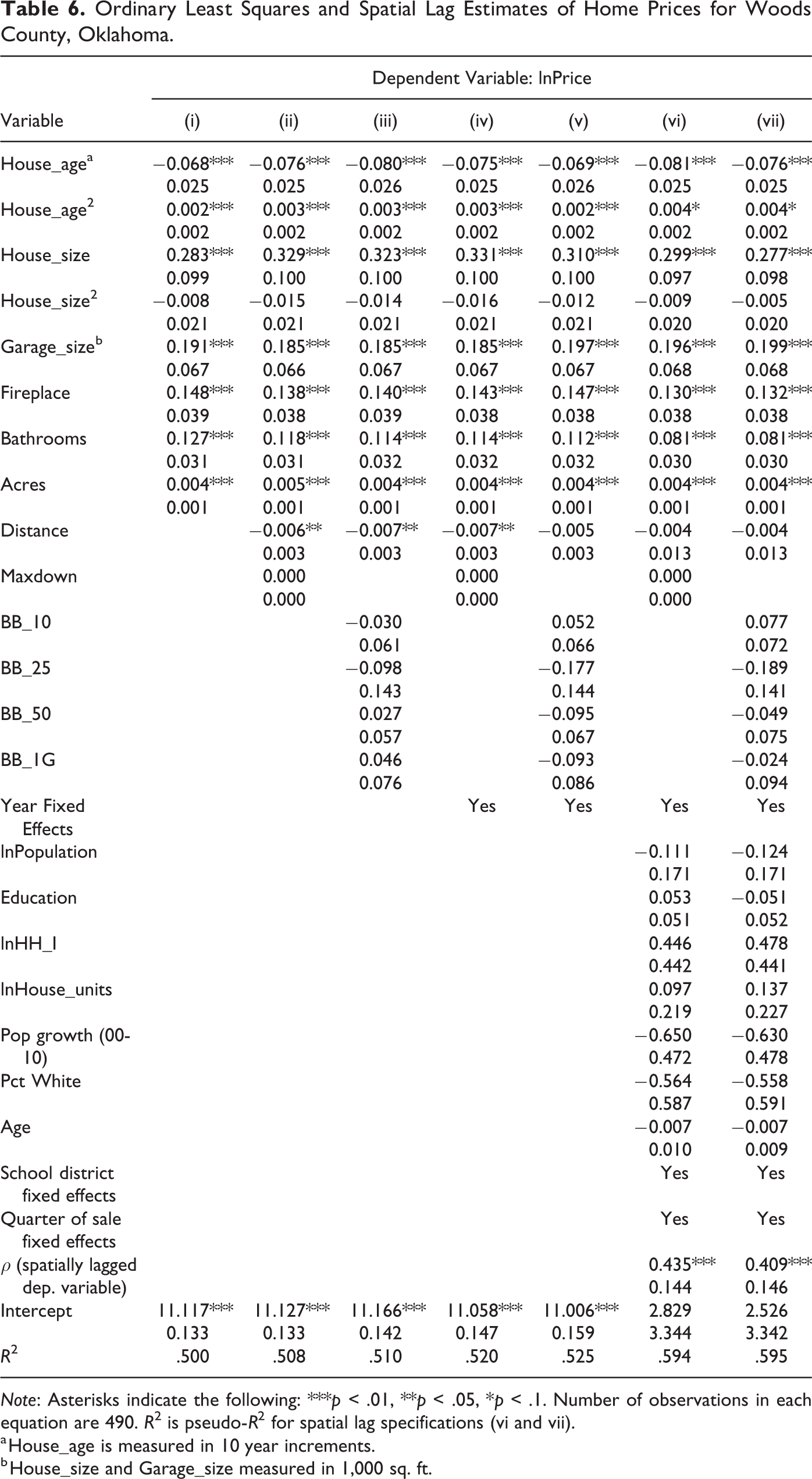
Note: Asterisks indicate the following: ***p < .01, **p < .05, *p < .1. Number of observations in each equation are 490. R ² is pseudo-R ² for spatial lag specifications (vi and vii).

^a House_age is measured in 10 year increments.

^b House_size and Garage_size measured in 1,000 sq. ft.

Table 7.

Ordinary Least Squares and Spatial Lag Estimates of Home Prices for Pittsburg County, Oklahoma.

Variable	Dependent Variable: lnPrice
Variable	(i)	(ii)	(iii)	(iv)	(v)	(vi)	(vii)
House_age^a	−0.103***0.012	−0.099***0.012	−0.100***0.012	−0.098***0.012	−0.098***0.012	−0.060***0.012	−0.061***0.012
House_age²	0.005***0.001	0.005***0.001	0.005***0.001	0.005***0.001	0.005***0.001	0.003***0.001	0.003***0.001
House_size^b	0.459***0.059	0.459***0.059	0.457***0.059	0.461***0.059	0.458***0.059	0.418***0.057	0.418***0.057
House_size²	−0.054***0.012	−0.054***0.012	−0.054***0.012	−0.054***0.012	−0.054***0.012	−0.054***0.012	−0.054***0.012
Garage_size^b	0.204***0.031	0.210***0.031	0.209***0.031	0.211***0.031	0.209***0.031	0.175***0.029	0.175***0.029
Fireplace	0.157***0.022	0.157***0.022	0.156***0.022	0.155***0.022	0.154***0.022	0.101***0.021	0.100***0.021
Bathrooms	0.083***0.022	0.082***0.022	0.083***0.022	0.082***0.022	0.084***0.022	0.059***0.021	0.059***0.021
Acres	0.004***0.000	0.004***0.000	0.004***0.000	0.004***0.000	0.004***0.000	0.004***0.000	0.004***0.000
Lake	0.122***0.020	0.092***0.025	0.090***0.025	0.090***0.025	0.086***0.025	−0.0000.044	−0.0030.044
Distance		0.004***0.001	0.004***0.001	0.0030.014	0.003**0.001	−0.0030.004	−0.003−0.004
Maxdown		0.000***0.000		0.0000.000		0.0000.000
BB_10			−0.0330.026		−0.0330.027		−0.0120.026
BB_25			−0.0390.091		−0.0550.092		−0.1640.157
BB_50			0.047**0.022		−0.0080.029		−0.0060.029
BB_1G			0.3320.441		0.3420.441		0.1050.412
Year fixed effects				Yes	Yes	Yes	Yes
lnPopulation						0.0320.091	0.0260.091
Education						−0.0110.029	−0.0110.029
lnHH_I						0.1090.069	0.1060.069
lnHouse_units						0.0580.083	0.0670.084
Pop growth (00-10)						−0.067*0.037	−0.065*0.037
Pct_White						0.258*0.147	0.259*0.147
Age						−0.0010.002	−0.0010.002
School district fixed effects						Yes	Yes
Quarter of sale fixed effects						Yes	Yes
ρ (spatially lagged dep. variable)						0.356***0.027	0.359***0.027
Intercept	11.058***0.071	11.000***0.073	11.016***0.073	10.988***0.082	11.016***0.084	4.704***0.664	5.164***0.579
R ²	.388	.392	.392	.395	.395	.486	.486

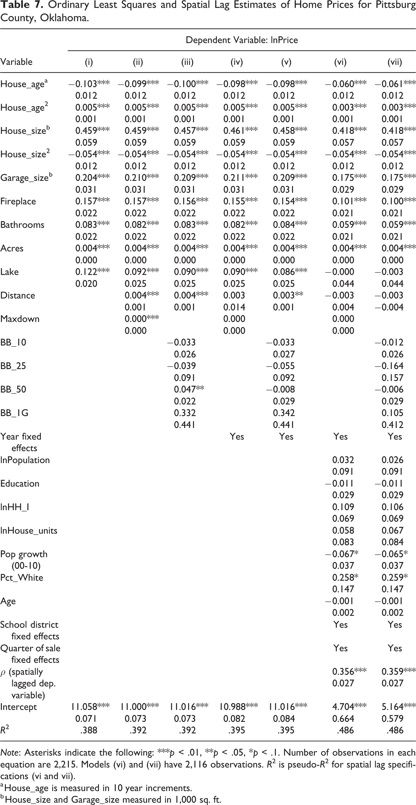
Note: Asterisks indicate the following: ***p < .01, **p < .05, *p < .1. Number of observations in each equation are 2,215. Models (vi) and (vii) have 2,116 observations. R ² is pseudo-R ² for spatial lag specifications (vi and vii).

^a House_age is measured in 10 year increments.

^b House_size and Garage_size measured in 1,000 sq. ft.

Woods County

The initial signs on the housing characteristics in model (i) are as expected. House age², house size, garage size, presence of a fireplace, number of bathrooms, and total acres are positive and significant across all model specifications.¹⁶ This suggests that as the square footage and number of bathrooms increase, the sale price of the home increases. Specifically, an additional bathroom is associated with a 12.7 percent higher home value. Evaluated at the mean home price for Woods County ($126,188; Table 4), this translates to approximately a $16,025 increase per bathroom.¹⁷ House age is negative and significant across all models, suggesting that value of a house decreases with age. Distance from the county seat was added beginning in model (ii) and is found to be negative and significant across the preliminary model specifications, indicating a lower price for houses that are further away from the county seat. Each of these results is consistent with our a priori expectations and other hedonic literature (Cohen and Coughlin 2008; Molnar, Savage, and Sicker 2015; Ready and Abdalla 2005; Palmquist, Roka, and Vukina 1997).

We control for the price differences over time by adding a yearly dummy variable indicating the year the house was sold (models (iv)–(vii)). Our preferred models are (vi) and (vii), which add in controls for neighborhood characteristics, quarter of sale date, and school district fixed effects in addition to the inclusion of a spatially lagged dependent variable.¹⁸ The yearly coefficients for 2016 and 2017 are positive and statistically significant for all model specifications (not shown); however, none of the controls at the census block group level were significant. The additional fixed effect variables (quarter of sale and school district) also proved insignificant in Woods County. Importantly, the spatial parameter was highly statistically significant, suggesting that nearby housing values do impact the final transaction price. Notably, however, the main household characteristic parameters in OLS models (i)–(v) do not dramatically differ from those in the spatial specifications (vi) and (vii).

The broadband variables of interest are included in two distinct ways—maxdown (a continuous measure of the maximum speed available for that house) and BB_10, BB_25, BB_50, and BB_1G (mutually exclusive dummy variables denoting the category of maximum speed available). The coefficient on Maxdown across models (ii), (iv), and (vi) is very small and not significant. Similarly, the speed threshold dummy variables are not significant in models (iii), (v), or (vii). As such, the results in Table 6 offer no support for the hypothesis that broadband availability impacts housing values in Woods County.

Pittsburg County

Examining the first model specification controlling only for housing characteristics, we again find that house age², house size, garage size, presence of a fireplace, number of bathrooms, acres, and being located near the lake all positively (and significantly) influence the home price. For example, a Pittsburg County home with a fireplace is associated with a 15.7 percent higher home value in model (i). Evaluated at the mean housing price of $150,038 (Table 4), this equates to around a $23,500 increase in transaction price. This fireplace coefficient is similar to some hedonic studies (Cohen and Coughlin 2008), but higher than others (Palmquist, Roka, and Vukina 1997), and may serve as a proxy for overall housing quality. House age and house size² are negative and significant across all models. Interestingly, for model specifications (ii), (iii), and (v) distance to the county seat is found to be positive and significant, suggesting homes farther away from the county seat are associated with a higher house sale price. This counterintuitive result could be attributed to the presence of the state penitentiary located in the county seat of McAlester. However, after controlling for year, block group, and spatial effects, the distance parameter becomes negative and insignificant, similar to the Woods County results. Unlike Woods County, no year effects are significant (not shown); however, lower population growth and percentage of population that is white at the census block group level are associated with increases in housing transaction price. Sales in Quarter 1 lowered the sale price relative to Quarter 4, and several school districts were associated with higher prices relative to the smallest district (not shown). Again, the spatial parameters in models (vi) and (vii) are highly statistically significant, and these models notably remove the significance associated with the distance and lake variables.¹⁹

The broadband variables for Pittsburg County show varying but very limited results, with positive and significant impacts only appearing in preliminary models. Notably, the continuous broadband variable, while very small, is positive and significant at the p < .01 level for model (ii), suggesting that homes with faster speeds in Pittsburg County receive a slight sale premium. After controlling for year and county block group effects (models (iv) and (vi)), the parameter stays small and positive, but is no longer significant. Turning to the categorical broadband variable, there is a positive and significant relationship between house sale prices and homes equipped with broadband at speeds between 50-99 Mbps (model (iii)), before controlling for year effects or block-group characteristics. However, this positive and significant broadband premium disappears when controlling for year and county block group effects, and our preferred specification (model vii) shows no impact of broadband on housing prices. This is similar to the lack of significance displayed in the Woods County models. Again, we note that our spatial models appear to be the most appropriate specifications, with Moran’s I tests of the residuals finding no evidence of spatial autocorrelation (p = 0.41 and p = 0.42 for models (vi) and (vii)).

Conclusions

This article has sought to determine if the availability of high-speed Internet has a positive impact on housing prices in rural areas. Broadband deployment and housing transactions for two rural Oklahoma counties from 2011 to 2017 are used, with OLS and spatial hedonic pricing models finding strong impacts for traditional housing characteristics, but not for broadband. In both of our counties, no such premium is uncovered for any type of broadband availability, regardless of whether it is measured in terms of maximum speed or by speed category. These results underscore that a robust and sizable broadband premium for rural households is far from a certainty and may be nonexistent in cases where diffusion has been significant.

Overall, the results from both Oklahoma counties suggest that no measurable premium exists for broadband access across these counties, but that one may exist in other rural areas depending on individual county settings. Woods County never saw a broadband premium across any of our six model specifications, while in the more populated Pittsburg County, a threshold of 50–99 Mbps was positively significant in our base model. Both counties saw major improvements in broadband availability over the last decade; it could be the case that areas with lower levels of infrastructure are a more appropriate place to see impacts to housing uncovered in approaches such as ours (i.e., the very limited places with broadband access are rewarded with housing price premiums). We do note that much of the recent (i.e., after 2015) investment in broadband networks have come at faster (> 50 or even > 100 Mbps) speeds, and that such networks may not have had time to demonstrate an impact in our data. At least one recent analysis (Lobo et al. 2020) has demonstrated that these very high-speed networks can have a measureable impact on employment in rural areas.

The differing hedonic results across Woods and Pittsburg counties suggest that factors impacting housing prices vary across county and context. While broadband availability was generally shown to be insignificant, other housing characteristics were shown to impact housing prices differently. In particular, Woods County residents seem to highly value additional bathrooms, while the premium on housing size is much larger in Pittsburg County. Other factors also differ, with yearly effects being highly significant in Woods County (but not in Pittsburg), and block group–level variables being significant in Pittsburg (but not Woods). We previously noted the presence of a lake and a prison in Pittsburg County, but these characteristics were not important contributors to housing price in our final model—likely due to the inclusion of a spatial lag term.

These results are interesting and suggest significant complexity and variation among housing prices in rural counties. Federal government assistance programs continue to focus on providing broadband infrastructure investments (Office of Management and Budget, Budget of the U.S. Government 2018). The Rural Utilities Service at the US Department of Agriculture (USDA) houses three ongoing assistance programs specifically dedicated to financing broadband deployment (Kruger 2019). Additionally, the FCC provides broadband assistance for unserved and underserved communities via the Connect America Fund (CAF), now in Phase II and distributing $1.98 billion over ten years (FCC 2019). For Oklahoma specifically, $336.1 million was allocated through the USDA over eight years (2009–2016), and another $2.5 million was awarded in Phase I of the FCC’s CAF from 2012 to 2014 (Kruger 2019; FCC 2015). Policy makers and researchers need to be cautious of treating houses, consumers, and rural areas as homogeneous groups that will all benefit equally from these types of investments. Our results show that some of the outcomes assumed to result from such investment (higher housing values, e.g.) may not accrue in all instances.

A limitation of our study—and avenue for future research—is the lack of inclusion of satellite or mobile broadband connections. Data from the 2013–2017, ACS suggests that satellite connectivity is about the same in each county, comprising roughly 14 percent of all connected households in each case (higher than the 10 percent state average). Some residents may simply be assuming they can get satellite coverage if a potential residence does not have good terrestrial access.²⁰ While this study did not examine mobile Long Term Evolution connections, it is important to note that cellular networks are usually limited to speeds of up to 10 Mbps, come with monthly data caps, and are generally not as useful as wired counterparts (Anderson and Horrigan 2016).²¹ However, mobile coverage was significantly better in Pittsburg County and could be playing a role in the lack of impact seen for traditional wireline access.²² Endogeneity is another limitation of our study, since Internet providers might take local housing prices into account when deciding their service area. Prieger (2003) used an instrumental variable (IV) of terrain slope, but in our case, this might also affect housing prices. Molnar, Savage, and Sicker (2015) also note the difficulty of finding an appropriate IV in broadband work. Another limitation of this work is the fact that only two rural Oklahoma counties were examined. Further research could explore alternative categories of rural counties and assess why the results in other locations are either similar to or different from those found here.

Adding to the growing broadband literature, this article is the first to examine the relationship between broadband availability and housing prices for rural counties specifically at the individual household level. Our primary results indicate that high-speed broadband does not have a measurable impact on house sale prices in at least some instances in rural America. Broadband availability is important for rural households for a variety of reasons; however, each household has a different value they are willing to place on accessing high-speed Internet. Our analysis of housing prices in two rural Oklahoma counties finds no support for the existence of a broadband premium.

Supplemental Material

Appendix_A - Home Is Where the Internet Is? High-speed Internet’s Impact on Rural Housing Values

Appendix_A for Home Is Where the Internet Is? High-speed Internet’s Impact on Rural Housing Values by Kelsey L. Conley and Brian E. Whitacre in International Regional Science Review

Footnotes

Declaration of Conflicting Interests

The author(s) declared no potential conflicts of interest with respect to the research, authorship, and/or publication of this article.

Funding

The author(s) received no financial support for the research, authorship, and/or publication of this article.

ORCID iDs

Kelsey L. Conley

Brian E. Whitacre

Supplemental Material

Supplemental material for this article is available online.

Notes

References

Ahlfeldt

Koutroumpis

Valletti

. 2014. “Speed 2.0: Evaluating Access to Universal Digital Highways.” CEIS Working Paper No. 328. Accessed March 12, 2019. http://www.spatialeconomics.ac.uk/textonly/serc/publications/download/sercdp0161.pdf.

Anderson

2018. “About a Quarter of Rural Americans say Access to High-speed Internet is a Major Problrm.” Post for PEW Research Center. Accessed November 9, 2018. http://www.pewresearch.org/fact-tank/2018/09/10/about-a-quarter-of-rural-americans-say-access-to-high-speed-internet-is-a-major-problem/.

Anderson

Horrigan

. 2016. “Smartphones Help Those Without Broadband Get Online, But Don’t Necessarily Bridge the Digital Divide.” Post for PEW Internet Research Center. Accessed November 9, 2018. http://www.pewresearch.org/fact-tank/2016/10/03/smartphones-help-those-without-broadband-get-online-but-dont-necessarily-bridge-the-digital-divide/.

Anselin

1990. “Some Robust Approaches to Testing and Estimation in Spatial Econometrics.” Regional Science and Urban Economics 20:141–63.

Atasoy

2013. “The Effects of Broadband Internet Expansion on Labor Market Outcomes.” Journal of Economic Perspectives 24:207–32.

Balthrop

A. T.

Hawley

. 2017. “I Can Hear My Neighbors’ Fracking: The Effect of Natural Gas Production on Housing Values in Tarrant County, TX.” Energy Economics 61:351–62.

Basu

Thibodeau

T. G.

. 1998. “Analysis of Spatial Autocorrelation in House Prices.” Journal of Real Estate Finance and Economics 17:61–85.

Baum-Snow

Nathaniel

Kahn

Matthew E.

. 2000. “The Effects of New Public Projects to Expand Urban Rail Transit.” Journal of Public Economics 77:241–63.

Bennett

Loomis

. 2015. “Are Housing Prices Pulled Down or Pushed Up by Fracked Oil and Gas Wells? A Hedonic Price Analysis of Housing Values in Weld County, Colorado.” Society & Natural Resources 28:1168–86.

10.

Boxall

P. C.

Chan

W. H.

McMillan

M. L.

. 2005. “The Impact of Oil and Natural Gas Facilities on Rural Residential Property Values: A Spatial Hedonic Analysis.” Resource and Energy Economics 27:248–69.

11.

Brodkin

. 2015a. “Man Builds House, Then Finds Out Cable Internet Will Cost $117,000.” Ars Technica. Accessed September 5, 2018. https://arstechnica.com/information-technology/2015/09/man-builds-house-then-finds-out-cable-internet-will-cost-117000/.

12.

Brodkin

. 2015b. “Want Fiber Internet? That’ll be $383,500, ISP Tells Farm Owner.” Ars Technica. Accessed September 5, 2018. https://arstechnica.com/information-technology/2015/08/want-fiber-internet-thatll-be-383500-isp-tells-farm-owner/.

13.

Busby

Tanberk

. 2020. “FCC Reports Broadband Unavailable to 21.3 Million Americans, BroadbandNow Study Indicates 42 Million Do Not Have Access.” Broadband Now Research. Accessed February 3, 2020. https://broadbandnow.com/research/fcc-underestimates-unserved-by-50-percent.

14.

Cohen

J. P.

Coughlin

C. C.

. 2008. “Spatial Hedonic Models of Airport Noise, Proximity, and Housing Prices.” Journal of Regional Science 48:859–78.

15.

Conley

K. L.

Whitacre

. 2016. “Does Broadband Matter for Rural Entrepreneurs or ‘Creative Class’ Employees?” Review of Regional Studies 46:171–90.

16.

Crawford

2019. Fiber: The Coming Tech Revolution—And Why America Might Miss It. New Haven, CT: Yale University Press.

17.

Cromartie

. 2018. Rural America at a Glance, 2018 Edition. Washington, DC: US Department of Agriculture Economic Research Service. Accessed November 21, 2018. https://www.ers.usda.gov/publications/pub-details/?pubid=90555.

18.

Czernich

Falck

Kretschmer

Woessmann

. 2011. “Broadband Infrastructure and Economic Growth.” The Economic Journal 121:505–32.

19.

DeBruyne

Hove

J. V.

. 2013. “Explaining the Spatial Variation in Housing Prices: An Economic Geography Approach.” Applied Economics 42:1673–89.

20.

Deller

Whitacre

. 2019. “Broadband’s Relationship to Rural Housing Values.” Papers in Regional Science 98:2135–56.

21.

Devaraj

Sharma

Wornell

E. J.

Hicks

M. J.

. 2017. Human Development & Technology in US Counties: Technology Quality & Accessibility Considerations for Policy Makers. Muncie, IN: Ball State University. Accessed March 15, 2018. https://projects.cberdata.org/reports/HDTI-US-20171005.pdf.

22.

Dubin

R. A.

1988. “Estimation of Regression Coefficients in the Presence of Spatially Auto-correlated Error Terms.” Review of Economics and Statistics 70:466–74.

23.

Dutz

Orszag

Willig

. 2009. The Substantial Consumer Benefits of Broadband Connectivity for US Households. New York: Internet Innovation Alliance.

24.

FCC (Federal Communicaitons Commission). 2012. Eighth Broadband Progress Report. Washington, DC: Federal Communications Commission. Accessed April 8, 2019. https://www.fcc.gov/reports-research/reports/broadband-progress-reports/eighth-broadband-progress-report.

25.

FCC (Federal Communicaitons Commission). 2014. Types of Broadband Connections. Washington, DC: Federal Communications Commission. June 2014. Accessed September 13, 2018. https://www.fcc.gov/general/types-broadband-connections.

26.

FCC (Federal Communicaitons Commission). 2015. Connect America Fund Progress Portal. Washington, DC: Federal Communications Commission. November 2015. Accessed January 16, 2019. https://www.fcc.gov/general/connect-america-fund-progress-portal.

27.

FCC (Federal Communicaitons Commission). 2016. 2016 Broadband Progress Report. Washington, DC: Federal Communications Commission. Accessed June 21, 2018. https://www.fcc.gov/reports-research/reports/broadband-progress-reports/2016-broadband-progress-report.

28.

FCC (Federal Communicaitons Commission). 2018a. 2018 Broadband Deployment Report. Washington, DC: Federal Communications Commission. Accessed June 21, 2018. https://www.fcc.gov/reports-research/reports/broadband-progress-reports/2018-broadband-deployment-report.

29.

FCC (Federal Communicaitons Commission). 2018b. Eighth Measuring Broadband America Fixed Broadband Report. A Report on Consumer Fixed Broadband Performance in the United States. Washington, DC: Federal Communicaiton Commission, Office of Engineering and Technology. Dec. 14, 2018. Accessed January 16, 2019. https://www.fcc.gov/reports-research/reports/measuring-broadband-america/measuring-fixed-broadband-eighth-report.

30.

FCC (Federal Communicaitons Commission). 2019. 2019 Broadband Deployment Report. Washington, DC: Federal Communications Commission. Accessed June 21, 2019. https://docs.fcc.gov/public/attachments/FCC-19-44A1.pdf.

31.

FCC (Federal Communicaitons Commission). 2019. Connect America Fund Phase II Auction (Auction 903). Washington, DC: Federal Communications Commission. October 2019. Accessed October 3, 2019. https://www.fcc.gov/auction/903.

32.

Ford

2011. “Challenges in Using the National Broadband Map’s Data.” Phoenix Center Policy Bulletin 27:1–27.

33.

Geoghegan

Lynch

Bucholtz

. 2003. “Capitalization of Open Spaces into Housing Values and the Residential Property Tax Revenue Impacts of Agricultural Easement Programs.” Agricultural and Resource Economics Review 32:33–45.

34.

Gillet

Lehr

Osorio

Sirbu

. 2006. “Measuring the Economic Impact of Broadband Deployment.” Washington, DC: Final Report for Economic Development Administration.

35.

Goolsbee

Klenow

P. J.

. 2006. “Valuing Consumer Products by the Time Spent Using Them: An Application to the Internet.” American Economic Review 96:108–13.

36.

Government Accountability Office. 2009. “Current Boradband Measures Have Limitations and New Measures Are Promising but Need Improvement.” GAO Report GAO-10-49. Accessed June 21, 2018. http://www.gao.gov/assets/300/296726.pdf.

37.

Grubesic

T. H.

2012. “The U.S. National Broadband Map: Data Limitations and Implications.” Telecommunications Policy 36:113–26.

38.

Holt

Jamison

. 2009. “Broadband and Contributions to Economic Growth: Lessons from the US Experience.” Telecommunications Policy 33:575–81.

39.

Jayakar

Park

. 2013. “Broadband Availability and Employment: An Analysis of County-level Data from the National Broadband Map.” Journal of Information Policy 3:181–200.

40.

Kashian

Zenteno

. 2014. “The Impact of Broadband Deployment on Recreational and Seasonal Property Values – A Hedonic Model.” Working Paper, University of Wisconsin Whitewater Fiscal and Economic Research Center.

41.

Kim

Orazem

P. F.

. 2017. “Broadband Internet and New Firm Location Decisions in Rural Areas.” American Journal of Agricultural Economics 99:285–302.

42.

Knutson

2015. “How Fast Internet Affects Home Prices.” Wall Street Journal.

43.

Kolko

2010. “A New Measure of US Residential Broadband Availability.” Telecommunications Policy 34:132–43.

44.

Kruger

L. G

. 2019. “Broadband Loan and Grant Programs in the USDA’s Rural Utilities Service.” Congressional Research Service, RL33816, version 130. Accessed April 5, 2019. https://fas.org/sgp/crs/misc/RL33816.pdf.

45.

Liu

Hite

. 2013. “Measuring the Effect of Green Space on Property Value: An Application of the Hedonic Spatial Quantile Regression.” Conference paper for the Southern Agricultural Economics Association, Orlando, FL. Accessed August 16, 2018. https://ageconsearch.umn.edu/record/143045.

46.

Lobo

Alam

Whitacre

. 2020. “Broadband Speed and Unemployment Rates: Data and Measurement Issues.” Telecommunications Policy 44:101829.

47.

Lucas

R. E.

1975. “Hedonic Price Functions.” Economic Inquiry 13:157–78.

48.

Mahasuweerachai

Whitacre

Shideler

. 2010. “Does Broadband Access Impact Migration in America? Examining Differences Between Rural and Urban Areas.” Review of Regional Studies 40:5–26.

49.

Malecki

E. J.

2003. “Digital Development in Rural Areas: Potentials and Pitfalls.” Journal of Rural Studies 19:201–14.

50.

Molnar

Savage

S. J.

Sicker

D. C.

. 2015. “Reevaluating the Broadband Bonus: Evidence from Neighborhood Access to Fiber and United States Housing Prices.” Accessed March 16, 2018. https://pdfs.semanticscholar.org/36ff/7956a0244097d8e503730b182b6724641fb0.pdf.

51.

Nelson

2010. “Valuing Rural Recreation Amenities: Hedonic Prices for Vacation Rental Houses at Deep Creek Lake, Maryland.” Agricultural and Resource Economics Review 39:485–504.

52.

Nevo

Turner

J. L.

Williams

J. W.

. 2016. “Usage-based Pricing and Demand for Residential Broadband.” Econometrica 84:411–43.

53.

North

J. H.

Griffin

C. C.

. 1993. “Water Source as a Housing Characteristic: Hedonic Property Valuation and Willingness to Pay for Water.” Water Resources Research 29:1923–29.

54.

Office of Management and Budget, Budget of the U.S. Government. 2018. “Efficient, Effective, Accountable: An American Budget.” Accessed October 27, 2018. https://www.whitehouse.gov/sites/whitehouse.gov/files/omb/budget/fy2018/msar.pdf.

55.

Palmquist

R. B.

Roka

F. M.

Vukina

. 1997. “Hog Operations, Environmental Effects, and Residential Property Values.” Land Economics 73:114–24.

56.

Perrin

Jiang

. 2018. “About a Quarter of U.S. Adults say they are ‘Almost Constantly’ Online.” Pew Research Center 8. Accessed June 21, 2018. http://www.pewresearch.org/fact-tank/2018/03/14/about-a-quarter-of-americans-report-going-online-almost-constantly/.

57.

Picard

. 2016. “How Does Broadband Access Affect Real Estate Property Values?” Seven Days VT. Accessed July 16, 2018. http://www.sevendaysvt.com/vermont/how-does-broadbandaccess-affect-real-estate-property-values/Content?oid=3418087.

58.

Prieger

2003. “The Supply Side of the Digital Divide: Is There Equal Availability in the Broadband Internet Access Market?” Economic Inquiry 41:346–63.

59.

Ready

R. C.

Abdalla

C. W.

. 2005. “The Amenity and Disamenity Impacts of Agriculture: Estimates from a Hedonic Pricing Model.” American Journal of Agricultural Economics 87:314–26. doi: https://doi.org/10.1111/j.1467-8276.2005.00724.x.

60.

Rosen

1974. “Hedonic Prices and Implicit Markets: Product Differentiation in Pure Competition.” Journal of Political Economy 82:34–55.

61.

Rosston

G. L.

Savage

S. J.

Waldman

D. M.

. 2010. “Household Demand for Broadband Internet in 2010.” The BE Journal of Economic Analysis & Policy 10:1–45.

62.

Sheppard

1999. “Hedonic Analysis of Housing Markets.” Handbook of Regional and Urban Economics 3:1595–35.

63.

Sirmans

Macpherson

Zietz

. 2005. “The composition of Hedonic Pricing Models.” Journal of Real Estate Literature 13:1–44.

64.

Stenberg

Morehart

Vogel

Cromartie

Breneman

Brown

. August 2009. “Broadband Internet’s Value for Rural America.” USDA-ERS. No. 1477-2016-121092.

65.

Stetler

K. M.

Venn

T. J.

Calkin

D. E.

. 2010. “The Effects of Wildfire and Environmental Amenities on Property Values in Northwest Montana, USA.” Ecological Economics 69:2233–43.

66.

United States Census. 2017. American Community Survey. Accessed March 16, 2018. https://factfinder.census.gov/faces/nav/jsf/pages/community_facts.xhtml.

67.

Whitacre

Gallardo

Siefer

Callahan

. 2018. “The FCC’s Blurry Vision of Satellite Broadband.” The Daily Yonder, March 26. Accessed June 21, 2019. https://www.dailyyonder.com/fccs-blurry-vision-satellite-broadband/2018/03/26/24739/.

68.

Whitacre

Gallardo

Strover

. 2014a. “Broadband’s Contribution to Economic Growth in Rural Areas: Moving towards a Causal Relationship.” Telecommunications Policy 38:1011–23.

69.

Whitacre

Gallardo

Strover

. 2014b. “Does Rural Broadband Impact Jobs and Income? Evidence from Spatial and First-differenced Regressions.” The Annals of Regional Science 53:649–70.

70.

Whitacre

Manlove

. 2016. “Broadband and Civic Engagement in Rural Areas: What Matters?” Community Development 47:700–17. doi: 10.1080/15575330.2016.1212910.

71.

Whitacre

Strover

Gallardo

. 2015. “How Much Does Broadband Infrastructure Matter? Decomposing the Rural—Urban Adoption Gap with the Help of the National Broadband Map.” Government Information Quarterly 32:261–69.

72.

Xiao

2017. “Hedonic Housing Price Theory Review.” In Urban Morphology and Housing Market. Springer Geography. Singapore: Springer. Accessed January 18, 2019. https://link.springer.com/content/pdf/10.1007%2F978-981-10-2762-8.pdf.

73.

Zager

2011. “Modeling the Cost of Rural Fiber Deployment.” Broadband Communities Magazine, March/April.

Supplementary Material

Please find the following supplemental material available below.

For Open Access articles published under a Creative Commons License, all supplemental material carries the same license as the article it is associated with.

For non-Open Access articles published, all supplemental material carries a non-exclusive license, and permission requests for re-use of supplemental material or any part of supplemental material shall be sent directly to the copyright owner as specified in the copyright notice associated with the article.

0.00 MB

0.15 MB