Identifying High-risk Areas of Foot-and-mouth Disease Outbreak Using a Spatiotemporal Score Statistic: A Case of South Korea

Abstract

The objective of this study is to identify high-risk areas of foot-and-mouth disease (FMD) in South Korea using nationwide data collected for the disease cases that occurred during the period from December 2014 to April 2015. High-risk areas of FMD occurrence are defined as local clusters or hot spots, where the frequency of disease occurrence is higher than expected. An issue in the FMD detection study is in identifying a spatial pattern deviated significantly from the expected value under the null hypothesis that no spatial process is investigated. While identifying geographic clusters is challenging to reveal the causes of disease outbreak, it is most useful to detect and monitor potential areas of risk occurrence and suggest a further in-depth investigation. This study extended a traditional score statistic (SC) that has limited to identify the spatial pattern by proposing a spatiotemporal score statistic (STSC) that incorporates a temporal component into the SC approach. STSC, a local spatial statistic, was utilized to detect clusters around the known foci with a latent period. This study demonstrated STSC could better exploit the advantage of the original SC and improve the cluster detection due to the latent time component. The empirical results of STSC are expected to provide more useful policy implications with agencies in charge of preventing and controlling the spread of epidemics when deciding where to concentrate the limited resources available.

Keywords

high-risk areas FMD score statistic spatiotemporal score statistic geographic clusters

Introduction

The foot-and-mouth disease (FMD) is a highly contagious viral disease infecting both domestic and wild cloven-hoofed animals such as pig, cattle, and deer (Bessell et al. 2010; Pinto 2004; Riley 2010). FMD is considered as one of the most serious infectious animal diseases, leading to sizable economic impacts (Keeling 2005; Lee et al. 2012; Menach et al. 2005; Perez et al. 2004). A primary purpose in this type of spatial epidemiology is to diagnose whether diseases tend to occur in geographically close proximity areas, pinpointing local areas with an unusual, high-risk potential of massive occurrences (Ersbøll and Ersbøll 2009). High-risk areas often refer to local clusters of disease occurrence or hot spots that contain an excess of cases in space and time compared with the background population vulnerable to infection, and therefore, a disease is more likely to occur (Jacquez 1996; Maheswaran and Staines 1997; Rogerson and Yamada 2009). This indicates that high-risk areas contain a spatial pattern deviated significantly from the expected value under the null hypothesis of no spatial process when being investigated (Jacquez 2008). However, high-risk areas of FMD cases are generated as an outcome combined with various factors (Premashthira et al. 2011). If the influence of potential factors is exceptionally strong, a marked spatial pattern is created, and hence, a research hypothesis that geographic clusters are not the outcome obviously and purely formed by a chance over a geographic space is suggested (Firestone et al. 2012; Waller and Gotway 2004; Wakefield, Kelsall, and Morris 2000).

In the literature of infectious animal disease epidemics, one of the research interests is to identify geographic clusters with an elevated risk in a study area and inform where to highlight when requiring allocation of limited resources needed for the effective prevention of epidemics (Ekong et al. 2012; Martinez-Lopez, Perez, and Sanchez-Vizcaino 2009; Paul et al. 2011; Pfeiffer et al. 2007; Wilesmith et al. 2003). This is because the high-risk areas identified are more concerned to control and prevent the epidemic properly and need a further in-depth epidemiological investigation so that the limited resources should not be wasted (Berke and Beilage 2003; Chhetri and Perez 2010; Martinez-Lopez, Perez, and Sanchez-Vizcaino 2009; Pfeiffer et al. 2008).

Plenty of studies have been conducted to identify high-risk areas where the cases of contagious animal diseases such as FMD, highly pathogenic avian influenza (HPAI), tuberculosis, and others are spatially and temporally concentrated. These studies rather focused on exploring potential causes and sources suspected to accelerate the spread of infectious disease and suggested various policy measures needed to terminate the epidemics by targeting the identified spatial clusters only (Minh et al. 2009; Perez et al. 2005; Zhang et al. 2012). However, a study that detects a latent time component still needs to be crystallized in a model to be applied for local statistical analysis.

The objective of this article is to identify high-risk areas of FMD outbreak in South Korea using a score statistic (SC). The SC intends to detect local clusters, especially around prespecified local foci. To better identify local clusters of FMD occurrence locations, this study made a natural expansion of the SC toward incorporating temporal dimension. The spatiotemporal score statistic (STSC) approach has been suggested to account for a latent period of infectious diseases when a disease occurrence spreads over.

The remaining sections comprise as follows. In the second section, several issues of spatial statistical methodologies are discussed, addressing the role of local statistics as a tool for disease cluster detection in spatial epidemiology. In the third section, the methodological detail on modifying the original SC to STSC is explained. In the fourth section, STSC is applied to empirical data, where the analytic results and interpretations are presented. In the fifth section, some policy implications and the conclusion of this study are provided based on the empirical results, where the limitation of this study that needs to be pursued in the future is suggested.

Local Statistics for Detecting Geographic Clusters

The local statistics for identifying disease clusters are especially useful in an effort to surveillance actions because they can inform and highlight where to prioritize a spatial target of intervention and allocate limited resources (Maheswaran and Staines 1997). Statistically significant disease clusters indicate potential risk factors of disease occurrence, while further investigation is needed to inform risk-based surveillance and disease control efforts (Calistri et al. 2013; Lee et al. 2012; Nogareda et al. 2013). Therefore, while identifying geographic clusters cannot mostly contribute to revealing the causes of disease outbreak, it is useful to detect and monitor potential areas of risk occurrence and suggest further in-depth investigation, providing a guideline with agencies in charge of preventing the spread of epidemics when deciding where to concentrate the limited resources available (Jacquez 1996; Kulldorff 1995; Neutra 1990; Olsen et al. 1996).

The local statistics intended to examine how much the observed counts deviate from the expected frequency in the null hypothesis of no spatial clustering. The expected frequency is closely associated with population at-risk that indicates a group of individuals vulnerable to a particular event such as disease incident, traffic accident, or crime occurrence. In the epidemiological study, population at-risk points people, livestock, farms, and so on that are susceptible to the infection of a particular disease. One way of estimating the probability of an event occurring in the vulnerable population is to divide the total observed counts by the size of the population at-risk. Then, the expected frequency in the case is counted by multiplying the probability to the population at-risk in a particular subregion. A subregion indicates the lower geographic unit comprising the entire study region, such as a county, census, or zip-code boundary under each state. Usually, the probability is assumed to be constant within the subregion while various across subregions. The mathematical definition of the local statistics involves the way of quantifying the mathematical difference between the two variables (the observed and expected counts). The larger the difference, the stronger the evidence is for the fact that the spatial clusters identified are not formed by chance but contributed by a relevant spatial process of generating the local clusters. The detected clusters, if any, can be of practical concern in the effort of preventing epidemics where policy measures are prioritized.

Method

This section explains two statistics: the original SC and the STSC. Starting from the original SC, the extended version was described with its comparative advantages beyond the original statistic.

A Local Statistic: The Original SC

The original SC, $S C_{i}$ , is defined as follows (Lawson 1993; Waller and Gotway 2004):

{SC}_{i} = \sum_{j = 1}^{n} {\tilde{w}}_{i j} (O_{j} - E_{j}) .

In equation (1), O_j and E_j represent the observed and the expected counts of FMD occurrence in subregion j, respectively. A subregion denotes a spatial unit of analysis corresponding to the administrative boundary containing several census tracts, which is so called Eup–Myun–Dong (EMD) in South Korea. While “Eup–Myun” represents a rural subregion, “Dong” is the regional unit for an urban subregion. The term E_j is calculated by multiplying the prevalence value and the number of facilities in subregion j. The prevalence value is the probability that each facility is infected. This is usually estimated as the ratio of the actual FMD incident counts to the size of the population at-risk nationwide. In this study, the population at-risk refers to livestock-related facilities located in the entire study region.

The subscript i in ${SC}_{i}$ represents the geographic location of a local focus. A local focus means a livestock-related facility (i.e., farm) that experienced the FMD occurrence. The term, ${\tilde{w}}_{i j}$ indicates a spatial weight that increases as the geographic Euclidean distance between i and j decreases and vice versa. The distance is measured from the location of local focus i and the geographic centroid of subregion j. The spatial weight is applied with the assumption that spatial autocorrelation exists. Also, the distance decay effect is accounted for by quantifying the spatial autocorrelation in terms of ${\tilde{w}}_{i j}$ as follows.

{\tilde{w}}_{i j} = w_{i j} / \sqrt{\sum_{j = 1}^{n} {(w_{i j})}^{2}}, w_{i j} = exp (d_{i j} \times {log}_{e}^{s w_c} \div s_c) .

In equation (2), $d_{i j}$ means the geographical distance between local focus i and subregion j, determining the degree of spatial association conditioned on the distance decay effect; $s w_c$ is a fixed parameter of spatial weight at the given geographic distance of $s_c$ which is another fixed parameter. According to equation (2), the value of $w_{i j}$ decreases as $d_{i j}$ increases and vice versa. For example, if $s w_c$ and $s_c$ is, respectively, set at 0.01 and thirty kilometer, and $d_{i j}$ is thirty kilometer, then, the spatial weight is estimated as 0.01 ( $= exp (30 \times {log}_{e}^{0.01} \div 30)$ ), indicating the location j that is located thirty kilometer away from the location i is given to the spatial weight as much as 0.01. Because this is close to zero, the two locations barely have a spatial association. Note that the location shorter than $s_c$ is given to a larger weight. The spatial weight $w_{i j}$ is converted into ${\tilde{w}}_{i j}$ representing the row standardized spatial weight to account for an edge effect. The spatial clustering process of FMD incidents leads to gathering subregions in close proximity when a higher frequency value is observed than the expected count. On this condition, a larger spatial weight demonstrating geographically closer subregions generates a kind of multiplier effect that produces a higher value of ${SC}_{i}$ .

The SC takes the asymptotically normal distribution as the number of neighboring areas increases (Waller, Wheeler, and Switchenko 2016). The mean of ${SC}_{i}$ is zero and the variance, $V [{SC}_{i}]$ , is defined as follows (Lawson 1993),

V [{SC}_{i}] = \sum_{j = 1}^{n} {\tilde{w}}_{i j}^{2} E_{j} - {\sum_{j = 1}^{n} O_{j} [\sum_{j = 1}^{n} {\tilde{w}}_{i j} \{E_{j} / \sum_{j = 1}^{n} E_{j}\}]}^{2} .

The z value of ${SC}_{i}$ is derived with the zero mean and the variance is defined in equation (3), and thus, the statistical significance of the SC is readily tested. The SC is known to provide the best performance in terms of statistical power (Waller, Wheeler, and Switchenko 2016).

Extension: An STSC

The original SC was modified to STSC, which is defined in STSC _i as follows.

{STSC}_{i} = \sum_{j = 1}^{n} {\tilde{w}}_{i j} ({\tilde{O}}_{j} - E_{j}) .

The key difference from ${SC}_{i}$ in equation (4) is the way of quantifying the observed count of FMD occurrence in subregion j, where ${\tilde{O}}_{j}$ is defined instead of O_j . Recently, Waller, Wheeler, and Switchenko (2016) suggested that temporal variations needed to be accommodated as an additional frontier for further development of the SC. This study extended the SC by including the temporal dimension, which is suggested as ${\tilde{O}}_{j}$ in equation (5).

{\tilde{O}}_{j} = \sum_{k = 1}^{r} w_{i k_j}, w_{i k_j} = exp (Δ t_{i k} \times {log}_{e}^{t w_c} \div t_c) .

In equation (5), $w_{i k_j}$ denotes the temporal weight from local focus i given to case k located within subregion j. The term $Δ t_{i k}$ represents the temporal distance between the occurrence date of case i and the incidence date of another case k to which a temporal weight is given. The parameter $t w_c$ is used for setting temporal weight at a given temporal distance of $t_c$ , where both values of $t w_c$ and $t_c$ are given. For example, if the values of $t w_c$ and $t_c$ are set to be 0.01 and twenty-one (days), respectively, the temporal weight estimated is 0.01 ( $= exp (21 \times {log}_{e}^{0.01} \div 21)$ ) if $Δ t_{i k}$ is also given to twenty-one (days). This indicates that the case k occurred after twenty-one days from the incidence date of the case i at a local focus is assigned a temporal weight of 0.01, which is small enough to be close to zero. In other words, the case i is assumed to be rarely associated with the other case k observed in twenty-one days. In summary, once the values of $t w_c$ and $t_c$ are given, the temporal weight is estimated in such a manner, where it decreases as the temporal distance between the case i and case k increases and vice versa. Then, the term of $w_{i k_j}$ denotes a temporal weight given to the case k is inversely proportional to temporal distance. The temporal weight is defined in a similar manner with the spatial weight in equation (2), where it implies the magnitude quantifying the potential influence of one FMD incident at a specific time when generating other occurrences afterward. The shorter the time span between occurrences, the higher is the possibility that a prior case may have a stronger influence on triggering the occurrence of subsequent cases.

Also, if the temporal distance is larger, the smaller temporal weight is given to the case k and vice versa. For example, if case 2 occurs on the same date of case 1, the temporal distance is zero, indicating no temporal distance decay effect is expected. Thus, the temporal weight value of 1 is assigned to case 2. This contributes to increasing the temporally weighted count to be 1 as many as possible in the position of case 1. If case 3 is found after several days within the temporal boundary of (i.e., twenty-one days), the temporal decay is quantified proportionally to the temporal distance between case 1 and case 3. If case 4 is reported after twenty-one days from the occurrence date of case 1, case 4 is temporally associated with case 1 as much as 0.01 on the condition that the temporal distance decay effect parameters, $t w_c$ and $t_c$ are set as 0.01 and twenty-one, respectively. The temporal weight of 0.01 is regarded to be practically close to zero. Thus, from the perspective of case 1, case 4 is counted as 0.01, instead of 1 given to the case occurred in the same occurrence date of case 1. The temporal weight in this manner applies to all the cases other than a local focus.

Among cases other than local focus i, only those contained in subregion j are summed into ${\tilde{O}}_{j}$ , denoting the sum of temporal weights for cases located within subregion j, aggregating the temporal weight values estimated with temporal distance decay effect to a subregion. E_j in STSC _i refers to the same quantity in ${SC}_{i}$ . Once ${\tilde{O}}_{j}$ is estimated along with the expected one (E_j ), the spatial distance decay effect needs to be applied identically as in ${SC}_{i}$ . That is, ${\tilde{O}}_{j}$ and E_j are aggregated by each subregion. Then, the spatial weight is calculated proportionally to the distance from the local focus i (the FMD incident location) to the centroid of subregion j. Then, the sum of the spatially weighted differences between the observed and expected counts is the estimated value of STSC _i for location i.

Since larger spatial weights are provided from the local focus i to adjacent subregions, it is more likely to appear that the local areas where subregions with a sizable difference between the two counts are located close to i may present higher values of STSC _i and the corresponding z values. The spatial clusters of higher z values identified here are regarded to connote the high risk of disease occurrences. Among others, the location showing the highest z value may be most interested in preventing epidemics of infectious animal diseases. As such, in this study, the location with the maximum z value of STSC _i is regarded as the first cluster. The location and geographic extent of the first cluster is of interest in some methodological studies (Kulldorff 1997; Rogerson 2001). The second geographic locations and extent with the second maximum value, but not overlapped with the first cluster, are regarded as the second cluster. This consecutively applies to the third, the fourth, and so forth, on the condition that the local clusters ordered ascendingly are not overlapped geographically. This is a similar strategy to utilize a series of local maxima among likelihood ratios in a spatial scan statistic when avoiding multiple hypothesis problems. Eventually, the analytical outcome is visualized on the map as circles. The circle in each cluster completely contains the geographic centroids of subregions comprising of the cluster, varying the geographical size depending on the spatial extent of the corresponding cluster.

The key contribution in the methodological aspect is that STSC incorporates the temporal decay effect among cases in the definition of the SC using a temporal weight term, which is similar to the way of considering a distance decay effect among geographic locations. Additionally, as far as we know, the SC has not been utilized for detecting local clusters of contagious animal diseases such as FMD, HPAI, and so on even though it is applied to identify the clustering tendency of human disease around local foci. In this sense, this study contributes to the field of spatial epidemiology dealing with animal disease epidemics.

Analysis Results

Data

The data set for the empirical analysis was collected from the Korea Animal Health Information System (KAHIS). KAHIS has been developed and maintained by the Animal and Plant Quarantine Agency of the Ministry of Agriculture, Food and Rural Affairs in South Korea since 2008. KAHIS provides a variety of information on the livestock-related facilities and vehicles registered in the system. Information in each facility includes address, facility type, and the number of the herd. If FMD occurred in a facility, the occurrence date is recorded in the system along with other diagnostic information.

During the five-month study period (December 2014–April 2015), 184 cases of FMD were reported. About 400,000 livestock facilities that include farms, slaughterhouses, livestock markets, and so on were registered in KAHIS. All the facilities in KAHIS and 184 FMD incident farms were geocoded based on the address information. Figure 1 demonstrates the locations of FMD-infected livestock facilities.

Figure 1.

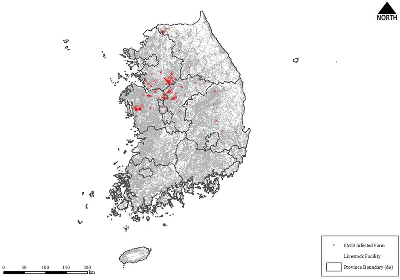
Spatial pattern of infected farms and livestock facilities.

According to Figure 1, the primary concentration of FMD incidents is identified in the Midwestern part of South Korea, especially in the border areas of Chungcheongnam-Do, Chungcheongbuk-Do, and Gyeonggi-Do. Here, “Do” points the top-level administrative boundary and is composed of several “Si–Gun–Gu” (SGG) areas. In summary, EMD that is also administrative boundary is geographically nested within SGG; SGG is then nested within Do. Along with the western SGGs in Chungcheongnam-Do and the northwestern SGGs of Ganwon-Do, two distinctive clusters of FMD incidents appeared.

The spatial distribution of livestock facilities looks much more crowded. It is hard to identify clear spatial distribution patterns of FMD incidents and livestock-related facilities by simply dotting the locations on the map, as shown in Figure 1. The kernel density maps of infected cases and facilities were created in Figure 2 and Figure 3, respectively. These figures visualize the overall outlines of the concentration on those geographic locations. For the generation of the kernel density maps, the Gaussian kernel method with the bandwidth of three kilometer was applied. Figure 2 presents the image demonstrating the geographic extent conspicuously, where FMD incidents are geographically concentrated. Also, Figure 3 shows the densely populated areas of livestock-related facilities in South Korea. The geographic information presented in both figures is difficult to obtain by plotting the locations on the map as shown in Figure 1.

Figure 2.

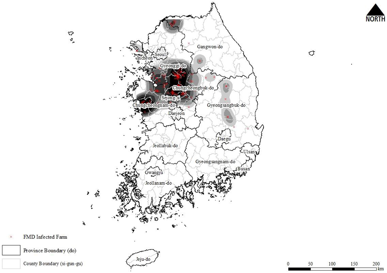
Spatial kernel density map: Foot-and-mouth disease cases.

Figure 3.

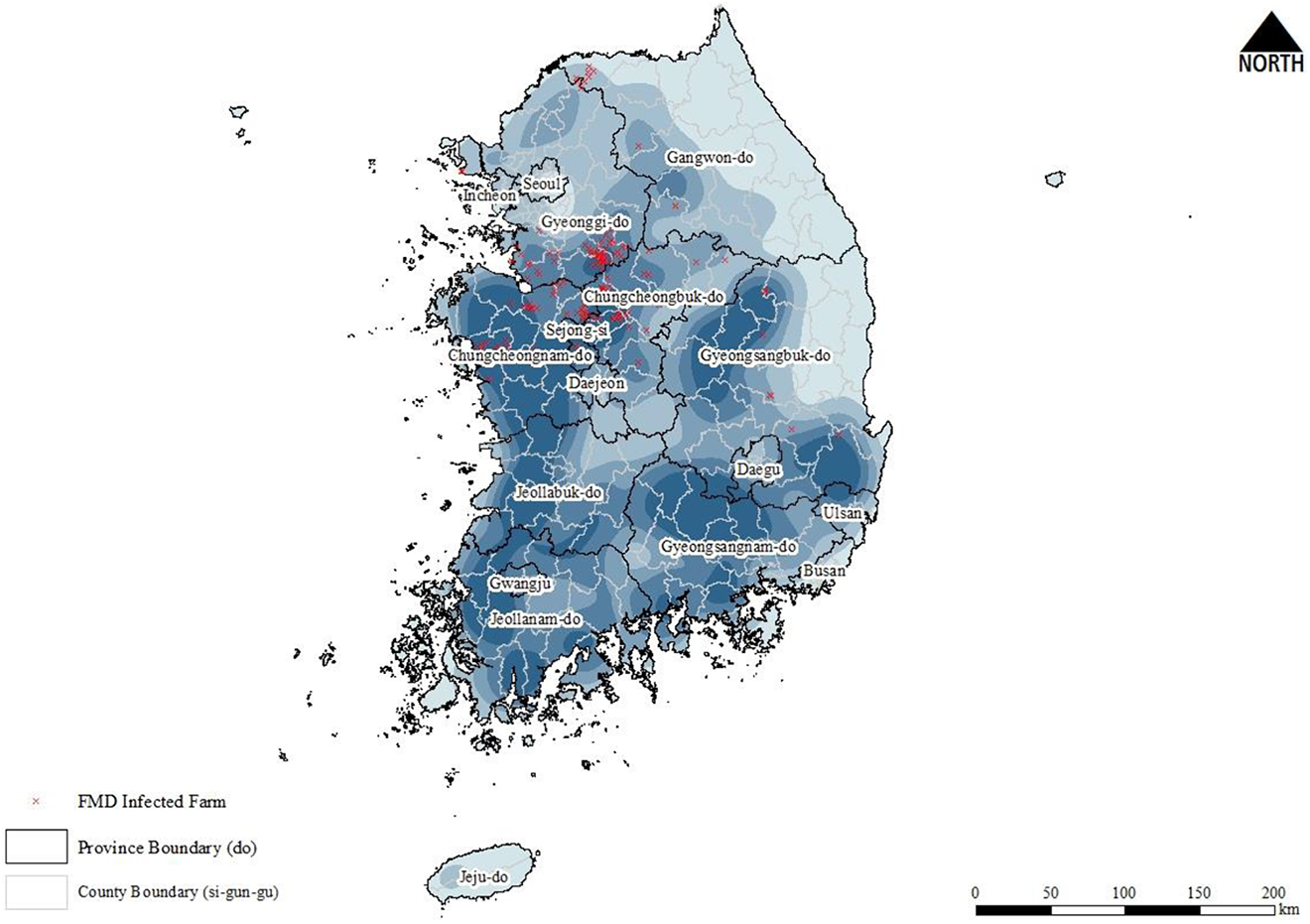
Spatial kernel density map: Livestock facilities.

Empirical Analysis and Results

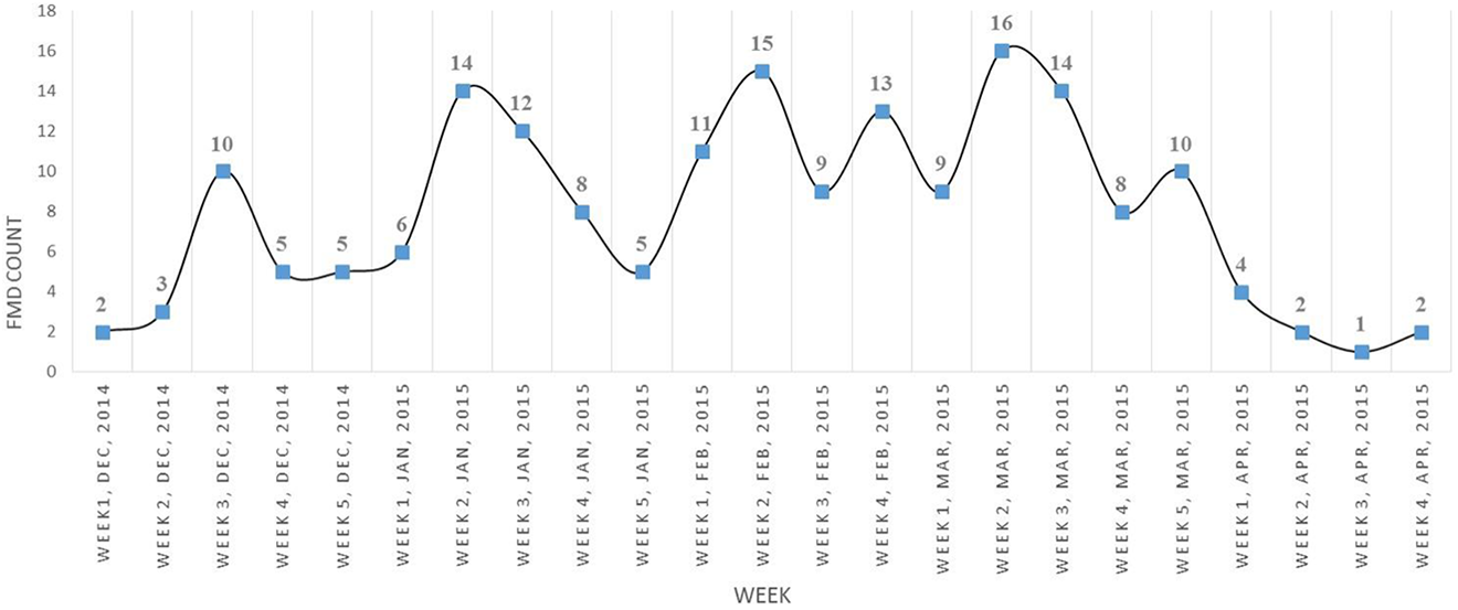
The empirical data set containing the information on 184 FMD outbreaks that occurred during five months were used for the calculation of ${STSC}_{i}$ . The first outbreak case was reported in a farm located in one EMD of Chungcheongbuk-Do on December 3, 2014; the last case was found in a farm located in Chungcheongnam-Do on April 28, 2015. No noticeable temporal pattern in the FMD occurrence was found; however, the occurrence frequency fluctuated repeatedly over time since the first week of December 2014 (see Figure 4). While the temporal cycle of a valid incubation period may be suspected as a positive factor for the frequency increase, the epidemic prevention activities may contribute to suppressing the spreading tendency and lead to the fluctuated temporal pattern.

Figure 4.

Fluctuated temporal variation in the foot-and-mouth disease occurrence.

For the empirical analysis, the probability of an event occurring in the vulnerable population is required to derive the expected count. It was set at 0.00046, which was approximated by dividing the number of infected cases by the number of facilities (=184/400,000). The parameters, $t w_c$ and $t_c$ , are set to be 0.01 and 21, respectively. It is based on the assumption that the incubation period for spreading FMD is twenty-one days (Hässig et al. 2015). If an FMD case is identified and another case is reported in twenty-one days later, it is supposed that the former barely affects the emergence of the latter. For the temporally weighted counts observed ( ${\tilde{O}}_{j}$ ) and the expected frequency (E_j ), a range of spatial scales from one kilometer to eighty-one kilometer by one kilometer was applied around each FMD occurrence location to compute ${STSC}_{i}$ . Among z values of ${STSC}_{i}$ generated in this manner, the spatial scale with the maximum z value is marked as a circle centered on the FMD-occurred facility location. The circle marked represents the overall geographic boundary of the first cluster, signifying the potentially highest-risk area in FMD occurrence. The cluster with the second maximum z value was also labeled as the second cluster if not overlapped geographically with the first cluster. The rule of no geographic overlap among clusters is applied to mark the third, the fourth, and the fifth as listed in descending order of the z value of ${STSC}_{i}$ .

Table 1 summarizes the significant analysis results on the five clusters identified with some information. Each cluster is labeled with SGG and EMD boundaries along with the incident date of the case and the geographic center of the cluster. Information on distance parameter (s_c), observed and expected counts (obs. and exp.), population at-risk, and relative risk (RR) is also provided. The observed count used for estimating RR is the sum of the temporal weights ( ${\tilde{O}}_{j}$ ). According to the result, all of the RR values are greater than one, indicating that the observed cases are found more than the expected in each cluster. The corresponding z values are much higher than the most conservative critical boundary in the normal distribution, which is 2.57 with the 1 percent significance level. This indicates that the high-risk areas found were not formed by a chance but highly probable, affected strongly by some factors contributing to the creation of each cluster.

However, note that the third and fourth clusters contain a small number of population at-risk facilities. In this instance, only one case plays a critical role in inflating RR. In the third cluster, only one case generated the RR value of 7.8, while the population at-risk is only 56. While somewhat smaller than the third one, the fourth cluster also shows a higher RR value due to only one case that occurred even when the population at-risk vulnerable to FMD infection is only 193 facilities. If a case is supposed to be rarely observed among the small number of vulnerable facilities, the emergence of only one case in that area may contribute to increasing RR much more than a case in densely populated areas. One possible inference is that some local factors in those areas may play a critical role in developing the third and fourth clusters.

As shown in Figure 5, considering that the two small clusters are geographically closest to the second cluster that demonstrates the most prevalent distribution of FMD incidents among others, it is supposed that the possibility of their aetiological associations with the second cluster is not entirely excludable. For example, Table 1 shows the highest z value in the second cluster indicating FMD incidents are most prevalent in that geographic extent. As shown in Figure 5, the third and the fourth clusters are geographically close to the second cluster. From this fact, it is inferred that frequent visits by many vehicles that stopped by FMD incident farms in the second cluster may transmit the virus to the farms in the third and/or the fourth clusters nearby. Also, facilities are not densely located in the third and the fourth clusters. This may hinder further geographic diffusion of the infectious disease since there exists no enough host population playing a role in transmitting the virus. Consequently, only small, fragmented clusters may be found in that locality. 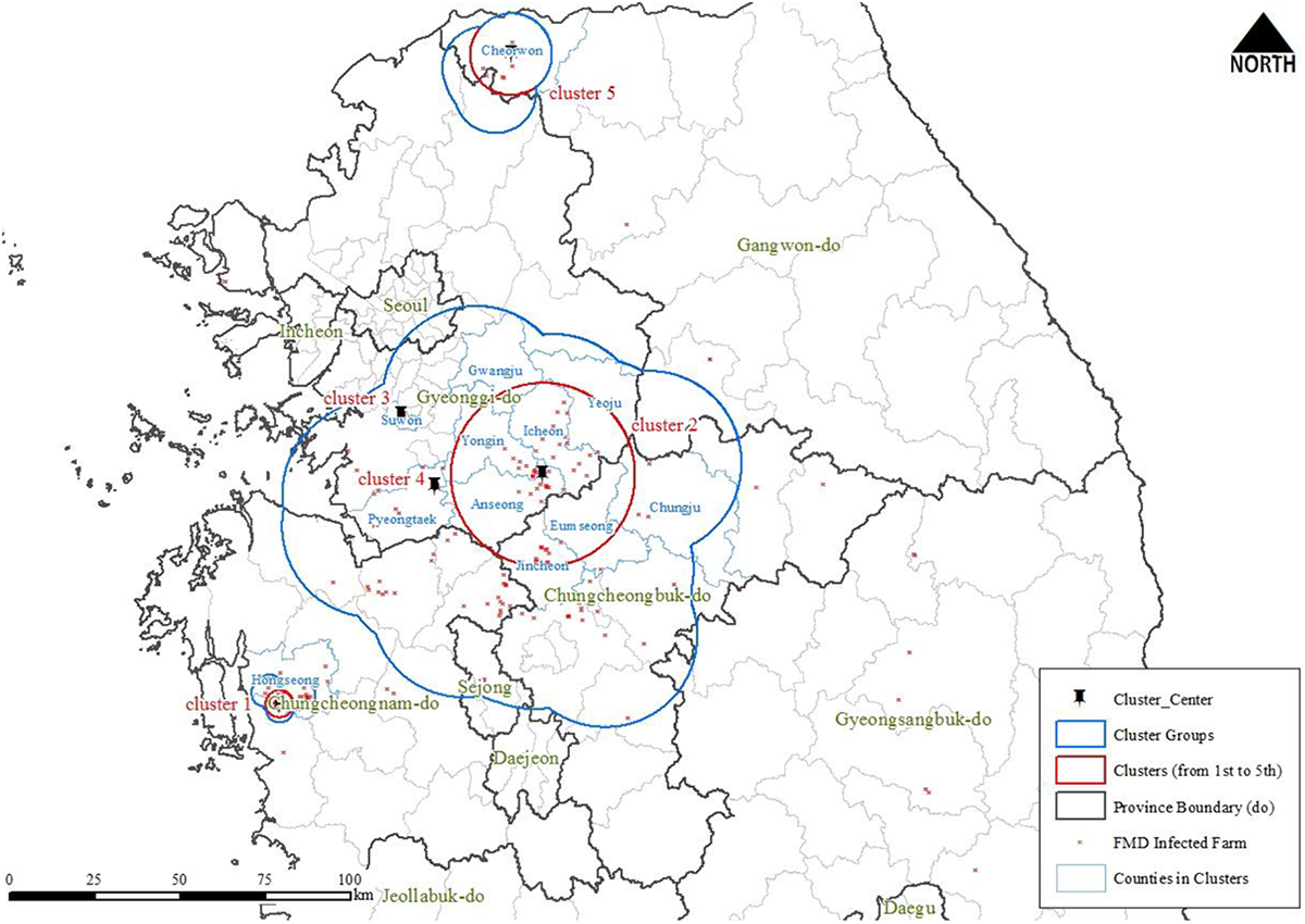The distance parameter showing the highest z value of ${STSC}_{i}$ is four kilometer for the first cluster. This is a relatively shorter local geographic extent. However, the second cluster shows the strongest clustering tendency with the highest z value among other clusters within the geographic extent of twenty-seven kilometer. The distance parameter values corresponding to the third and fourth clusters are only one kilometer, having a rather limited geographic extent. In the case of the fifth cluster, the parameter value is estimated to be twelve kilometer.

Figure 5.

Upper five clusters and geographic centroids.

Table 1.

Summary of Analytic Results.

Cluster	SGG	EMD	Incidence Date	Parameter (s_c)	Obs.	Exp.	Pop. at-Risk	RR	z Value
1	Hongseong	Cheonbuk	February 21, 2015	4,000	31	7.17	3,148	4.3	232.4
2	Anseong	Iljuk	January 22, 2015	27,000	58	32.37	14,213	1.8	148.3
3	Suwon	Seodun	March 13, 2015	1,000	1	0.13	56	7.8	117.5
4	Pyeongtaek	Songbuk	March 3, 2015	1,000	1	0.44	193	2.3	87.7
5	Cheorwon	Galmal	March 23, 2015	12,000	9	5.49	2,412	1.6	63.1

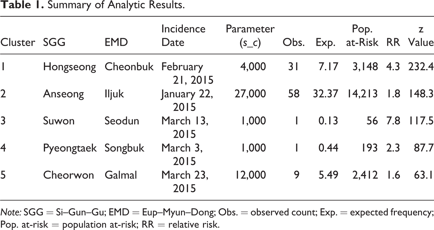
Note: SGG = Si–Gun–Gu; EMD = Eup–Myun–Dong; Obs. = observed count; Exp. = expected frequency; Pop. at-risk = population at-risk; RR = relative risk.

Figure 6 presented when the five clusters started to be formed. According to the figure, it seems that the first cluster was created after the second one had been formed. The third and fourth clusters look created almost simultaneously. The last cluster started to be generated around in the middle of the period that the fourth cluster covered. Therefore, we infer that the second cluster emerged firstly over an extensive geographic area and affected the formation of the first cluster. After that, the third and fourth clusters are marked geographically closer to the second cluster. The fifth cluster jumped out of the four clusters and is placed in subregions separated geographically, which are located in the northern territory of South Korea.

Figure 6.

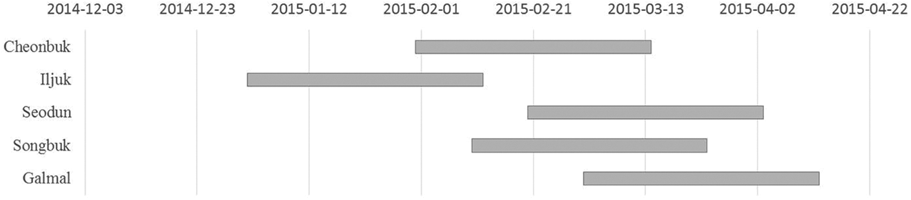
Temporal distribution of upper five clusters.

Figure 5 shows the five clusters pointing to the high-risk areas of FMD occurrence. On the map, the clusters are marked as circles. The circle center represents the location of FMD incident farms, and the size of each circle indicates the geographic extent of clusters. The first cluster is centered on Cheonbuk-Myun in Hongseong-Gun, Chungcheongnam-Do, covering a geographically limited extent with a radius of four kilometer. This may indicate a rather strong local interaction among nearby farms. That is, frequent visits to nearby farms via livestock movement vehicles and veterinarian inspection personnel are suspected of contributing to generating the locally elevated risk. The second cluster most highlighted in the map stretches the geographic extent to several SGGs throughout Chungcheongnam-Do, Chungcheongbuk-Do, and Gyeonggi-Do in the span of twenty-seven kilometer. The center of the second cluster is located in Iljuk-Myun of Anseong-Gun, Gyeonggi-Do, where livestock-related facilities are densely populated. In South Korea, it is noted that intensive and battery farming in those local areas with a high farm density is attributed to be one of the critical causes diffusing contagious animal diseases rapidly. Especially, the second cluster with the largest geographic extent is located over the highest farm density region in South Korea.

At first glance at the map in Figures 2 and 3, the FMD incident locations and the facilities show similar spatial distribution patterns. That is, the more the facilities are located in a region, the more FMD incidents are likely to be found in that region. This indicates the density of facilities mirrors that of FMD cases. However, the large clumps of geographic concentration of FMD incidents in border areas of Chungcheongnam-Do, Chungcheongbuk-Do, and Gyeonggi-Do do not merely explain the spatial density distribution of population at-risk. In calculating ${STSC}_{i}$ , the population at-risk vulnerable to FMD infection is accounted for in the expected count, and thus, the clusters showing the high z values are not merely due to the density of facilities. There may exist other factors suspected to contribute to generating a spatial clustering tendency in addition to the density of facilities.

The centers of the third and fourth clusters are found, respectively, in Seodun-Dong of Suwon-Si and Songbuk-Dong of Pyeongtaek-Si, both located within Gyeonggi-Do, while not clearly showing themselves on the map due to the small cluster size (one kilometer). The last cluster is identified in Galmal-Eup of Cheorwon-Gun, Gangwon-Do with a radius of twelve kilometer.

In addition to clusters, cluster groups are drawn as a blue line in Figure 5. Here, a cluster group comprises a couple of subclusters overlapped geographically with the main cluster. In the figure, for example, the first cluster (cluster 1) around Hongseong-Gun presented in the red circle is geographically overlapped with other nearby clusters with lower z values. The red-lined cluster 1 is the main cluster, while the other geographically overlapped ones are subclusters. The cluster group is identified as a simple aggregation of these clusters. Within a cluster group, the main cluster with the highest z value is overlapped geographically with nearby subclusters with lower z values, while not overlapped with clusters in other cluster groups. Because subclusters in a nested cluster group are not geographically overlapped with the subclusters in other cluster groups, no geographic overlap is permitted among cluster groups. In the case of the third and fourth clusters, additional subclusters were not identified. This may be because the size of the clusters is too small (one kilometer). Instead, the third and fourth clusters are completely nested within the cluster group of the first cluster. Finally, it seems that the cluster group containing the fifth cluster was created independently from the former cluster groups, which are geographically separated.

Model Evaluation

This study conducted a model evaluation process to demonstrate how STSC could outperform this type of research. First, a Monte Carlo simulation that creates an empirical distribution of the STSC test was carried out and compared to the distribution of SC and STSC. The Monte Carlo simulation was conducted for the 184 disease cases that were randomly assigned to 400,000 farms (population at-risk) to calculate SC and STSC. Repeating 10,000 times, the empirical distribution results of both SC and STSC were obtained, as shown in Figure 7. The proportion in the study area that has had FMD occurrence is very small as 0.00046, and hence, the Poisson λ (= 0.0845) will not follow a normal distribution as expected, resulting in a skewed distribution with the Monte Carlo simulation. We do not assume that this test holds a null hypothesis of equal risk of FMD among facilities because of the existing occurrence frequencies; instead, we intended to compare SC and STSC under the assumption that the normal approximation of z[STSC] will be valid if the assumption that z[SC] of Waller and Lawson is normal holds. According to the simulated results, both SC and STSC presented similar distributions while both statistics are skewed to the left side as expected. However, note that the min/max values of simulated z[SC] and z[STSC] are −3.59/4.71 and −3.65/3.77, respectively. Also, the mean values correspond to −0.93 and −1.25, while the variances correspond to 0.65 and 0.63, respectively, indicating both z-scores are skewed to the left side. This first test concludes that STSC will still be valid to hold the normal distribution assumption if SC holds a normal distribution because both distributions are similar for this Korean case.

Figure 7.

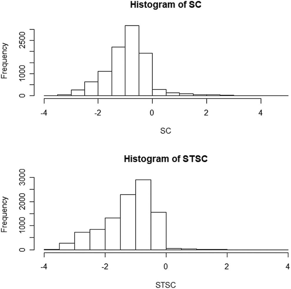
The empirical distribution of score statistic and spatiotemporal score statistic obtained from Monte Carlo simulations.

Second, to understand the null hypothesis of no spatiotemporal clustering, a statistical power analysis to estimate the number of rejecting the null hypothesis applied in the scenarios of elevated RR as conducted in Tango (1995) and Rogerson (1999). The elevated RR scenarios could test whether spatial clusters of the disease event exist. According to the SC definition that does not involve the time component, it is expected to reveal higher disease occurrences in an area than the STSC approach, resulting in overestimation of disease occurrence. Referring to Rogerson (1999), the elevated RR scenarios are conducted as follows: (1) on a hypothetical region, m locations were randomly distributed, where the population was assigned using the log-normal distribution. The study area is about 100,000 km². If the study area is transformed to a rectangle as a hypothetical region used for simulation, one side length is about 316 km. The mean and variance of the log-normal random variable were set to 4.6 and 0.5, respectively. Based on 400,000 farms and 184 cases that were located in 3,470 units of analysis (called Dong) comprising Provinces in the real area, but for simulation purpose, 3,470 units was reduced to 100 locations where population and other parameters were adjusted as such. Under the condition of RR = 3, the mean of 4.6 in the log-normal generated 184 cases approximately; (2) for a selected location, the elevated RR values greater than the regional background risk of RR that is equal to 1 were assigned. The RR values in the other locations decrease when applying the distance decay effect as in equation (2); (3) using RR and the population information in each location, n FMD cases were assigned. The temporal positions among the FMD cases were confined to five days and the temporal decay was applied as shown in equation (5), where the elevated RR scenarios hold valid; and (4) after n cases were assigned through steps above, the test statistic was calculated, repeating 10,000 times.

The statistical power of the test statistic was estimated as the number of rejecting the null hypothesis of no spatiotemporal clustering. The number was adjusted as divided by 10,000. This was applied repeatedly to the various RR scenarios ranging from 1.5 to 15. Figure 8 summarizes the test results with a range of RR scenarios. The labels of z1_0.1, z1_0.05, and z1_0.01 show the average rates of rejecting the null hypothesis based on 10,000 simulations when SC is applied for a range of RR values under α = .1, .05, and .01, respectively. Likewise, z2_0.1, z2_0.05, and z2_0.01 demonstrates the rejection rates when STSC is applied in the same experimental settings. Overall, the rejection rates of SC are higher than those of STSC. For a range of lower RR values, this pattern is apparent. As RR increases, the rejection rates are converging for all the significance levels. This indicates that SC may possibly overreject the null hypothesis than STSC in the low RR scenarios, and consequently, the Type-I error of SC may be much higher than that of STSC. In the scenarios of higher risk, both SC and STSC demonstrated higher rates of rejecting the null spatiotemporal pattern while SC shows higher rejection rates consistently.

Figure 8.

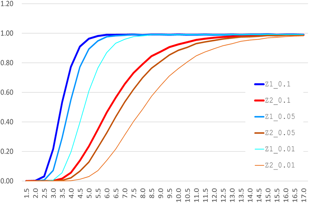
Simulation results for testing the statistical power of score statistic and spatiotemporal score statistic.

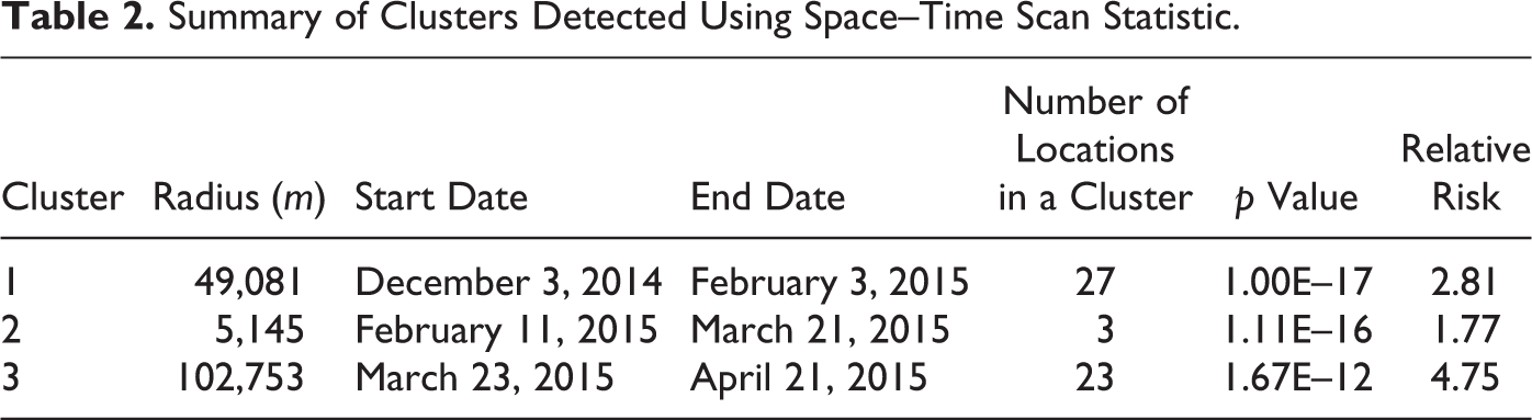
Third, for a comparison purpose, a spatiotemporal cluster analysis was conducted by applying a spatiotemporal scan statistic (STSS) approach. We used a space–time permutation probability model in SaTScan software. The size of the spatial and temporal scanning windows was limited to 50 percent of the total population at-risk. Table 2 and Figure 9 show the analytic result of STSS. The first was identified with twenty-seven cases and RR = 2.81. The spatial range of the cluster was about forty-nine kilometer for a temporal range of about two months, as demonstrated in Figure 9. The second cluster detected was geographically restricted with three cases and RR = 1.77 for a temporal range of about forty days. The third cluster with twenty-three cases and RR = 4.75 covered a vast geographic area within less than one-month period. The results show that all the clusters were statistically very significant with p values close to zero. Comparing Figure 5, the first cluster detected using STSS somewhat shifted toward southeast direction, while the spatial range of the second cluster is almost identical to the second cluster in Figure 5. The third cluster in Figure 9 covers a vast geographic range close to the first cluster. This is quite different in the geographic location and range from the third cluster applied with STSC as shown in Figure 5; the STSC’s third cluster location was considerably separated from the first cluster and situated in the northern part of the study region and the geographic range of the cluster was rather limited. While the STSC clusters demonstrated similar geographic locations and ranges to the STSS approach except the third one, STSC has a spatiotemporal merit in the cluster detection, which is more useful for policy application.

Figure 9.

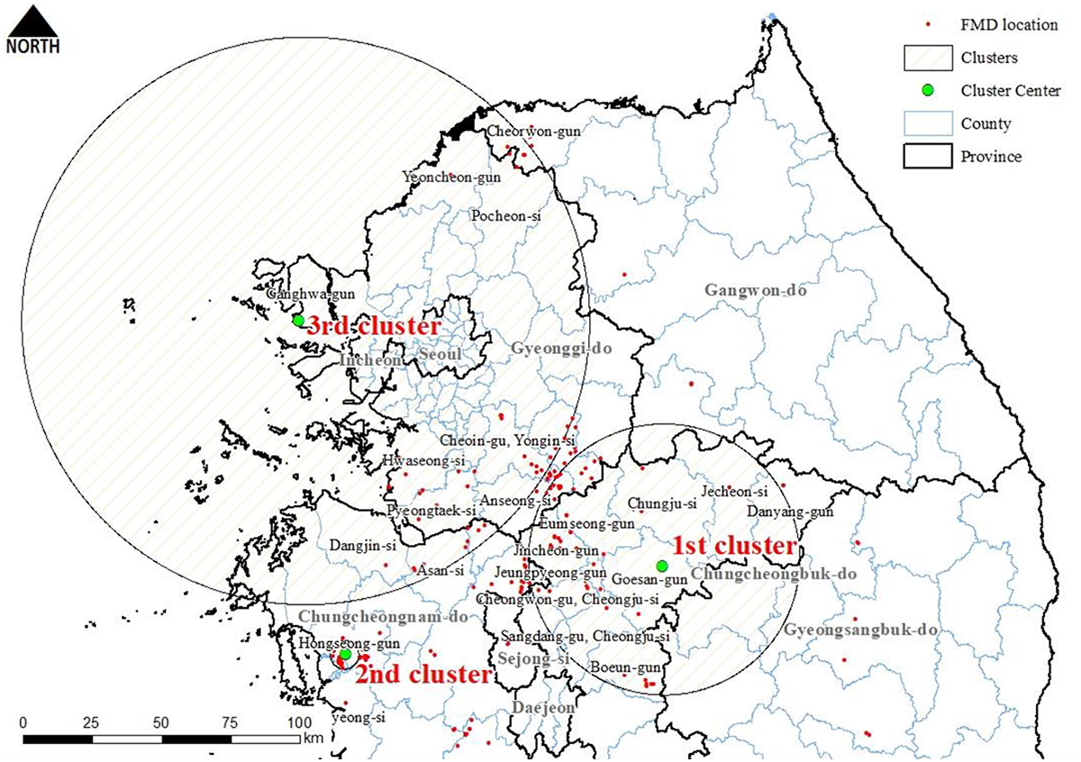
Geographic locations and the range of detected clusters using a space–time scan statistic.

Table 2.

Summary of Clusters Detected Using Space–Time Scan Statistic.

Cluster	Radius (m)	Start Date	End Date	Number of Locations in a Cluster	p Value	Relative Risk
1	49,081	December 3, 2014	February 3, 2015	27	1.00E–17	2.81
2	5,145	February 11, 2015	March 21, 2015	3	1.11E–16	1.77
3	102,753	March 23, 2015	April 21, 2015	23	1.67E–12	4.75

Conclusions and Discussion

This study suggested the use of STSC extended from the original SC to identify high-risk areas. High-risk areas where FMD occurrences were concentrated refer to the spatial clusters with the maximum local z values of ${STSC}_{i}$ . While the spatial clusters were not geographically overlapped, the temporal periods of the clustering process were overlapped in the analysis process.

It looks that some influential permanent factors may affect the formation of spatial clusters as potential high-risk areas. As such, an additional epidemic is concerned with persisting around those localities in the future. Among others, the contact relationship among facilities created by vehicle movements could be critical in transmitting the infectious disease (Kerkhove et al. 2009). Based on this supposition, if a vehicle visited one facility infected and visits another facility, for example, within the incubation period such as twenty-one days, the contact relationship may comprise one piece of pathways in transmitting the virus. If FMD-occurred facilities in the clusters are interconnected via frequent visits of vehicles, it is strongly believed that the vehicle movement could significantly generate the epidemic in a chain, playing a critical role in creating and extending the high-risk areas over a vast geographic range. As shown in Figure 5, frequent visits by the vehicles to facilities along with the high-density breeding environment in South Korea could accelerate the spread of disease, broadly expanding some marked spatial clusters of disease occurrence, especially in Gyeonggi-Do and Chungcheongnam-Do. If the visit of a livestock-related vehicle is assumed to be one of the major factors spreading the disease, measures of preventing and controlling the spread of the disease that include the banning rule of vehicles could not be effective in the early stage of the epidemic. Consequently, the disease may get into the first cluster (centered on Anseong-Gun) during the incubation period of the second cluster center. This may trigger the formation of the first cluster after that. Again, the fifth cluster was found in Cheorwon-Gun located in the northern part of South Korea after the third and fourth clusters were identified. The fifth cluster was quite far from the four clusters. This suggests additional inferential evidence that the vehicle movement may be a critical cause of the rapid spread of FMD nationwide during the study period.

Another factor affecting the creation of FMD clusters can be the requirement of installing burial sites around the FMD-occurred farms. The leachate leaked from the burial sites may increase the possibility of transmitting the virus to adjacent facilities, especially located in the highly dense environment of breeding. Therefore, the burial sites need to be cautiously determined and persistently monitored to cope with the potential threats generated from the leakage of leachate and the subsequent local spread.

Based on the empirical analysis results, some policy suggestions and further discussing points for preventing and controlling the epidemic of FMD are addressed as follows: firstly, it is useful to establish the substantial and collaborative governance system in preventing and controlling epidemics among adjacent SGGs suffering from the prevalence of FMD. Although the local government at the SGG level is primarily responsible for preventing the epidemic in the early stage, the nationwide spread in a short period implies that the SGG-level activities may not be practically effective for epidemic prevention and control. Thus, mid- and long-term strategic plans to strengthen the cooperation system among SGGs need to be arranged urgently. Secondly, major quarantine zones need to be designated as another potential measure to implement the prevention and control strategies. By identifying roads connecting the clusters where numerous livestock-related vehicles are frequently passing through, this can be achievable. The analysis results marking the center locations and the geographic extent of the spatial clusters can be worth utilizing some clue information in designating quarantine zones. Thirdly, the foothold facilities can be selectively located at important positions on the road network where the livestock-related vehicles frequently path through fumigating the virus. That is, major nodes may be pinpointed, passing through the road network concentrated in major quarantine zones within the identified spatial clusters. Indeed, information on the spatial clusters may be useful in implementing various policy tools.

A future study aiding to prevent and control the epidemic of FMD can be developed using the log data of vehicle visits to facilities. To do so, the log data of KAHIS need to be properly maintained and updated in real time since the data allow potential disease transmission paths to be monitored. Once recording the pathways through which the vehicles visited the FMD-positive farms within the incubation period, the potential routes of spreading the infection can be effectively identified. Also, burial sites should be practically utilized as local foci that play the potential sources of infection and applied to STSC _i . Additional analysis utilizing the burial sites as local foci can shed more light on figuring out the potential aetiologic role of burial sites in detecting spatial clusters. Finally, while this study briefly compared both STSC and STSS approaches, which provide a benefit of understanding a proper null hypothesis and the related statistical model that has not been substantially discussed, rigorous verification of whether this STSC type method outperforms the exiting space-time methods should be pursued in-depth. Even though the practical benefit of identifying a spatial pattern using time component and has a potential to be developed for a dynamic model (Keeling et al. 2001), this present study can be ill-posed from a statistical viewpoint because the score functions may lose asymptotic normality property in a standard model due to the issue in the number of observation itself. That is, the normality assumption is not satisfied primarily since the number of observations is too small relative to the population (the entire premises), by collecting more data, our approach can resolve the normality issue. It is also worth noting that this issue is possibly associated with a compound process of summing random time intervals, and hence, a rigorous stepwise process that includes statistical concepts and technical details requires as a next trial.

Footnotes

Authors’ Note

Any opinions, findings, conclusions, or recommendations in this article are those of the authors and do not necessarily reflect the views of the Korea Institute of Planning and Evaluation for Technology in Food, Agriculture, Forestry and Fisheries and the Ministry of Agriculture, Food and Rural Affairs. Also, the authors sincerely appreciate precicous comments of three anonimous reviewers, which improved the article significantly.

Declaration of Conflicting Interests

The author(s) declared no potential conflicts of interest with respect to the research, authorship, and/or publication of this article.

Funding

The author(s) disclosed receipt of the following financial support for the research, authorship, and/or publication of this article: This research was supported by the Korea Institute of Planning and Evaluation for Technology in Food, Agriculture, Forestry and Fisheries under contract number C1012360-01-01 through the Animal Disease Management Technology Development Program that was funded by the Ministry of Agriculture, Food and Rural Affairs.

ORCID iDs

Son-Il Pak

JiYoung Park

References

Berke

Beilage

E. G.

. 2003. “Spatial Relative Risk Mapping of Pseudorabies-seropositive Pig Herds in an Animal-dense Region.” Journal of Veterinary Medicine B 50:322–25.

Bessell

P. R.

Shaw

D. J.

Savill

N. J.

Woolhouse

M. E.

. 2010. “Statistical Modeling of Holding Level Susceptibility to Infection during the 2001 Foot and Mouth Disease in Great Britain.” International Journal of Infectious Diseases 14:e210–15.

Calistri

Iannetti

Atzeni

Di Bella

Schembri

Giovannini

. 2013. “Risk Factors for the Persistence of Bovine Brucellosis in Sicily from 2008 to 2010.” Preventive Veterinary Medicine 110:329–34.

Chhetri

B. K.

Perez

A. M.

. 2010. “Factors Associated with Spatial Clustering of Foot-and-mouth Disease in Nepal.” Tropical Animal Health and Production 42:1441–49.

Ekong

P. S.

Ducheyne

Carpenter

E. E.

Owolodun

O. A.

Oladokun

A. T.

Lombin

L. H.

Berkvens

. 2012. “Spatio-temporal Epidemiology of Highly Pathogenic Avian Influenza (H5N1) Outbreaks in Nigeria, 2006–2008.” Preventive Veterinary Medicine 103:170–77.

Ersbøll

A. K.

Ersbøll

B. K.

. 2009. “Simulation of the K-function in the Analysis of Spatial Clustering for Non-randomly Distributed Locations-exemplified by Bovine Virus Diarrhea Virus (BVDV) Infection in Denmark.” Preventive Veterinary Medicine 91:64–71.

Firestone

S. M.

Christley

R. M.

Ward

M. P.

Dhand

N. K.

. 2012. “Adding the Spatial Dimension to the Social Network Analysis of an Epidemic: Investigation of the 2007 Outbreak of Equine Influenza in Australia.” Preventive Veterinary Medicine 106:123–35.

Hässig

Meier

A. B.

Braun

Hässig

Schmidt

Lewis

. 2015. “Cattle Movement as a Risk Factor for Epidemics.” SAT (Schweizer Archiv für Tierheilkunde) 157:441–48.

Jacquez

G. M.

1996. “A k Nearest Neighbour Test for Space-time Interaction.” Statistics in Medicine 15:1935–49.

10.

Jacquez

G. M.

2008. “Spatial Cluster Analysis.” In The Handbook of Geographic Information Science, edited by Wilson

J. P.

Fotheringham

A. S.

, 395–416. Malden, MA: Blackwell.

11.

Keeling

M. J.

2005. “Models of Foot-and-mouth Disease.” Proceedings of the Royal Society of London B 272:1195–202.

12.

Keeling

M. J.

Woolhouse

M. E. J.

Shaw

D. J.

Matthews

Chase-Topping

Haydon

D. T.

Cornell

S. J.

Kappey

Wilesmith

Grenfell

B. T.

. 2001. “Dynamics of the 2001 UK Foot and Mouth Epidemic: Stochastic Dispersal in a Heterogeneous Landscape.” Science 294 (5543): 813–17. doi: 10.1126/science.1065973.

13.

Kerkhove

M. D. V.

Vong

Guitian

Holl

Mangtani

San

Ghani

A. C.

. 2009. “Poultry Movement Networks in Cambodia: Implications for Surveillance and Control of Highly Pathogenic Avian Influenza (HPAI/H5N1).” Vaccine 27:6345–52.

14.

Kulldorff

1995. “Spatial Disease Clusters: Detection and Inference.” Statistics in Medicine 14:799–810.

15.

Kulldorff

1997. “A Spatial Scan Statistic.” Communication in Statistics—Theory and Methods 26:1481–96.

16.

Lawson

A. B.

1993. “On the Analysis of Mortality Events Associated with a Prespecified Fixed Point.” Journal of the Royal Statistical Society. Series A 156:363–77.

17.

Lee

Park

J. Y.

Gordon

Moor II

J. E.

Richardson

H. W.

. 2012. “Estimating the State-by-state Economic Impacts of a Foot-and-mouth Disease Attack.” International Regional Science Review 35:26–47.

18.

Maheswaran

Staines

. 1997. “Cancer Clusters and Their Origins.” Chemistry and Industry 7:254–56.

19.

Martinez-Lopez

Perez

A. M.

Sanchez-Vizcaino

A. M.

. 2009. “Combined Application of Social Network and Cluster Detection Analyses for Temporal-spatial Characterization of Animal Movements in Salamanca, Spain.” Preventive Veterinary Medicine 91:29–38.

20.

Menach

A. L.

Legrand

Grais

R. F.

Viboud

Valleron

A. J.

Flahault

. 2005. “Modeling Spatial and Temporal Transmission of Foot-and-mouth Disease in France: Identification of High-risk Areas.” Veterinary Research 36:699–712.

21.

Minh

P. Q.

Morris

R. S.

Schauer

Stevenson

Benschop

Nam

H. V.

Jackson

. 2009. “Spatio-temporal Epidemiology of Highly Pathogenic Avian Influenza Outbreaks in the Two Deltas of Vietnam during 2003–2007.” Preventive Veterinary Medicine 89:16–24.

22.

Neutra

R. R.

1990. “Counterpoint from a Cluster Buster.” American Journal of Epidemiology 132:1–8.

23.

Nogareda

Juberta

Kantzoura

Kouam

M. K.

Feidas

Theodoropoulos

. 2013. “Geographical Distribution Modelling for Eospora Caninum and Coxiella Burnetii Infections in Dairy Cattle Farms in Northeastern Spain.” Epidemiology and Infection 141:81–90.

24.

Olsen

F. S.

Martuzzi

Elliott

. 1996. “Cluster Analysis and Disease Mapping—Why, When, and How? A Step by Step Guide.” British Medical Journal 313 (5): 863–66.

25.

Paul

Wongnarkpet

Gasqui

Poolkhet

Thongratsakul

Ducrot

Roger

. 2011. “Risk Factors for Highly Pathogenic Avian Influenza (HPAI) H5N1 Infection in Back Yard Chicken Farms, Thailand.” Acta Tropica 118:209–16.

26.

Perez

A. M.

Thurmond

M. C.

Grant

P. W.

Carpenter

T. E.

. 2005. “Use of the Scan Statistic on Disaggregated Province-based Data: Foot-and-mouth Disease in Iran.” Preventive Veterinary Medicine 71:197–207.

27.

Perez

A. M.

Ward

M. P.

Carpenter

T. E.

. 2004. “Control of Foot-and-mouth Disease Epidemic in Argentina.” Preventive Veterinary Medicine 65:217–26.

28.

Pfeiffer

D. U.

Minh

P. Q.

Martin

Epprecht

Otte

M. J.

. 2007. “An Analysis of the Spatial and Temporal Patterns of Highly Pathogenic Avian Influenza Occurrence in Vietnam Using National Surveillance Data.” The Veterinary Journal 174:302–09.

29.

Pfeiffer

D. U.

Robinson

R. P.

Stevenson

Stevens

K. B.

Rogers

D. J.

Clements

A. C. A.

. 2008. Spatial Analysis in Epidemiology. Oxford, UK: Oxford University Press.

30.

Pinto

A. A.

2004. “Foot-and-mouth Disease in Tropical Wildlife.” Annals of New York Academy of Science 1026:65–72.

31.

Premashthira

Salman

M. D.

Hill

A. E.

Reich

R. M.

Wagner

B. A.

. 2011. “Epidemiological Simulation Modeling and Spatial Analysis for Foot-and-mouth Disease Control Strategies: A Comprehensive Review.” Animal Health Research Reviews 12:225–34.

32.

Riley

2010. “Coping without Farm Location Data during a Foot-and-mouth Outbreak.” Proceedings of National Academy of Sciences of the United States of America 107:957–58.

33.

Rogerson

P. A.

1999. “The Detection of Clusters Using a Spatial Version of the Chi-square Goodness-of-fit Statistic.” Geographical Analysis 31 (1): 130–47.

34.

Rogerson

P. A.

2001. “A Statistical Method for the Detection of Geographical Clustering.” Geographical Analysis 33 (3): 215–27.

35.

Rogerson

P. A.

Yamada

. 2009. Statistical Detection and Surveillance of Geographic Clusters. Boca Raton, FL: CRC Press.

36.

Tango

1995. “A Class of Tests for Detecting ‘General’ and ‘Focused’ Clustering of Rare Diseases.” Statistics in Medicine 14 (21–22): 2323–34.

37.

Wakefield

J. C.

Kelsall

J. E.

Morris

S. E.

. 2000. “Clustering, Cluster Detection and Spatial Variation in Risk.” In Spatial Epidemiology—Methods and Applications, edited by Elliott

Wakefield

J. C.

Best

N. G.

Briggs

D. J.

, 128–52. Oxford, UK: Oxford University Press.

38.

Waller

L. A.

Gotway

C. A.

. 2004. Applied Spatial Statistics for Public Health Data. Hoboken, NJ: John Willey & Sons.

39.

Waller

L. A.

Wheeler

D. C.

Switchenko

J. M.

. 2016. “Focused Clustering: Statistical Analysis of Spatial Patterns of Disease around Putative Sources of Increased Risk.” In Handbook of Spatial Epidemiology, edited by Lawson

Banerjee

Hanining

Ugarte

, 449–75. Boca Raton, FL: CRC Press.

40.

Wilesmith

J. W.

Stevenson

M. A.

King

C. B.

Morris

R. S.

. 2003. “Spatio-temporal Epidemiology of Foot-and-mouth Disease in Two Counties of Great Britain in 2001.” Preventive Veterinary Medicine 61:157–70.

41.

Zhang

Chen

Davies

T. M.

Vaillancourt

J. P.

. 2012. “Risk Signals of an Influenza Pandemic Caused by Highly Pathogenic Avian Influenza Subtype H5N1: Spatio-temporal Perspective.” The Veterinary Journal 192:417–21.