
Abstract
In this paper, we introduce a new way of modeling spatial regimes using smooth transitions. We propose an autoregressive spatial lag model where a logistic function captures structural variation in the spatial lag parameter. In the regime-switching spatial lag model with smooth transitions, the effect of the spatial neighbors depends on the transition variable that governs the regime switch. An LM test for detecting nonlinearity is derived, and a simulation study, where the properties of the test are investigated, is conducted. The test shows good power in relatively small samples with moderate deviation from linearity. An empirical application is included, where data on median house prices from the Boston area is used to explore the spatial dependence between census tracts. A smooth shift between regimes governed by the variable property tax rate is found. The smooth spatial lag model performs slightly better than the regular spatial lag model in terms of model fit and capturing spatial dependence.
Introduction
Geographical data generally possess spatial effects, meaning that observations in neighboring locations influence each other more than those farther apart. Taking these effects into account is of great importance in applied statistical work, as it will influence results used for predictions and the implementation and evaluation of policies. Spatial dependence is one of two types of spatial effects found in cross-sectional data. It can be described as a functional relationship between what happens at different points in space and is typically modeled using spatial linear regression models (Anselin 1988b). The other type of effect is spatial heterogeneity, which occurs if the effects of space are structurally different for different locations. Spatial heterogeneity can manifest through problems such as heteroscedasticity, random coefficient variation, and switching regressions. The latter is used when the heterogeneity is of a form that categorizes the observations into different regimes. The regimes may possess different regression coefficients, weight matrices, or explanatory variables. In addition to spatial heterogeneity, switching regressions can also account for spatial dependence (Anselin 1988b). In this paper, we introduce a model that deals with systematic variation in the parameter measuring the average level of influence spatial neighbors have on the dependent variable. By letting one of the exogenous variables determine the switch, we create a new type of spatial regimes model in which the effects of neighbors differ and where observations are allowed to exist between regimes.
The most common choices for modeling spatial dependence are the spatial lag and spatial error models. The former includes a spatially lagged dependent variable in the model, while the latter accounts for spatial dependence in the error terms. The theory of spatial linear regression models is well developed in the literature, where maximum likelihood is most frequently used for testing and estimating the parameters of the models (Anselin 1988a, Anselin and Rey 1991; LeSage and Pace 2009). Alternative approaches include GMM and IV estimation, which have been put forth and developed by Kelejian and Prucha (1999), Kelejian, Prucha, and Yuzefovich (2004), Kelejian and Prucha (2010), Lin and Lee (2010), and Saavedra (2003), among others.
Spatial regimes refer to distinct patterns or characteristics observed within specific geographic areas. Examples of spatial regimes include rural and urban areas, which generally exhibit substantial differences in population density, infrastructure, and socioeconomic factors, leading to spatial heterogeneity. Correctly identifying regimes and getting a deeper understanding of the effect of spatial neighbors is crucial in many applications. For example, it can help in developing targeted policies to promote economic growth in certain areas (see Andreano, Benedetti, and Postiglione 2017) or to find crime patterns that can guide crime prevention initiatives. It is further important in health geography, where a proper understanding of the effect of spatial neighbors can help with resource allocation and healthcare planning, as well as in climate studies when there is a need to develop region-specific adaptation strategies to climate change. Some recent applications covering these, and similar scenarios include Graif and Sampson (2009), Auteri et al. (2019), Vandenbulcke et al. (2011), and Billé, Salvioni, and Benedetti (2018).
The traditional way of modeling spatial regimes is to identify the different regimes a priori and then estimate the model parameters (Anselin 1988b). Structural instability in a standard spatial lag model can be detected with a Chow test, and regimes can subsequently be identified from exploratory analyses. Although spatial regimes models account for structural instability in the regression parameters, they typically assume constant spatial lag parameters across regimes. Different weight matrices can be estimated, although it requires knowledge of how to allocate observations into regimes. In many applications, the observations cannot be easily categorized into regimes such as “south/north,” “east/west,” or “urban/rural.” Furthermore, the influence of neighboring locations may be structurally different across space, something that can be caused by phenomena such as localized effects or contextual factors. For example, in certain ecological studies, the influence of neighboring habitats on species' abundance might vary depending on the specific characteristics of each location. In social science studies, the impact of neighboring districts might differ depending on local socioeconomic conditions or cultural factors. In these situations, we propose to use a spatial lag model with smoothly varying lag parameters. The proposed model drives the transition between regimes by a theoretically justified transition variable likely to influence the regime switch. Our main contribution is to present a test for detecting smooth transition type nonlinearity in the spatial lag parameter in a spatial regression model. Suppose the null hypothesis of linearity is rejected for a certain variable. In that case, that variable can be used in estimating a spatial regimes model with systematic variation in the influence of neighbors. Choosing the appropriate transition variable can be done in several ways and depends on the objective of the analysis. In the smooth transition literature, it is common practice to choose one of the explanatory variables in the model, based on theory, and/or test several variables and choose the one with the lowest p-value (Teräsvirta 1994; Teräsvirta, van Dijk, and Franses 2002). One benefit of the approach we suggest is that it does not require a priori categorization into regimes, as this is done in estimating the model. The switching point and speed at which the observations move between regimes are also estimated, which makes the model more flexible than a traditional spatial two-regime model.
The standard smooth transition autoregressive (STAR) model developed for time series data extends the threshold model that separates a process into two regimes to one where the switch between regimes is smooth. The STAR framework has received much attention and is well established in the non-linear time series literature (Luukkonen, Saikkonen, and Teräsvirta 1988; Teräsvirta 1994; Teräsvirta, van Dijk, and Franses 2002). Previous work that combines spatial analysis and STAR models include that of Pede, Florax, and Lambert (2014), which introduces a spatial STAR model that accounts for STAR-type nonlinearity in the exogenous variables but assumes a non-varying spatial lag parameter. Like these authors, we include a logistic transition function in the model but place it with the spatial lag parameter. This approach enables the interpretation that the effect of spatial neighbors depends on the transition variable that governs the regime switch. The resulting smooth spatial lag model can be seen as having two extreme regimes that occur when the transition function is zero or one. Observations with values in-between are seen as being in transition between regimes. For example, if we consider modeling crime rate in a certain area where there is no obvious classification of regimes, a socioeconomic variable such as education level could be a candidate transition variable. The average influence neighboring locations have on crime levels would be structurally different in the two regimes, and which regime a given location belongs to would depend on the education level. If the transition variable is estimated to be a low number, many locations will be in transition between regimes. Although this model focuses specifically on the structural difference in the lag parameter, it could be extended to include varying coefficients for the exogenous regressors. It could further be extended to include spatially lagged exogenous variables, thus encompassing a spatial Durbin model.
To test for linearity, we derive an LM-type test based on that of Luukkonen, Saikkonen, and Teräsvirta (1988). A Monte Carlo study shows that the small sample properties for the test are good, in terms of size and power, for moderate sample sizes with non-negligible differences between regimes.We further demonstrate the practical use of the model in an empirical application, estimating median house prices using the Boston house price data available from the R package SpData. We find a smooth shift from a regime with a weak average influence of neighbors on house prices to one with a strong influence governed by property tax rates.
The remainder of the paper is organized as follows. In the next section, we present the smooth spatial lag model, how to estimate it, and derive a nonlinearity test. Following this, a Monte Carlo experiment investigating the small sample properties of the test, is conducted. Subsequently, we demonstrate the use of the model in a empirical application. The paper concludes with a summary of the findings.
The Smooth Spatial Lag Model
We start this section by introducing and defining the smooth spatial lag model, followed by a description of how to estimate the model and how to test for nonlinearities.
One of the most common ways of modeling spatial dependence in cross-sectional data sampled at one time point is through the mixed regressive-spatial autoregressive model. This model is represented as


Estimation
Estimation of the spatial lag model can be done in several ways. As the OLS estimator is inconsistent in the presence of a spatial weight matrix, much of the early work has focused on a maximum likelihood approach. Maximum likelihood estimators for the spatial lag model have been derived and applied by Anselin (1988a), amongst others. Their results can easily be extended to the smooth spatial lag model. The analytical maximum likelihood estimators for β and σ2 in (4) are


The concentrated log-likelihood function follows as

Using the simplification proposed by Ord (1975), the concentrated log-likelihood function can be expressed as

LM Test for Nonlinearity
We use a Lagrange multiplier test to test the smooth spatial lag against a regular spatial lag. When testing for smooth transitions in a time series setting, the standard procedure is to use a first-order Taylor approximation of the transition function, around γ = 0. This is done to avoid the problem of unidentified nuisance parameters under the null hypothesis (Teräsvirta, Tjøstheim, and Granger (2010)). A Taylor approximation of the transition function around γ = 0 is given by
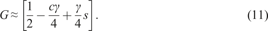
Substituting (11) for (4) yields the auxiliary regression model
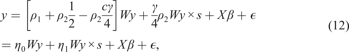


The LM test for η1 = 0 is a straightforward extension of the test for ρ = 0 in (1), derived by Anselin (1988 b), and closely follows the tests presented by Pede, Florax, and Lambert (2014). The derivations of the test are presented in the Appendix.
Monte Carlo Simulations
To investigate the small sample properties of the derived LM test, we perform a Monte Carlo experiment where size and power simulations are conducted.
The simulation design is set up to resemble that of Pede, Florax, and Lambert (2014) as closely as possible. As such, it follows standard Monte Carlo practices for evaluating tests in spatial econometrics. By their design, three types of weight matrices are used in the experiments. Firstly, we consider a row standardized weight matrix based on the k nearest neighbors of each spatial unit. The number of neighbors k is defined as the square root of the sample size n. Secondly, we consider a weight matrix based on the inverse of the Euclidean distance of the k nearest neighbors. These matrices are based on x, y coordinates simulated from a U(0, 1) distribution. Finally, a queens contiguity weight matrix is considered, set up as a regular n × n grid. The three matrices are row-standardized to have the sum of each row equal one. For the distance-based weight matrices, we thus have a random placement based on simulated coordinates, and for the queens matrix, we have a regular lattice, meaning that each location has three, five, or eight neighbors. These weight matrices are considered known in the experiment. The spatial lag model with smooth transitions is defined as

Empirical Size of the LM Test for Linearity, for Three Types of Weight Matrices.

Notes: A 95% confidence interval for the rejection proportion p is given by 0.0425 < p < 0.05975. Values that fall within the interval are marked with an asterisk.
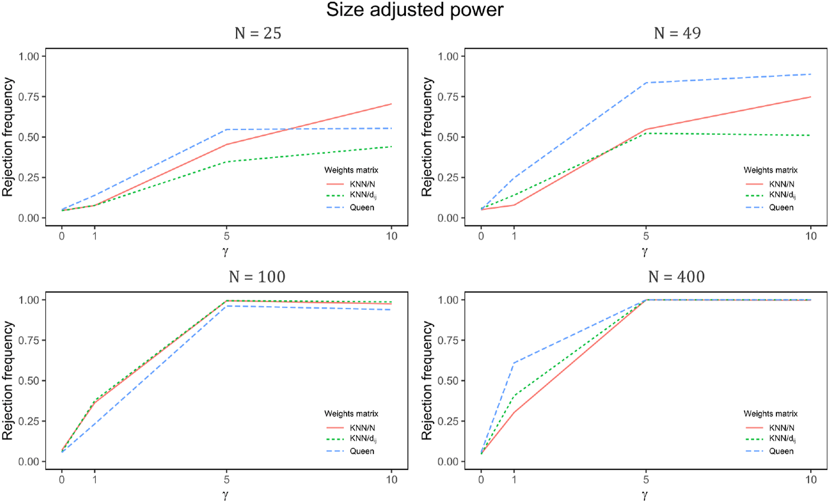
Size adjusted power when ρ1 = 0.1 and ρ2 = 0.8.
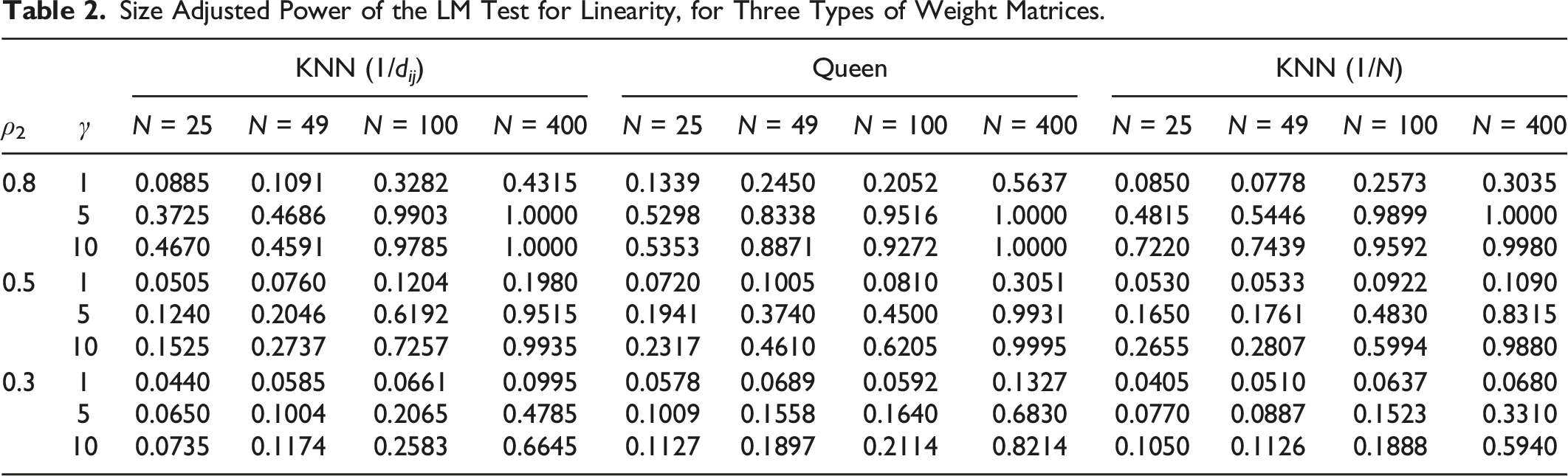
Size Adjusted Power of the LM Test for Linearity, for Three Types of Weight Matrices.
Boston House Prices
To demonstrate the practical application of the smooth spatial lag model, we utilize the Boston house price data from the open-source R package SpData. Our primary focus lies in estimating the spatial lag parameters, aiming to gain deeper insights into the influence of neighboring areas. Additionally, we intend to evaluate the model’s performance in capturing spatial dependencies and assess whether it outperforms a conventional linear spatial lag model.
Data
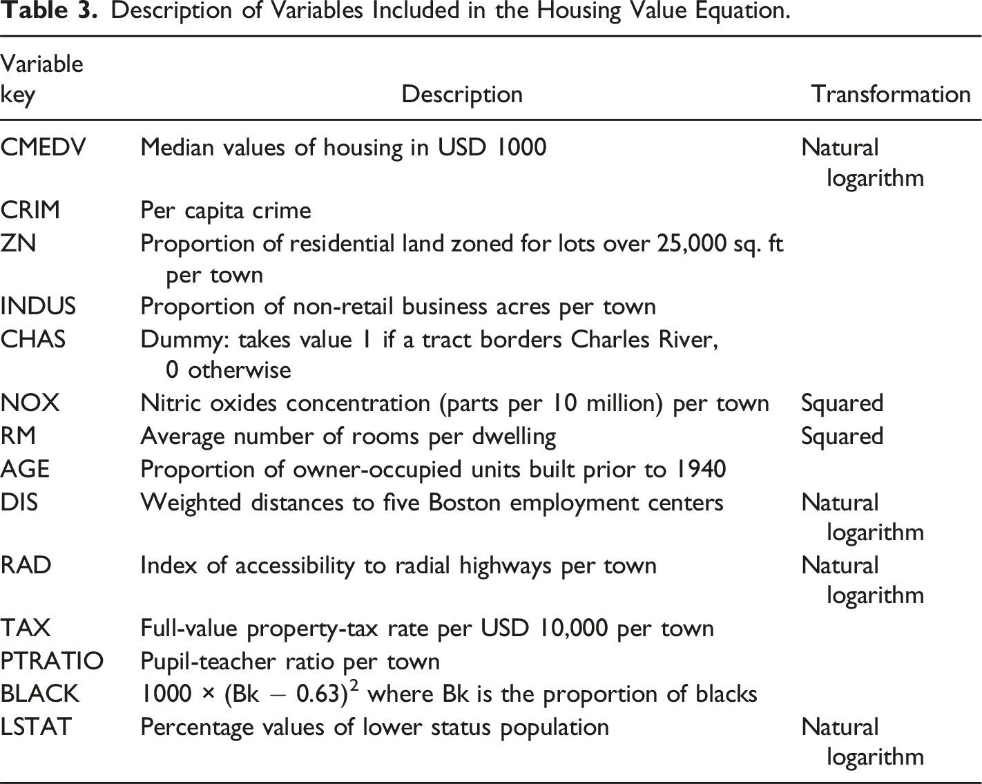
The data set consists of 506 census tracts within the Boston Standard Metropolitan Statistical Area (SMSA) in 1970. Initially analyzed by Harrison and Rubinfeld (1978) to study median house values and their relation to willingness to pay for clean air, the data has undergone minor corrections by Gilley and Pace (1996). In our application, we employ the same housing value equation as Harrison and Rubinfeld (1978) but introduce a spatial lag with smooth transitions. The dependent variable, denoted as y, represents the natural logarithm of median housing values in USD 1000 (ln(CMEDV)) and is depicted in Figure 2. The independent variables within X consist of two accessibility metrics, eight neighborhood variables, two structural attributes, and one air pollution variable, mirroring the variables used in Harrison and Rubinfeld (1978) (details provided in Table 3). Distribution of median house prices in the Boston area in 1970, measured in USD 1000. Natural breaks (Jenks) are used for classification. Description of Variables Included in the Housing Value Equation.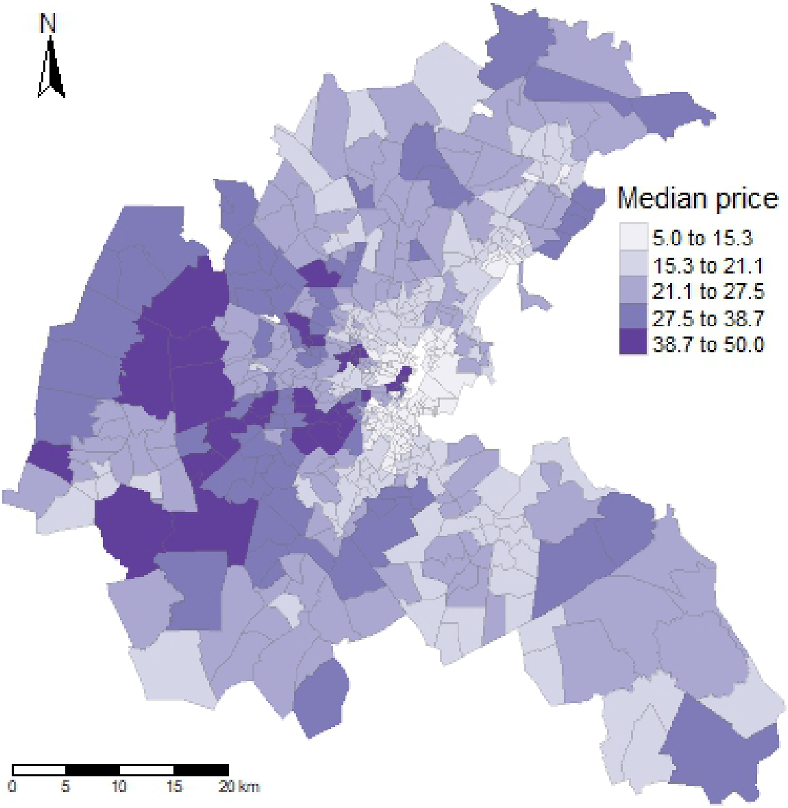
Testing
When estimating the smooth spatial lag model, the initial step involves defining the weight matrix W and identifying a suitable transition variable s. To ensure our findings are robust to different choices of weight matrices, we conduct the analysis using two different weight matrices. Firstly, we use a weight matrix based on k 2 nearest neighbors (KNN). Secondly, we use one based on the queen’s criterion.
Results of the LM Test for Linearity for all Potential Transition Variables.
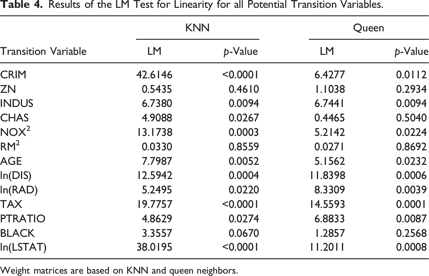
Weight matrices are based on KNN and queen neighbors.
Estimation
Estimation Results - KNN.
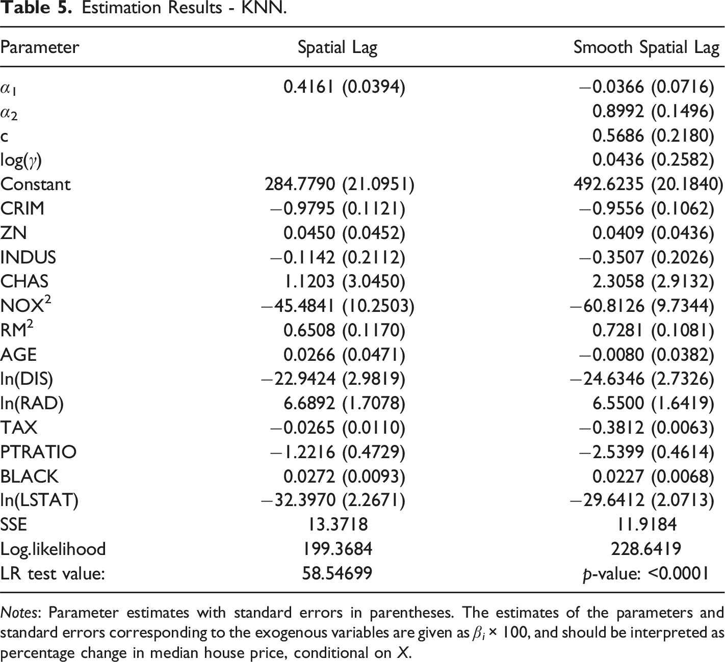
Notes: Parameter estimates with standard errors in parentheses. The estimates of the parameters and standard errors corresponding to the exogenous variables are given as β i × 100, and should be interpreted as percentage change in median house price, conditional on X.
Estimation Results - Queen.
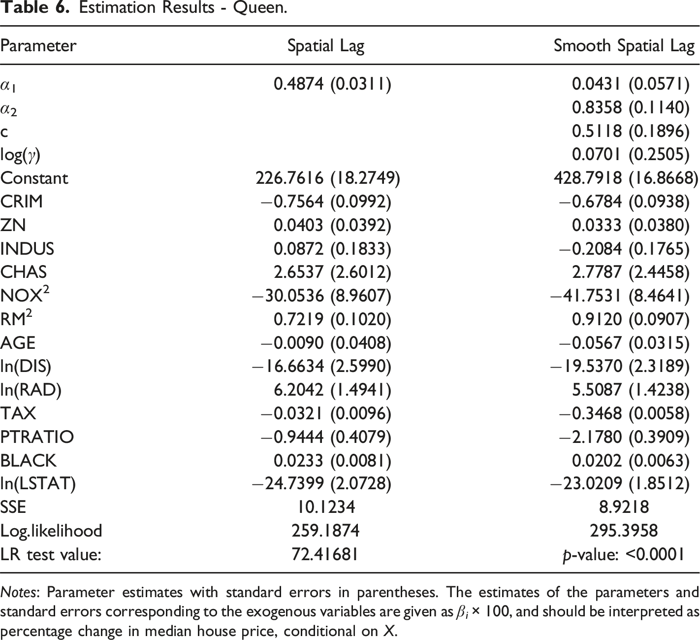
Notes: Parameter estimates with standard errors in parentheses. The estimates of the parameters and standard errors corresponding to the exogenous variables are given as β i × 100, and should be interpreted as percentage change in median house price, conditional on X.
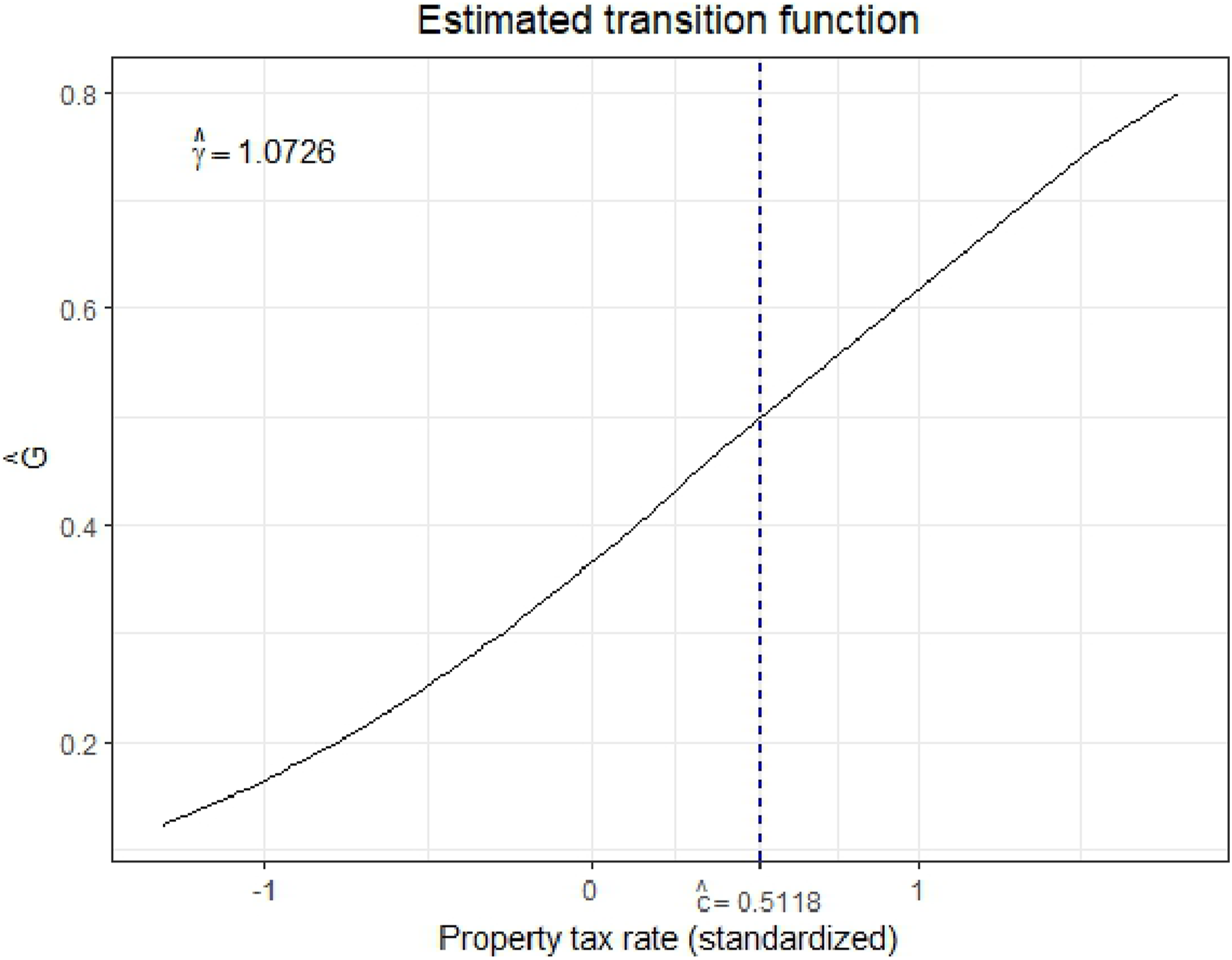
Estimated transition function G as a function of
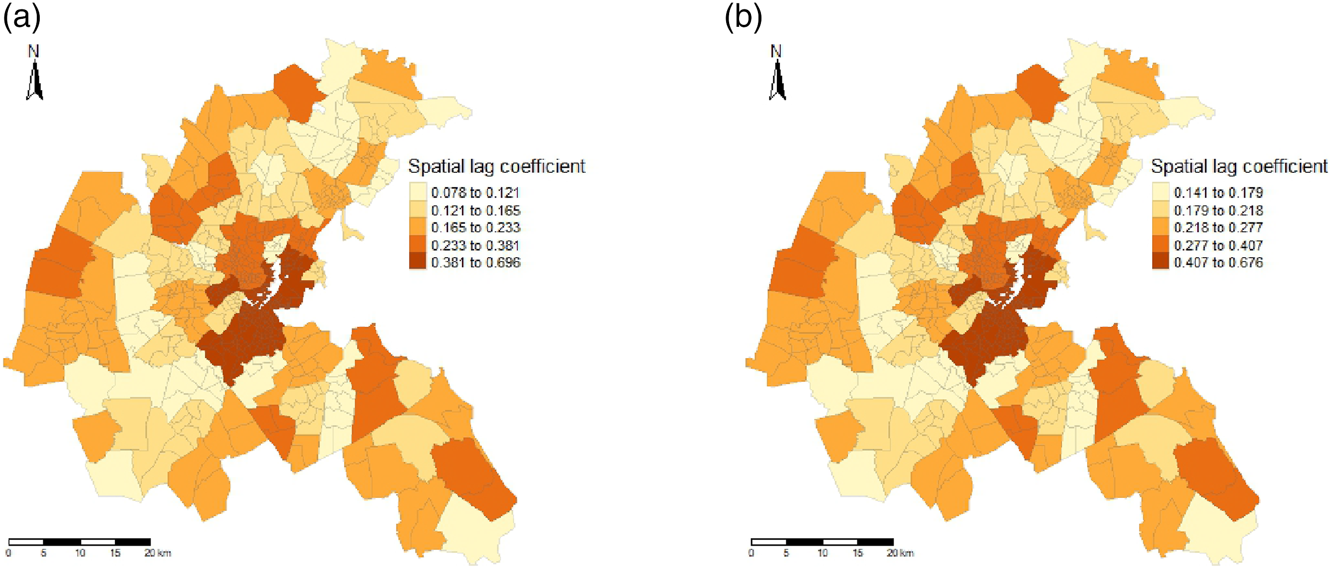
Estimated spatial lag parameters in different regions as determined by the transition function G. Natural breaks (Jenks) are used for classification. (a) KNN weights. (b) Queen weights.
Evaluation
Global Moran’s Test of Residuals.
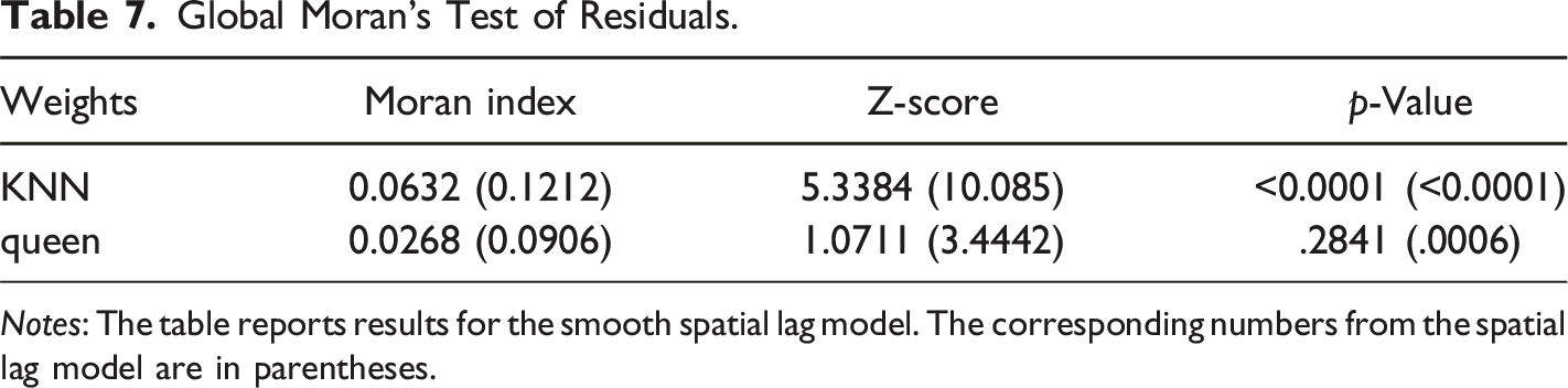
Notes: The table reports results for the smooth spatial lag model. The corresponding numbers from the spatial lag model are in parentheses.
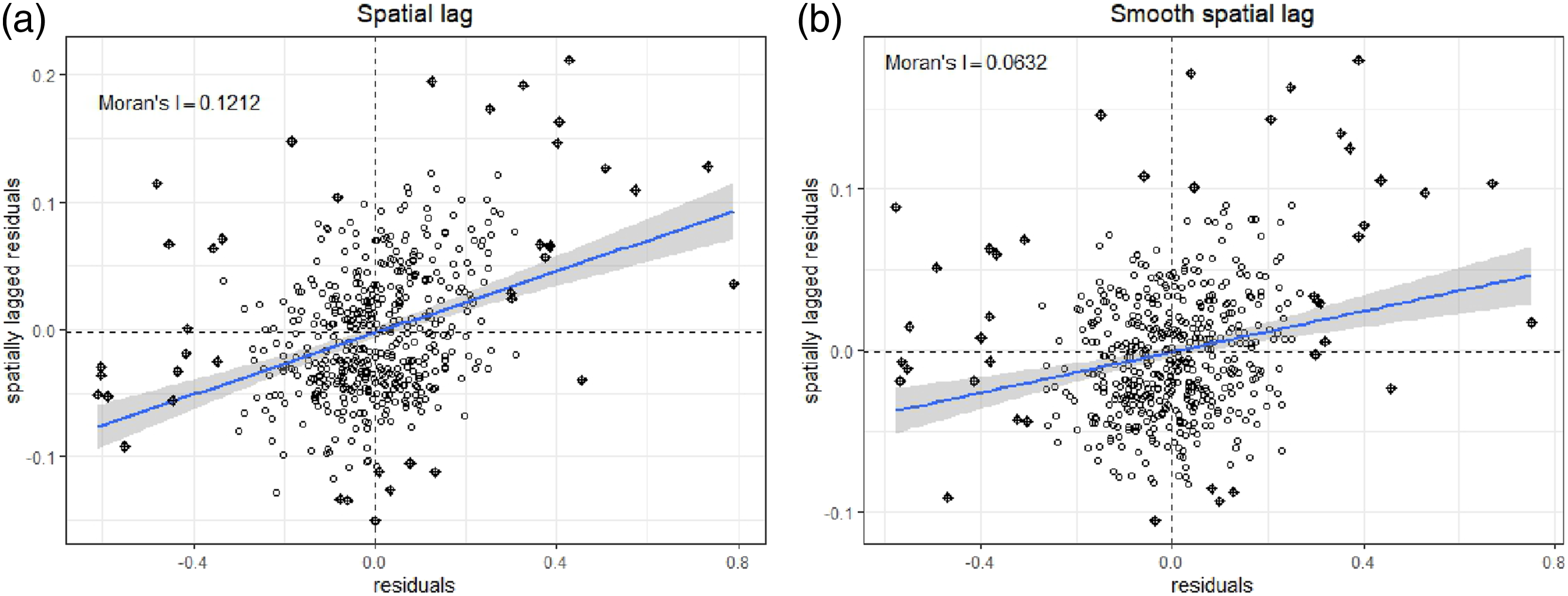
Moran scatterplot of residuals. Weights based on KNN. (a) Spatial lag. (b) Smooth spatial lag.
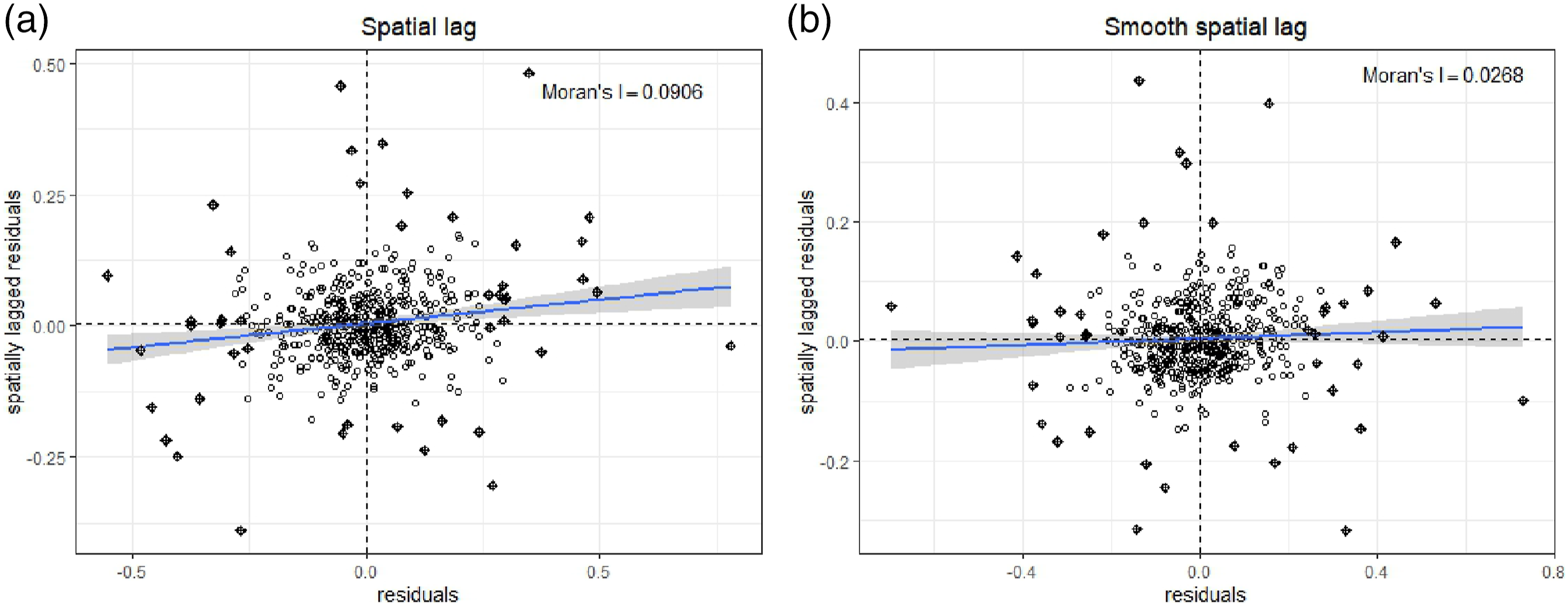
Moran scatterplot of residuals. Weights based on queen’s criterion. (a) Spatial lag. (b) Smooth spatial lag.
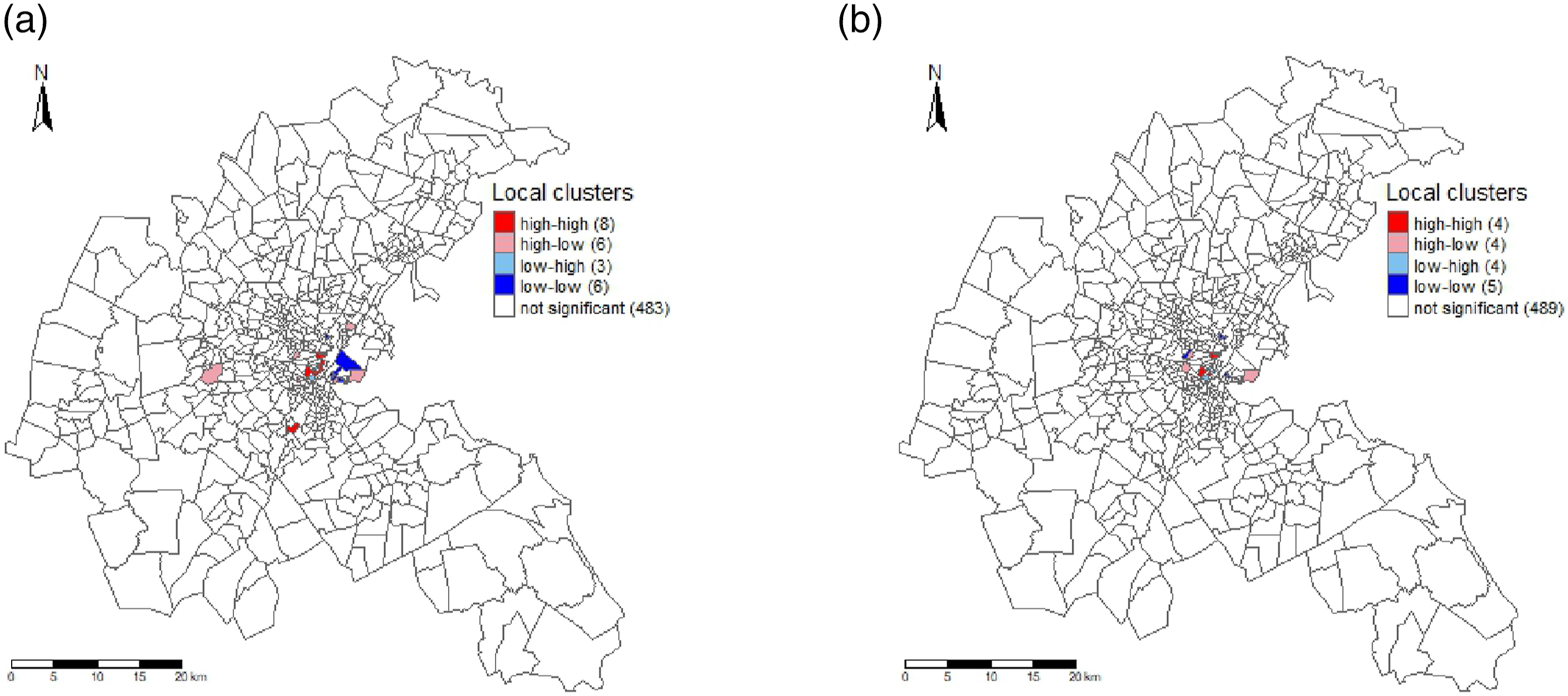
Additionally, we conduct a local cluster analysis using Local Indicators of Spatial Association (LISA) on the residuals, employing local Moran’s I as the LISA statistic. The results are visualized in the LISA cluster maps presented in Figure 7 (KNN weights) and Figure 8 (queen weights). These maps illustrate local clustering of model under- and over-predictions. “High-high” census tracts indicate spatial clustering of model under-predictions, while “low-low” indicates spatial clustering of over-predictions. “High-low” or “low-high” observations are considered spatial outliers. Comparing the residuals from the smooth spatial lag model with those from the spatial lag model, we observe an increase in areas with non-significant
3
clustering for both KNN weights (493 compared to 479) and queen weights (489 compared to 483). This signifies an enhancement in accounting for local spatial dependence for both types of weight matrices. Spatial clustering of residuals with weights based on KNN. “high-high” indicates clusters of model under-prediction, “low-low” denotes clusters of over-prediction, and “high-low” and “low-high” are spatial outliers. False discovery rates were used to adjust for multiple testing. (a) Spatial lag. (b) Smooth spatial lag. Spatial clustering of residuals with weights based on queen’s criterion. “high-high” indicates clusters of model under-prediction, “low-low” denotes clusters of over-prediction, and “high-low” and “low-high” are spatial outliers. False discovery rates were used to adjust for multiple testing.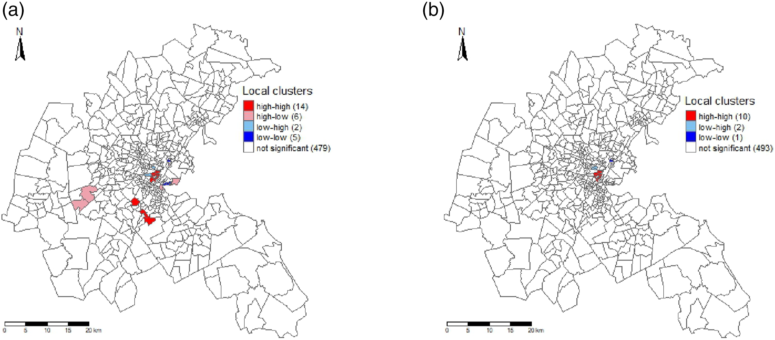
Conclusion
This paper introduces a novel approach to model spatial regimes for cross-sectional data. We propose using a spatial lag model wherein the spatial lag parameter smoothly varies between regimes. In the resultant smooth spatial lag model, we employ a logistic function as a transition function.
We discover favorable small sample properties for the developed test of nonlinearity across all three weight matrix specifications. The size-adjusted power of the test increases rapidly with the magnitude of the smoothing parameter, reflecting the degree of nonlinearity. While the test exhibits robust power for all weight matrices, it excels when the queen’s criterion is employed. When there is a distinguishable difference between the spatial effects of the two regimes, the power remains robust, even for moderate sample sizes. However, the good power properties do not extend to the cases where the difference between regimes is minimal and/or the sample size is small.
To exemplify the use of the model, an empirical application is carried out, estimating median house values in the Boston area. By subjecting all regressors in the model to the linearity test, the property tax rate is found to be an appropriate transition variable. The smooth spatial lag model is then compared to a linear spatial lag model. The linear model implies that the spill-over effect from neighbors is moderate and constant across all census tracts. On the other hand, the smooth spatial lag model suggests a large positive spill-over effect among census tracts that are above a certain threshold value in property tax. Conversely, a subtler dynamic for census tracts below the threshold can be observed. Here, the model implies that the spill-over effect is much smaller and can even oscillate between positive and negative values, depending on the weight matrix choice. Furthermore, the estimated shift between the two regimes is very smooth, meaning all observations fall somewhere between the extremes. This also implies that this model specification will be preferred over a threshold model with an abrupt shift. The smooth spatial lag further outperforms the linear spatial lag model regarding model fit and ability to account for spatial dependence. The analysis also implies that these results are robust for different choices of weight matrices.
Footnotes
Declaration of Conflicting Interests
The author(s) declared no potential conflicts of interest with respect to the research, authorship, and/or publication of this article.
Funding
The author(s) received no financial support for the research, authorship, and/or publication of this article.