What Teachers’ Unions Do for Teachers When Collective Bargaining is Prohibited

Abstract

Our research examines the relationship between teachers’ unions, teacher compensation, employment conditions, and turnover in Southern US states that prohibit the collective bargaining of public school teachers. We assess union strength by meet-and-confer status and the teacher union density of districts and estimate union impact using propensity score matching. We find that teachers’ unions are positively associated with teacher compensation and employment conditions, even in the absence of collective bargaining. Districts with strong unions have higher dismissals of nontenured teachers for poor performance and a lower attrition rate of qualified teachers, compared to districts with weak unions. This study shows that teachers’ unions in the United States still organize without formal labor-management institutions and make a significant impact on teachers’ work lives, even in a hostile legal environment toward unions.

Keywords

teachers’ unions collective bargaining meet-and-confer teacher compensation teacher dismissal teacher attrition I20 J51 J63

Most prior research on the effects of teachers’ unions in the United States has relied on analyses of data drawn from states where there is a collective bargaining (CB) agreement. However, even in states that ban CB, approximately half of public school teachers are unionized (Freeman and Han 2013), but we know very little about what teacher unions do in these states and what, if any, influence they exert over terms and conditions of employment. Our research focuses on states that prohibit CB. We make the first rigorous attempt to understand whether teachers’ unions in the US can affect teachers’ work lives without the institutions of CB and established methods of labor-management dispute resolution.

Some states that experienced teacher strikes in 2018–2019 include Arizona and North Carolina, in which CB of public school teachers is strictly prohibited and teacher strikes are illegal. Nevertheless, teachers in those two states did organize, make demands, and run strikes, and, in Arizona, conducted a successful strike that resulted in significant changes, such as pay raises, class size reduction, increases in support staff, and education spending. Based on these observations, we are interested whether, in the absence of CB, unions can make any significant impact on teachers’ work lives. More specifically, our research question is what teachers’ unions can do for teacher compensation and working conditions when they have extremely limited bargaining power in states that prohibit CB.

We set out to answer our research question using the School and Staffing Survey (SASS). We merge three waves of the SASS for the 2003–2004, 2007–2008, and 2011–2012 school years in our analysis of union influence on the terms and conditions of teachers’ employment in states that ban CB of public school teachers. We employ propensity score matching (PSM), using two metrics to assess the strength of teachers’ unions: meet-and-confer (MC) status and union density of public school teachers in each school district.

We find that teachers’ unions are associated with higher teacher compensation and better employment conditions, even when CB is not allowed. Teachers’ unions have a negative relationship with teachers’ attrition, although the effect size is not substantial. Teacher unionization is associated with a higher dismissal rate of underperforming teachers during the probationary periods.

This research makes several key contributions to literature. First, this study helps policymakers better understand how teachers’ unions are able to influence the educational system in legal environments where formal CB is unavailable. Second, we use district-teacher-matched data which allow us to identify employers of teachers and control for districts’ characteristics, including their financial status, which was unavailable in many studies. Third, we use both binary and continuous measures of teacher unionization to assess union strength in the absence of CB. Lastly, we offer a comprehensive analysis of teachers’ work lives and the teaching profession by examining the relationship between unions and teacher compensation (both salary and benefits), employment conditions in various aspects, as well as teacher turnover.

Literature

Studies on private-sector unions may not provide a guide to understanding how public-sector unions operate. Freeman and Medoff (1984) argue that improvement in employment conditions and increased labor productivity in firms in the private sector are the results of union voice through which employees can influence management. Their analysis also indicates that unions raise employee compensation through their “monopoly effect,” which primarily arises from their ability to impose costs on employers through CB and the right to strike. In this research, we examine whether unions can influence wages and working conditions without CB or the right to strike, in other words, without monopoly power, by focusing on unions of public sector employees and teachers in our public schools, in particular, from states where CB is not available.

Teachers’ Unions, Teacher Compensation, and Employment Conditions

Prior research suggests that teachers’ unions improve teacher earnings, but estimates vary considerably. Data, methods of analysis, periods of study, and institutional frameworks yield a wide range of union pay effects. There is considerable institutional variation across the United States. Some states permit and encourage teachers’ CB, but other states prohibit it. Some states permit teacher strikes, whereas other states outlaw them and impose severe penalties. Not only are there institutional differences in the US but there also are data limitations that hinder our ability to evaluate union effects on teachers’ earnings.

For example, are we measuring the union effect on earnings as wages/salaries or total compensation? Most often researchers settle for wages/salaries because of data limitations, even though we realize nonwage benefits, such as health insurance coverage, are expensive and a variable element in employee compensation. Many studies also cannot account for institutional variation: whether earnings are the product of local CB, state law, or alternative forms of union representation. Nor can they account for the range and scope of subjects in CB. We discuss the contradictory research below and address how our study improves on prior research.

The main source of data on the effects of teachers’ unions on wages has been the Current Population Survey (CPS), which does not directly ask about CB coverage to all respondents. The CPS asks whether an employee is a member of a “labor union or of an employee association similar to a union.” If the answer is “no,” only then is an employee asked whether he or she is “covered by a union or employee association contract?” It clearly overlooks the possibility that an employee is a member of a labor organization that does not engage in CB. This is mostly observed in the Southern states that do not permit public sector CB but in which many teachers still join unions. Other data sources often pose similar problems, especially when studies measure union strength with a simple CB status and yield a variety of conflicting results.

For instance, Frandsen (2016) reports, in his Current Population Survey Outgoing Rotation Groups (CPS ORG) panel data analysis, that CB laws have had a minimal effect on public school teachers’ hourly wages. On the other hand, Baugh and Stone (1982) find a union wage gap of about 12–22%, using the CPS ORG from 1974 to 1978, as union teachers made real wage gains while nonunion teachers incurred real wage declines in this highly inflationary period. Paglayan (2019), using a longitudinal dataset constructed from historical sources, finds that introducing teacher CB rights does not lead to higher education expenditures, and that the union wage premium may be capturing the teacher unionization that occurred in high-wage states, consistent with Frandsen's analysis. On the other hand, Hoxby (1996), using Census of Government data, reports a significant union premium. An analysis using data from the 1980s by Zwerling and Thomason (1995), using the 1984 Administrator Teacher Survey, finds a 5-percent union wage premium for teachers, which increased by 2.6 percent, with each 10-percent increase in teacher union density, not in CB.

The SASS asks a CB coverage question to districts in all US states, reducing measurement issues that appeared in the CPS, and several studies have relied on this information. Using the 1999–2000 SASS, Stoddard (2005) reports that unionization has a positive and large effect when a state switches from prohibiting CB in 1980 to the duty to bargain by 1990, regardless of the method for controlling for cost of living or amenities. Winters (2011), also using the 1999–2000 SASS, shows that CB and teacher union density increase salaries for experienced teachers by as much as 18–28%, but much less for beginning teachers.

West (2015), based on the 2003–2004 and 2007–2008 SASS, reports the differences between unionized and nonunionized districts, using both CB and MC measures. West finds that teachers in CB districts have higher starting salaries and larger step-and-lane increases. She also shows that higher salaries in MC districts are attributed to larger increases in salary schedules, but finds no evidence that MC districts have larger step increases than nonunion districts.

More recent research by Keefe (2018), using CPS ORG data 2013–2015, indicates that teachers’ union membership is associated with 5.1 percent higher wages and 5.4 percent higher total compensation for its members when compared with the compensation of public school teachers who are not union members. Hirsch, MacPherson and Winters (2011), using the CPS for 2000–2009 and the SASS for 1999–2000, estimate a union salary advantage for teachers of 5% arising from CB laws and coverage. In their recent meta-analysis of 19 studies with 77 estimates of union wage effects, Merkle and Phillips (2018) find that teachers’ unions produced an average wage impact estimated around 2–4.5% and observe that the union effects are confounded by the measures of union status, either at the individual or district level, and legal frameworks for labor-management relations. Marianno, Bruno and Strunk (2021) find that CB restrictiveness is positively associated with expenditure on students and educators.

Several studies find that unions significantly raise nonwage benefits and improve employment conditions. Freeman (1984; 1985) shows that employees who changed to unionized jobs received higher nonwage benefits, compared to those who stayed in nonunion jobs or moved out of union jobs. Freeman and Medoff (1984) attest unionized employees are 25–30 percentage points more likely to report having a pension plan than comparable nonunion workers. Delaney (1985) finds that unionized districts in Illinois had a larger “fringe benefit index” compared to districts without bargaining contracts. Based on Ohio school district data, Cook, Lavertu and Miller (2021) show that CB increases teacher benefits, as well as salaries. Hirsch, Macpherson and DuMond (1997) demonstrate that because unions provide workers with information concerning their rights and legal benefits, as well as education in filing claims, union workers are more likely to file workers’ compensation claims and to receive compensation benefits than similar nonunion workers. Podgursky (2003) argues that Chicago teachers’ unions effectively increase pension contributions for their members in public schools. Hoxby (1996) shows that teacher unionization decreases the student–teacher ratio by 1.7 students per teacher. Han (2019) finds that teachers’ unions reduce the number of contract days and required hours for base salaries.

Teachers’ CB was initially aimed at improving pay and working conditions but eventually expanded to improving professional status and increasing autonomy (Cole 1969). Nevertheless, Rosenberg and Silva (2012) show that more than 70 percent of teachers report that rank-and-file teachers usually have very little control over what goes on in their schools. Studies on union certification elections reveal that employees who feel they lack control over work are more likely to unionize (Barling, Fullagar and Kelloway 1992). Healthier professionalism and greater control in their classrooms may also influence teachers’ confidence and career satisfaction. Indeed, Han and Keefe (2021) find that the morale of union teachers is higher than that of nonunion teachers in the states that have duty-to-bargain laws and allow agency fees.

Dispute resolution frameworks under CB also appear to affect teacher outcomes. A 43-state analysis of the impact of dispute resolution mechanisms on the wages and hours of public school teachers by Zigarelli (1996) found evidence that the right to strike increased teacher wages by 11.5%; arbitration availability was associated with a wage effect of 3.6%; and fact-finding had no significant influence on earnings. A direct comparison of the right to strike and the right to arbitrate indicated that a legal right to strike affords teachers greater power to increase their earnings.

Although some studies indicate that teachers’ unions and their CB increase teacher earnings and expenditure, other studies also suggest that teachers’ unions do not affect public expenditure on education. For instance, using data on teachers’ union certifications from Iowa, Indiana, and Minnesota, Lovenheim (2009) shows no net impact of teachers’ unions on per-student district expenditures. Lindy (2011), using the 1999 sunset and 2003 reauthorization of CB rights of public employees in New Mexico, finds that mandatory bargaining has no significant impact on per-pupil expenditures. Fransden (2016) shows that, when using the state fixed effect models, the effects of CB laws are very close to zero for all specifications of per-pupil salary and per-pupil expenditure. This finding follows the state pattern on wages, where states with higher expenditures on education and higher salaries were also the states that adopted CB for their public employees. CB may not cause higher education expenditures, but it is associated with greater expenditures overall.

Teachers’ Unions and Turnover

Since teachers’ unions raise wages and improve employment conditions, we should expect that unionization would reduce employee voluntary job turnover (Hom and Griffeth 1995; Imazeki 2005; Murnane and Olson 1990). Researchers find that unions enhance members’ well-being by improving working conditions, potentially deterring workers from leaving their jobs (Eberts and Stone 1987; Goodlad 1984; Ingersoll 2001; Mueller and Price 1990; Rosenholtz 1989; Steer and Mowday 1981). Freeman (1980) presents that unionism reduces quits and raises the job tenure of employees by providing a “voice” alternative, a channel to express their concerns in the work place when dissatisfied with employment conditions. Through this “voice” channel, unions also serve workers by articulating worker preferences, improving communication between employers and employees, and enhancing employee's commitment to the organization (Addison and Belfield 2004; Batt, Colvin and Keefe 2002; Gunderson 2015). Similarly, Rees (1991) shows that teachers with strong grievance procedures in their contracts had a lower probability of quitting than those working under weaker grievance procedures. Han (2020) finds that teachers’ unions reduce the voluntary quits of novice teachers with higher qualifications, assessed by Highly Qualified Teachers (HQT) certification.¹

Teachers’ unions may make it easier for schools to recruit and retain qualified teachers, enabling them to set higher standards for retention and tenure, leading to greater dismissals. The literature on teacher dismissals is often unable to distinguish between voluntary and involuntary resignations. Consequently, only a few studies have looked at the direct effect of teachers’ unions on teacher dismissal in public schools. Bridges (1986) and Theobald (1990), for instance, each report teacher dismissals in public schools in a single state, where it is unclear whether a dismissal decision is based on teacher performance or on certain shocks in the local labor market, such as school closings or layoffs. West (2015) reports that unionization is positively correlated with the number of junior teachers dismissed for poor performance but not strongly correlated with the number of senior teachers’ dismissals.

Han (2020) also finds that districts with bargaining contracts have higher dismissal rates for underperforming nontenured teachers, arguing that the higher pay unions negotiate for their workers provides economic incentives to districts to be more selective before granting tenure to teachers. She shows that CB has no significant impact on the dismissal rates of tenured teachers, rejecting the common claim that unions overprotect bad teachers.

Teachers’ Unions Without CB Rights

Most prior studies regarding union effects on teachers’ employment conditions and teacher turnover examine unions’ roles where CB is available and widely used. In states that prohibit CB, however, teachers’ unions have no legal right to any of these dispute resolution procedures, possibly leading to lower pay and poor employment conditions. Nonetheless, Han (2019) finds that half of teachers still join unions in states that do not allow teachers’ CB and argues that a CB contract is not a necessary condition for teachers’ unions to operate.

What are the potential ways in which unions could shape working conditions and wages in the absence of CB? First, the “voice” role of unions may still be important during nonbinding MC agreements. In addition, unions use their political power to act as lobbyists for a variety of policies in an attempt to gain other advantages beyond CB contracts. Thus, the ability to gain political support through membership voting is crucial (Demsetz 1993; Rosenfeld 2010).

A body of research also establishes the role that teachers’ unions play as an interest group in shaping state policy (Finger 2018a; Hartney and Flavin 2011; Marianno 2019; Moe 2011). Finger (2018b) shows that unions with higher memberships were deemed more effective in securing their policy objectives. Brunner, Hyman and Ju (2020) find that districts with strong teachers’ unions increase spending with state aid and spend the funds primarily on teacher compensation, whereas districts with weak unions use state aid primarily for property tax relief. The authors also show that greater expenditure increases in strong union districts lead to larger increases in student achievement.

Therefore, it is essential to understand what unions can do for their members and the teaching profession in general in the most hostile legal environment. Our study aims to fill this knowledge gap and shed new light on unions’ role in public education in the absence of CB that has been largely ignored in literature.

Our study focuses on districts from states that share a similar legal environment toward teachers’ unions. As of 2012, eight states (Alabama, Arizona, Georgia, Mississippi, North Carolina, South Carolina, Texas, and Virginia) did not have CB laws for public school teachers. Thus, a binary measure for the existence of bargaining contracts between districts and unions, or a simple categorization of state legislation (whether or not a state allows CB of public sector workers), cannot measure the true variation of teacher unionization in these states.

Two recent studies provide empirical background for our study. Exploiting nationally representative data, Han (2019) shows that teachers in states that ban CB of teachers are still able to receive a higher base salary through MC and higher union membership, although the magnitude of union effects is much smaller than in pro-union states that mandate CB and allow the collection of agency fees. Relying on data that cover all US districts, Han and Keefe (2020) find that teacher unionization is positively associated with students’ academic performance, even in the states that prohibit CB of teachers. In particular, they find that MC has associated with significant and substantial improvements in students’ NAEP scores for both math and English.

Building on these studies, it is our goal to add to literature by examining how teachers’ unions, even without the institutional framework that normally accompanies CB rights, influence teachers’ work lives and by exploring potential channels through which unions are able to affect public education. Our study is the first to investigate the influence of teachers’ unions on both voluntary and involuntary teacher turnover, as well as teachers’ pay and working conditions in states that prohibit CB.

Data

The primary data source of this study is the SASS, nationally representative data. We construct a district-teacher matched dataset by linking data on teachers and districts within each wave of three survey years (2003–2004, 2007–2008, and 2011–2012 school years) of the SASS. One year after the SASS is collected, teachers who left the teaching sector are surveyed, constituting the Teacher Follow-up Survey (TFS) for former teachers. We combine the district-teacher-matched SASS with the TFS to construct the SASS-TFS dataset for each survey year and merge them to form a pooled cross-sectional dataset covering the 2003–2013 school years. We also combine three waves of the SASS data to construct pooled 2003–2013 district-level data.

The advantage of the SASS data is that it provides integrated data on teachers’ employment conditions, their demographics, attitudes toward teaching, and school and district characteristics. Its main shortcoming is that the samples are slightly dated, but what we seek to predict are teachers’ relative conditions, which are largely slow changing.²

This study also utilizes the School Districts Finance Survey (SDFS), which details annual fiscal data for every US school district. Two of our control variables, districts’ total revenue and property tax rate (property tax/local tax revenue), come from the SDFS. Thus, controlling for districts’ financial status and educational inputs, we are able to investigate if districts with stronger unions allocate more resources toward teachers.

Additionally, we merge information from the Comparable Wage Index (CWI), which measures the salaries of occupations that are comparable to teaching in the local labor market (Taylor and Fowler 2006). This enables us to control for locality differences, such as the cost of living in each district.

We limit our samples to eight states (Alabama, Arizona, Georgia, Mississippi, North Carolina, South Carolina, Texas, and Virginia) that did not have explicit CB laws for public school teachers during our study period.

Our measures of teacher unionization come from the SASS. We use two measures of teacher unionization to assess union strength in the absence of CB. One is teacher union density in each district, which we compute from the union membership status of individual teachers within the district. We infer that a higher percentage of union membership in a district will translate into greater influence in terms and conditions of employment. The second measure is whether the district has either a formal or informal MC process with the union. During MC, unions and management exchange views and discuss proposals that can lead to an agreement likely to affect the outcomes, but, unlike CB, an MC agreement is legally unenforceable.³

Using the 2004, 2008, and 2012 Current Population Survey Merged Outgoing Rotation Groups (CPS MORG), we construct a proxy variable for private sector union density in a district, which we use as an additional control variable. Based on the zip codes of the schools and whether those schools are in either a metropolitan statistical area (MSA) or a non-MSA, we compute the average union membership rate of private sector workers that can be assigned to each school district. The average private sector union density in districts provides information on the general atmosphere of the political environment toward labor unions and industrial/occupational base of the local economy.

For a comprehensive analysis, we look at various outcomes of teachers: teacher compensation, employment conditions, attrition, and dismissal. We have multiple measures for teacher compensation. We first use districts’ salary schedules that are based on teachers’ education attainment and experience. We have four categories or “lanes” of salary schedules: salary for teachers with bachelor's degree with zero experience, bachelor's degree with 10 years of experience, master's degree with zero experience, and master's degree with 10 years of experience. Based on these salary schedules, we construct two new variables for returns to 10 years of experience: Returns to experience for BA and Returns to experience for MA. Returns to experience for BA is computed by (base salary with 10 years of experience – base salary with no experience)/base salary with no experience for teachers with bachelor's degree. Returns to experience for MA is computed by (base salary with 10 years of experience – base salary with no experience)/base salary with no experience for teachers with master's degree. Additionally, we use districts’ average benefit per teacher, computed by total benefit expenditure divided by number of teachers, and average total compensation per teacher (sum of average salary per teacher and average benefit per teacher) as additional measures for teacher compensation. For all these variables, we use log-transformation to deal with skewedness in data and to make patterns in the data more interpretable.

By working conditions, we refer to the school environment and terms and conditions of teachers’ employment. We assess teachers’ working conditions with various metrics: Class size (pupil per teacher) and number of school days per year are used to measure overall work hours, a binary indicator for districts that reward teachers who have attained National Board for Professional Teaching Standards (NBPTS) certification to capture teachers’ professional development, a control factor to quantify teacher autonomy, and a morale factor to gauge teacher satisfaction and enthusiasm in their profession.

In addition, we assess teacher attitudes in their workplaces in two categories: teacher control factor to quantify teacher autonomy in their classroom and teacher morale factor to gauge how enthusiastic and satisfied teachers are in their profession. Each category is comprised of various teacher survey questionnaires, whose answers are scaled between 1 and 4 of the SASS, from all three waves. For instance, one question under the teacher control category questionnaire asks: “How much actual control do you have in your classroom at this school in selecting textbooks and other instructional materials?” The teacher morale category includes questions such as: “To what extent do you agree or disagree with the following statement: the stress and disappointments involved in teaching at this school aren’t really worth it?” We coded the answers to each question such that a higher number represents higher control and higher morale (see Appendix I for all the questionnaires included in each category). We employ a principal component analysis to aggregate these questions into two manageable categories. This factor analytical approach produces a single factor for teacher control and teacher morale.⁴

Teacher attrition is measured with the binary indicator such that Quit = 1 if teachers who were in the classroom during the 2011–2012 (2007–2008) school year voluntarily left teaching in the 2012–2013 (2008–2009) school year for reasons other than retirement, and Quit = 0 if the teachers remained teaching in 2012–2013 (2008–2009).⁵

We measure teacher dismissal rate by number of teachers dismissed due to poor performance divided by number of newly hired teachers in each district. For clarity on dismissal incidence, we separate nontenured teachers’ dismissal from tenured teachers’ dismissal.

Appendix II provides details on data sources and variable description, and Appendix III provides summary statistics of key variables from the pooled cross-sectional SAS-TFS dataset covering the 2003–2004, 2007–2008, and 2011–2012 school years. The average union membership rate is fairly high, approximately 50%, even in the states that ban CB of public school teachers, and formal and informal MC coverage for these states is about 15%. Most districts in states with no CB rights have no agreement (NA) with unions. Teacher salary schedules rise with the teacher's education attainment and experience. Returns to 10 years of experience are about a 20 percent increase in salary. The average benefit per teacher is about $21,700, and the average total compensation per teacher is about $62,300 between 2003 and 2013. Class size is about 16 pupils per teacher, and, on average, 45 percent of districts reward teachers for attaining NBPTS. The number of school days is about 180 days per year. Approximately 2.3 percent of teachers voluntarily quit for other than retirement reasons, either between the 2007–2008 and 2008–2009 school years or between the 2011–2012 and 2012–2013 school years. Overall, each district dismisses about 5.7 nontenured teachers and 3.7 tenured teachers for poor performance per year.

Figures 1 through 3 describe the relationship between teacher unionization and teacher outcomes by comparing the mean values by MC status. Figure 1 presents that teacher salary schedules, average benefits, and average total compensation are higher in MC districts than in NA districts. For instance, on average, the salary schedules for teachers with master's degrees are $1,560 higher in MC districts than in NA districts. The average total compensation is $2,220 greater for teachers in MC districts. All these mean differences between MC and NA districts are statistically significant. In Figure 2, employment conditions, measured by various metrics, are more favorable in the MC districts than in the NA districts. MC districts tend to have smaller class sizes and are more likely to reward teachers for obtaining NBPTS. Teachers in the MC districts report higher morale and greater control than teachers covered by no such agreement. Figure 3 shows that, on average, MC districts have a lower teacher attrition rate than the NA districts, and poor-performing teachers are less likely to be dismissed in the MC districts than in the NA districts. However, none of these differences in teacher turnover by MC status is statistically significantly different from zero.

Figure 1.

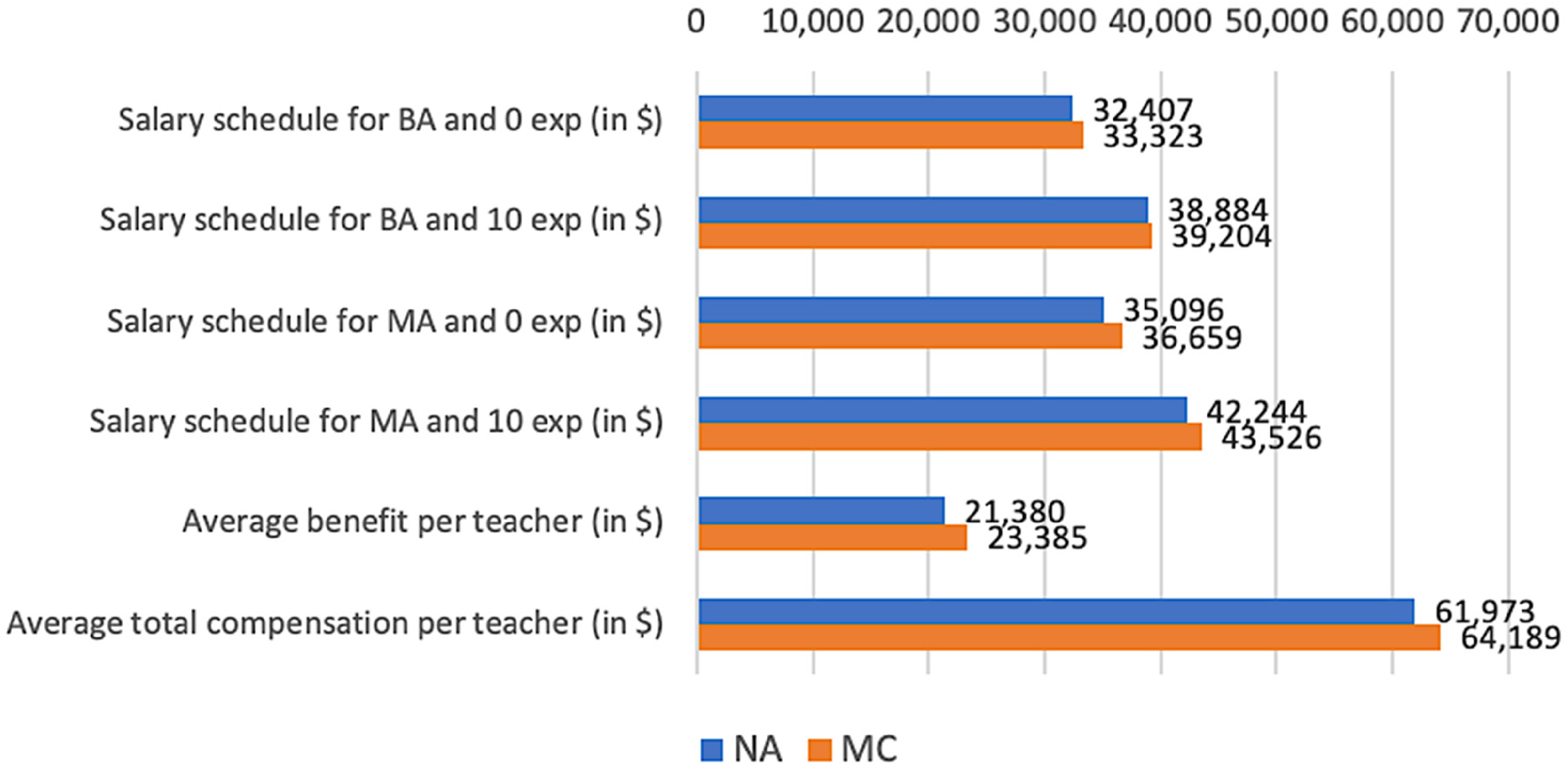
Teacher compensation by meet-and-confer status.

Figure 2.

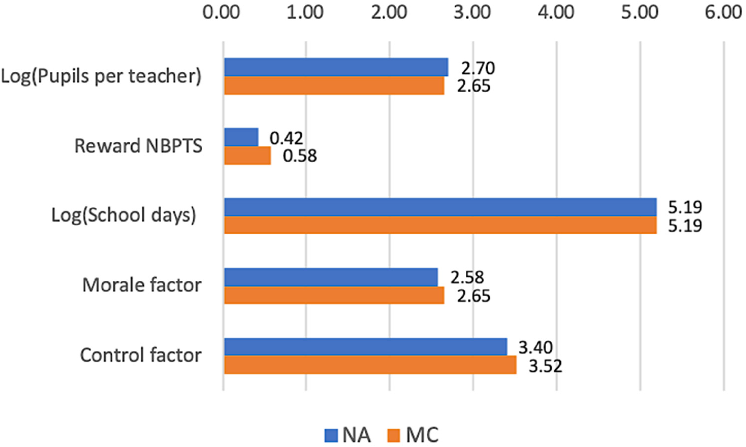
Teacher working conditions by meet-and-confer status.

Figure 3.

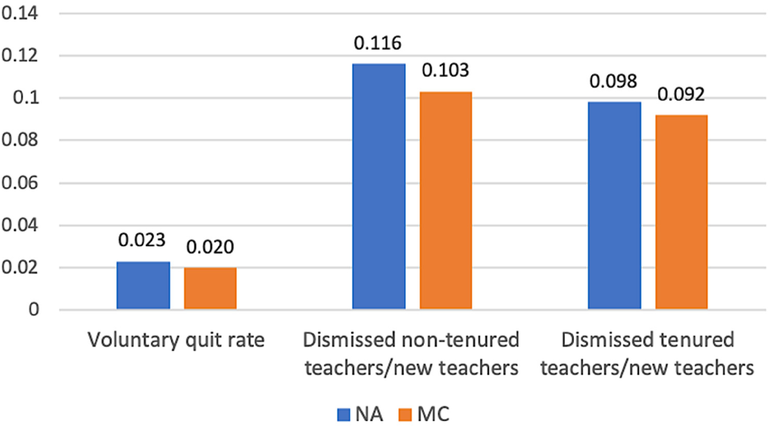
Teacher turnover by meet-and-confer status.

The pattern shown in Figures 1 through 3 may be affected by other characteristics of districts and teachers that are correlated with the presence of teachers’ unions. This indeed seems likely, as the mean characteristics of districts and teachers do differ by MC status, according to summary statistics reported in Table 1. Panel A of Table 1 compares districts’ characteristics and panel B compares teachers’ characteristics. Districts covered by an MC agreement have higher union density for public school teachers and higher union density for private sector workers. MC districts tend to have more Hispanic but fewer black students, larger student enrollment, a lower fraction of students enrolled in free/reduced-price lunch programs, greater district revenue, and be located in an urban area than is the case in NA districts. MC districts are also more likely than NA districts to reward teachers with NBPTS certification and to have longer probationary periods before granting tenure to teachers. Teachers in MC districts are more likely to be male and Hispanic than those in NA districts. Compared to teachers in NA districts, MC teachers appear to have stronger qualifications, assessed by the percent of teachers with master's degrees, regular certification, and certified HQT.

Table 1.

District and Teacher Characteristics by Meet-and-Confer Status.

	MC districts	Non-MC districts	Difference (SE)
Panel A: School District Characteristics
Union density of public school teachers	0.610	0.470	0.14***(0.019)
Union density of private sector workers	0.027	0.017	0.01***(0.001)
Fraction of Hispanic students	0.224	0.18	0.044***(0.014)
Fraction of Black students	0.204	0.262	−0.058***(0.015)
Fraction of Asian students	0.018	0.014	0.004***(0.001)
Fraction of Other students	0.058	0.023	0.035***(0.007)
Fraction of Hispanic teachers	0.082	0.07	0.012 (0.010)
Fraction of Black teachers	0.119	0.151	−0.032**(0.015)
Fraction of Asian teachers	0.009	0.006	0.003***(0.001)
Fraction of Other teachers	0.017	0.008	0.009***(0.003)
K-12 enrollment (in thousand)	14.58	8.8	5.78***(0.99)
All teachers	985.1	652.3	332.8***(71)
New teachers	110.5	68.2	42.3***(8.03)
% Free/reduced-price lunch programs	53.1	57.1	−4.0***(1.3)
CWI	1.11	1.1	0.010 (0.007)
Total district revenue (in million $)	148.3	88.2	60.1***(10.75)
% Urban	28.9	17.3	11.6***(2.2)
% Reward teachers with NBPTS certification	58.2	42.2	0.16***(0.028)
Length of probationary period	3.03	2.73	0.30***(0.048)
Observations	330	1,800
Panel B: Teachers Characteristics
Male	0.305	0.285	0.020**(0.008)
Full time	0.942	0.946	−0.004 (0.004)
Experience	12.90	12.83	0.070 (0.189)
Hispanic	0.073	0.060	0.013***(0.004)
Black	0.119	0.153	−0.034***(0.006)
Asian	0.015	0.013	0.002 (0.002)
Other	0.036	0.022	0.014***(0.003)
Master's degree	0.438	0.352	0.086***(0.009)
Education specialist	0.062	0.064	−0.002 (0.004)
Doctorate or professional degree	0.009	0.014	−0.005**(0.002)
Secondary school	0.710	0.723	−0.013 (0.008)
Special education	0.122	0.114	0.008 (0.006)
Charter school	0.003	0.062	−0.059***(0.004)
Regular certification	0.91	0.89	0.020***(0.006)
Highly Qualified Teacher (HQT)	0.887	0.838	0.049***(0.008)
Observations	2,780	14,640

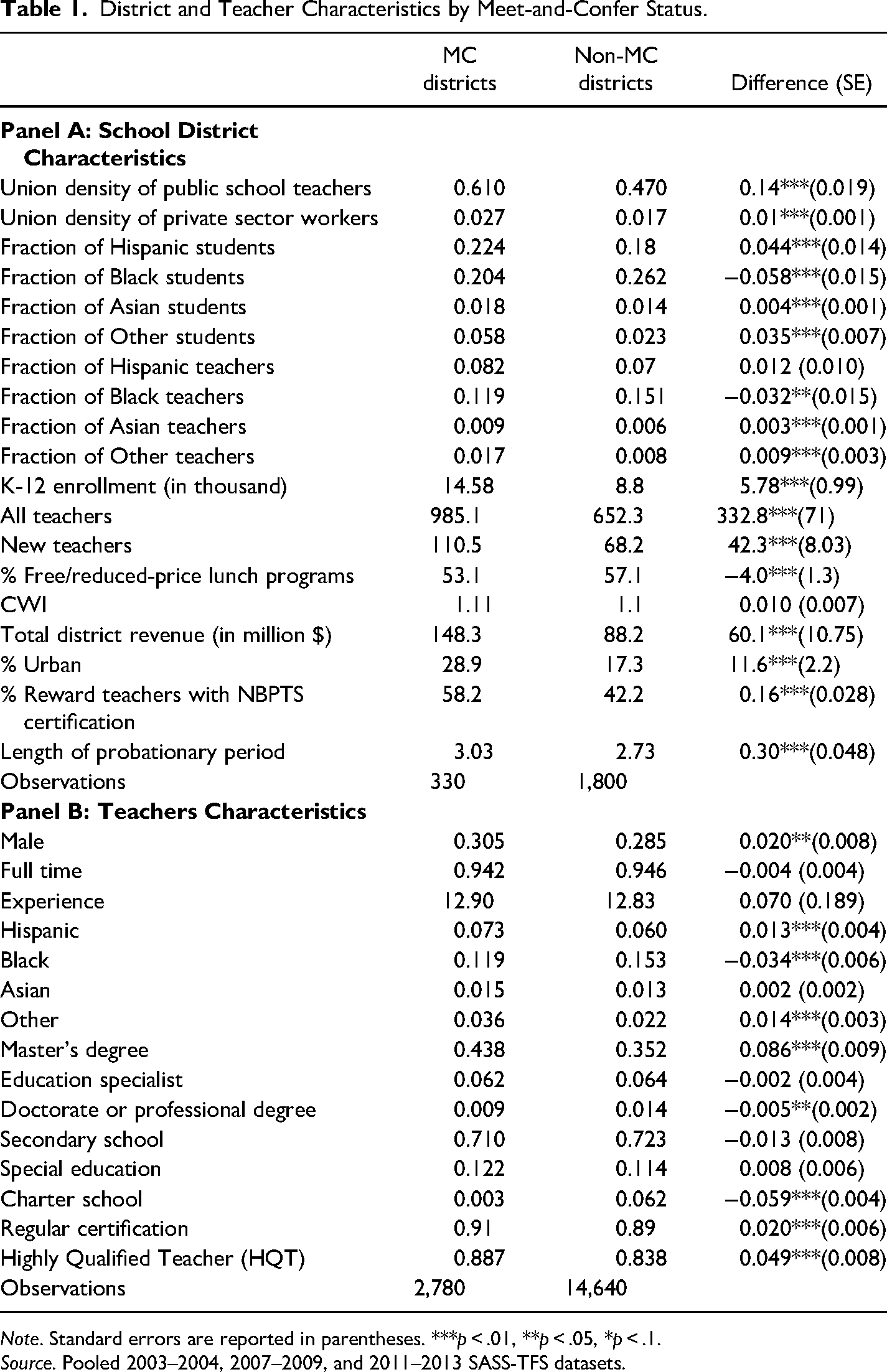
Note. Standard errors are reported in parentheses. ***p < .01, **p < .05, *p < .1.

Source. Pooled 2003–2004, 2007–2009, and 2011–2013 SASS-TFS datasets.

Methods

To control these characteristics of districts and teachers that are presented in Table 1, we can employ ordinary least squares (OLS) analyses of the correlation between teacher outcomes and unionization. The OLS estimators, however, will suffer from omitted variable bias if certain characteristics of districts are associated with both unionism and the outcome of interests.

One such factor is political inclination, such as the general attitude toward public spending and the tax system. For instance, if the districts that have been favoring the Democratic party for the past several decades tend to adopt public policies that allocate more resources to public education, the OLS regressions will overestimate the union effects. If, on the other hand, districts with less educational resources are more likely to produce a pro-union atmosphere, partly because more teachers would want to unionize for greater bargaining power and support in those districts, the OLS estimates will be biased downward.

In addition, teachers in larger districts are able to unionize more efficiently, due to the lower cost of organizing (more members covered by a single union representative), and unions in larger districts may have greater bargaining power (Brunner and Squires 2013; Rose and Sonstelie 2010). Thus, district size can potentially allow more resources for teachers, leading to the overestimation of union influence in large districts. The industrial/occupational base of the local economy, such as urbanism of districts, may also play an important role because metropolitan districts tend to offer a greater variety of career options outside of teaching, compelling districts to pay their teachers more competitively while raising teacher attrition.

To address these endogeneity issues, we first rely on other sources of data to control for various community characteristics, including property tax (in percent of local revenue), union membership rate of private sector workers, cost of living (measured by CWI), and the urbanism of each district. These are included, in addition to basic district-level control variables such as race and ethnicity composition of students and of teachers in percent, K-12 student enrollment size, number of teachers, and fraction of students eligible for free or reduced-price lunch programs. For teacher-level analysis, we add teacher's gender, race/ethnicity, experience, full-time status, education level, a dummy for secondary school, special education, and charter school teacher, and certification status as additional control variables.

Even though we control for various factors to minimize potential omitted variable bias, it does not address potential selection bias that can still pose an endogeneity problem. For instance, in the states prohibiting CB, MC is always an available option, but some districts have MC while others do not, and this selection issue may distort the causal inference of the analysis. We attempt to address this issue by employing PSM.

Considering MC as a treatment, we define districts with MC as treated units and NA districts as nontreated units. We construct a model of the propensity of having MC and match each MC district to an NA district with a probability (propensity) of having MC similar to that of the MC districts. Assuming the treatment decision is random conditional on observable pretreatment characteristics X (i.e., “selection on observables”), we specify the propensity score (p) of receiving treatment as a function of X that determines the selection into treatment such that: $p_{kt} = P r (D_{kt} = 1 | X_{kt} = x)$ , where D represents whether the district receives the treatment (MC). To estimate the propensity score, p(X), we use the following logit regression:

M C_{kt} = b_{0} + b_{1} X_{kt} + ε_{kt},

(1)

where MC equals to 1 if an MC agreement exists between a district and the union representative and 0 if no such agreement exists. X represents the district-level covariates that determine selection into treatment.⁶ The p(X) is the predicted value of MC we estimate from equation (1).

We use nearest neighbor (NN) matching with one neighbor based on the propensity score p for a matching algorithm. NN matching takes each treated unit and searches for the control unit with the closest p, so all treated units find a suitable match. We apply the “with replacement” option to avoid bad matches and to reduce the potential bias so that a control unit can be the best match for more than one treated unit.⁷ In addition, we impose the common support restriction to improve the quality of the matches, so only the observations whose p belongs to the intersection of the regions of the p of the treated and control units are considered in our analysis. To be consistent with Abadie and Imbens (2008), we rely on robust standard errors, instead of bootstrapping standard errors, when computing standard errors for our NN matching estimator.

Once each treated unit is matched with a control unit based on the p, we compute the mean difference of outcome variables between the treated and control units. Then, we obtain average treatment effect by taking the weighted average of these mean differences. Ideally, this matching process allows us to attribute the entire difference in the outcome variables between the treated and nontreated units as resulting from districts’ MC treatment.

To demonstrate the success of the matching and to test the balancing property, we perform several tests. First, we compute the percent of bias for each covariate that is used to estimate the propensity score.⁸ After the matching, the percent of bias for most covariates for the MC treatment is less than 5%, as recommended, suggesting that our covariates are well-balanced and that matching reduced the likelihood of biased treatment. Appendix IV summarizes the mean comparison of selected covariates and the percent of bias after matching, based on MC status.

We also check pseudo-R² values from the logistic regression model for treatment in the unmatched raw data (before the matching) and then again in the matched data (after the matching). All the pseudo-R² statistics calculated from our PSM range between 0.21 and 0.27 before the matching but very close to 0 after the matching. The pseudo-R² indicates how well the regressor X explains the treatment probability. Thus, there should be no systematic differences in the distribution of covariates between both treatment and control groups after matching. This implies that the baseline factors must be no longer predictive for determining the treatment group, and our small pseudo-R² after the matching demonstrates that adequate balancing was achieved.

In addition, we check the distribution of propensity scores in Figure 4(a) to examine the range of common support and visually inspect the matching. The histogram displays that the treated and untreated groups have symmetrical distributions of propensity scores, implying that matching has constructed good control units for the treated units on the observables.

Figure 4.

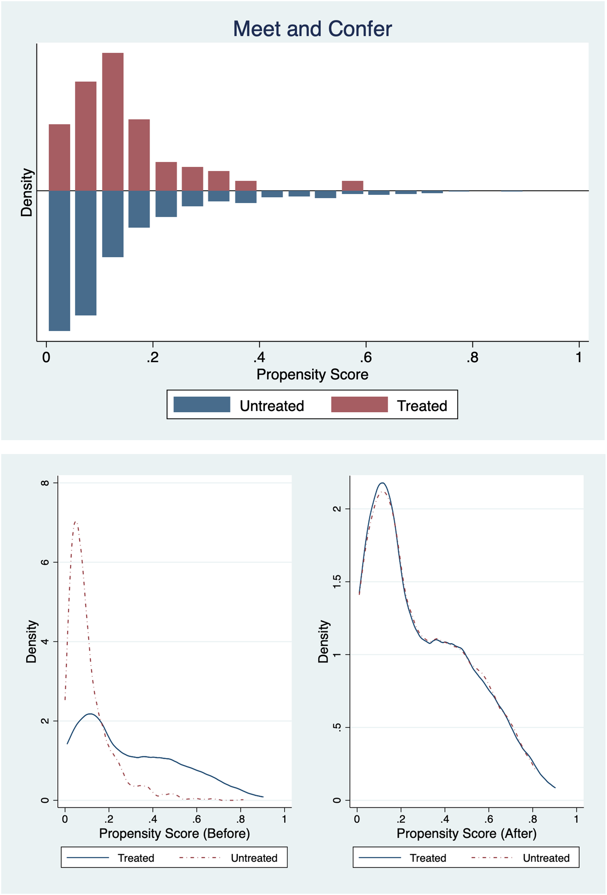
Tests for quality of the matching for union effects. (a) Histogram of Propensity Score for Meet-and-Confer (MC) status. (b) Propensity Score Distribution for MC before and after matching, by Group.

To further demonstrate the quality of the matching, we also plot the distribution of the propensity score for treated and untreated before and after the matching in Figure 4(b). It shows a significant improvement in the post-matching propensity score, attesting that the matching is successful and that our results are based on highly comparable treated and control groups.

We also employ PSM using the union density of each district, considering union density as a continuous measure of treatment. To implement this, we use the generalized propensity score (GPS) method for the continuous variable, developed by Hirano and Imbens (2004).⁹

To implement the GPS method, we first estimate the GPS, r(t, x), which is the conditional density of the actual treatment given the observed covariates, by maximum likelihood. The covariates for PSM of union density are the same variables used to estimate the propensity score for MC. For the treatment value of union density, we divide the range of union density into three treatment intervals: [0–0.26], (0.26–0.79], and (0.79–1], where 0.26 is the 10th percentile and 0.79 is the 75th percentile. Second, we estimate the conditional expectation of the outcome as a function of the two variables, treatment level (T) and GPS (R) with polynomial approximations, so that β(t, r) = E(Y|T = t, R = r). The last step is to estimate the “dose–response” function, μ(t) = E[β{t, r(t, X)}], t ∈T, by taking the average of the estimated regression function of the outcome variables over the GPS function evaluated at the desired level of the treatment. For the treatment levels of union density, we focus on the values of 0.1, 0.2, 0.3, …, 0.9, 1. We use bootstrapping to estimate the standard errors of the dose–response function.

We perform the difference-in-mean test (t-test) for all covariates in each treatment interval of union density before and after the matching to ensure that the balancing property is satisfied. Figure 5 illustrates the estimated dose–response function and estimated treatment-effect function, along with their 95% confidence bands, for one of the dependent variables: salary schedule for teachers with MA and 10 years of experience.

Figure 5.

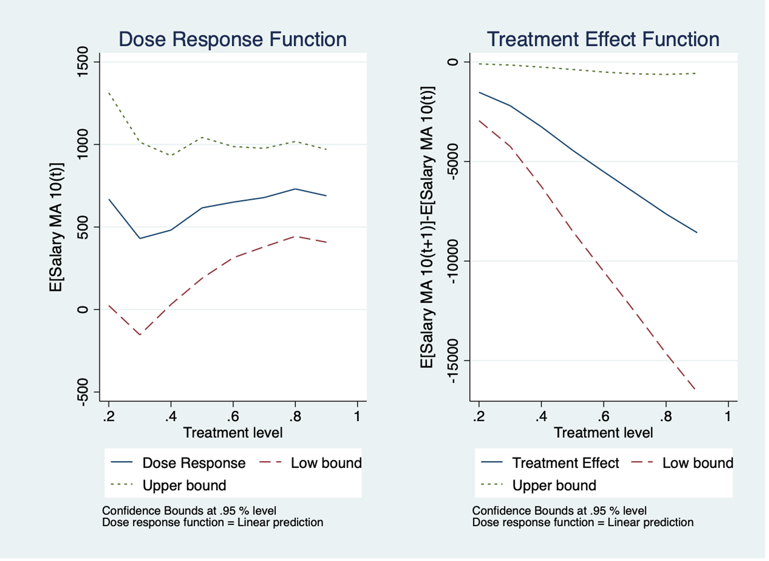
Dose–response and treatment effect function for union density.

Results

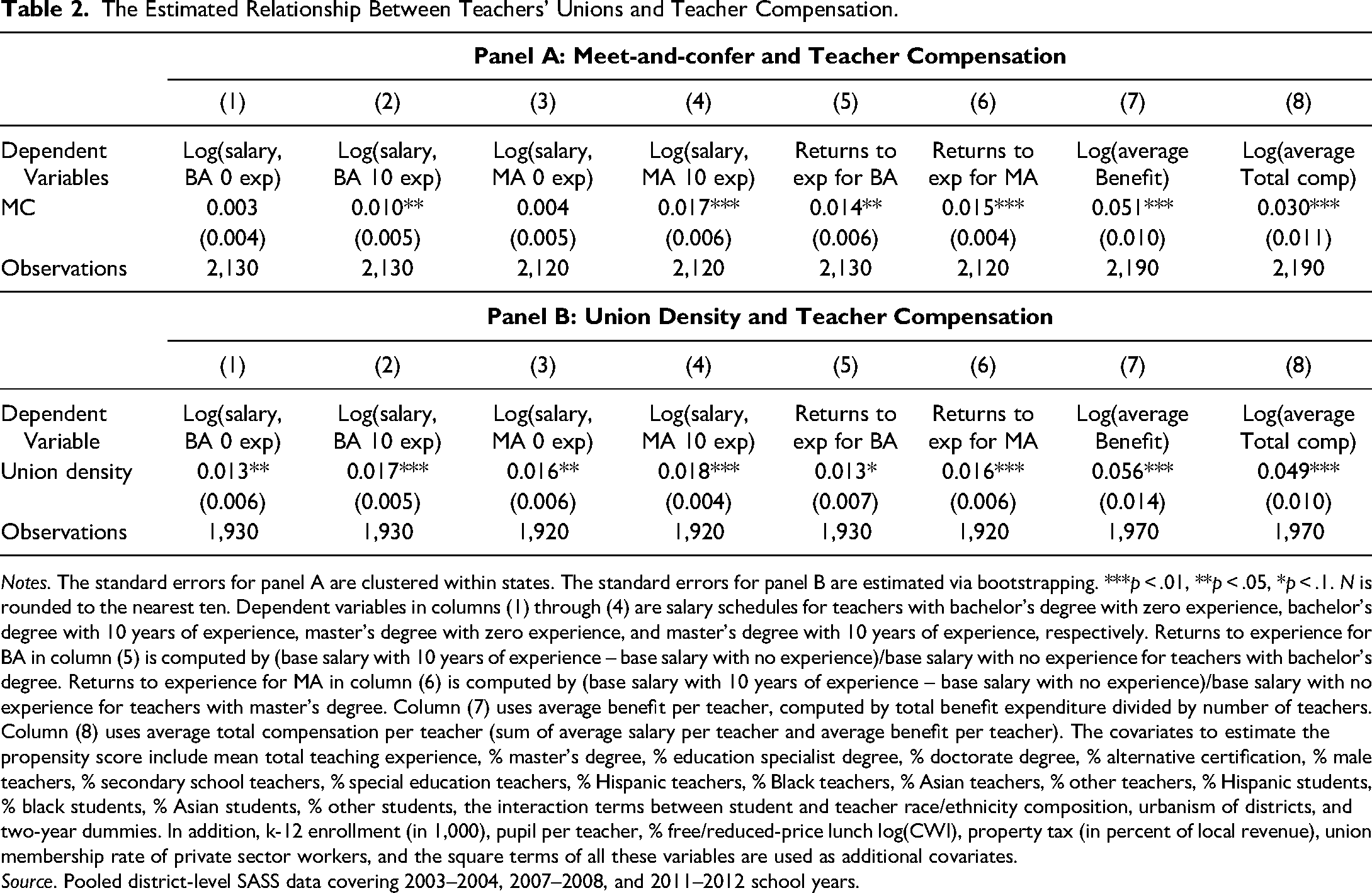
Table 2 presents the relationship between teachers’ unions and teacher pay, estimated from the PSM based on district-level data. Panel A reports the results when MC is used to measure union strength and Panel B when union density is used. Columns (1) through (4) in both panels use salary schedules for teachers with specified education level and teaching experience as dependent variables. Returns to 10 years of experience for teachers with BA and for teachers with MA are presented in columns (5) and (6), respectively. Column (7) uses the average benefit per teacher, and column (8) uses the average total compensation per teacher.

Table 2.

The Estimated Relationship Between Teachers’ Unions and Teacher Compensation.

	Panel A: Meet-and-confer and Teacher Compensation
	(1)	(2)	(3)	(4)	(5)	(6)	(7)	(8)
Dependent Variables	Log(salary, BA 0 exp)	Log(salary, BA 10 exp)	Log(salary, MA 0 exp)	Log(salary, MA 10 exp)	Returns to exp for BA	Returns to exp for MA	Log(average Benefit)	Log(average Total comp)
MC	0.003	0.010**	0.004	0.017***	0.014**	0.015***	0.051***	0.030***
	(0.004)	(0.005)	(0.005)	(0.006)	(0.006)	(0.004)	(0.010)	(0.011)
Observations	2,130	2,130	2,120	2,120	2,130	2,120	2,190	2,190
	Panel B: Union Density and Teacher Compensation
	(1)	(2)	(3)	(4)	(5)	(6)	(7)	(8)
Dependent Variable	Log(salary, BA 0 exp)	Log(salary, BA 10 exp)	Log(salary, MA 0 exp)	Log(salary, MA 10 exp)	Returns to exp for BA	Returns to exp for MA	Log(average Benefit)	Log(average Total comp)
Union density	0.013**	0.017***	0.016**	0.018***	0.013*	0.016***	0.056***	0.049***
	(0.006)	(0.005)	(0.006)	(0.004)	(0.007)	(0.006)	(0.014)	(0.010)
Observations	1,930	1,930	1,920	1,920	1,930	1,920	1,970	1,970

Notes. The standard errors for panel A are clustered within states. The standard errors for panel B are estimated via bootstrapping. ***p < .01, **p < .05, *p < .1. N is rounded to the nearest ten. Dependent variables in columns (1) through (4) are salary schedules for teachers with bachelor's degree with zero experience, bachelor's degree with 10 years of experience, master's degree with zero experience, and master's degree with 10 years of experience, respectively. Returns to experience for BA in column (5) is computed by (base salary with 10 years of experience – base salary with no experience)/base salary with no experience for teachers with bachelor's degree. Returns to experience for MA in column (6) is computed by (base salary with 10 years of experience – base salary with no experience)/base salary with no experience for teachers with master's degree. Column (7) uses average benefit per teacher, computed by total benefit expenditure divided by number of teachers. Column (8) uses average total compensation per teacher (sum of average salary per teacher and average benefit per teacher). The covariates to estimate the propensity score include mean total teaching experience, % master's degree, % education specialist degree, % doctorate degree, % alternative certification, % male teachers, % secondary school teachers, % special education teachers, % Hispanic teachers, % Black teachers, % Asian teachers, % other teachers, % Hispanic students, % black students, % Asian students, % other students, the interaction terms between student and teacher race/ethnicity composition, urbanism of districts, and two-year dummies. In addition, k-12 enrollment (in 1,000), pupil per teacher, % free/reduced-price lunch log(CWI), property tax (in percent of local revenue), union membership rate of private sector workers, and the square terms of all these variables are used as additional covariates.

Source. Pooled district-level SASS data covering 2003–2004, 2007–2008, and 2011–2012 school years.

Compared to NA districts, MC districts offer higher salary schedules with 10 years of experience for teachers with BA and teachers with MA by 1% and 1.7%, respectively. This leads to a significantly positive association between MC and returns to 10 years of experience, as MC adds 1.4% and 1.5% returns to experience for BA and MA teachers, respectively. These findings show that MC districts offer greater compensation for teachers with more experience and higher education. In MC districts, compared to NA districts, average teacher benefits and total compensation are also significantly higher by 5.1% and 3.0%, respectively.

Union density shows a small but significantly positive association with teacher salary schedules at all levels. A 10% increase in union density raises teacher salary schedules for novice teachers with BA and MA by 0.13% and 0.17%, respectively. A 10% increase in union density raises teacher salary schedules with 10 years of experience for teachers with BA and teachers with MA by 0.16% and 0.18%, respectively. Returns to experience are also appreciably higher in districts with greater union membership rates. Highly unionized districts offer greater teacher benefits and total compensation. A 10% increase in union density raises average teacher benefits and the average teacher's total compensation by 0.56% and 0.49%, respectively.

Table 3 presents the results for teachers’ employment conditions. In panel A, MC significantly improves employment conditions by reducing class size by 9%, increasing the likelihood of rewarding teachers for retaining NBPTS by 8%, and shortening school days by 0.8%. In addition, teachers report greater control in their classrooms and higher morale in the MC districts than in the NA districts. Panel B presents that union density also shows similar results as the MC cases.

Table 3.

The Estimated Relationship Between Teachers’ Unions and Employment Conditions of Teachers.

	Panel A: Meet-and-confer and Employment Conditions
	(1)	(2)	(3)	(4)	(5)
Dependent Variables	Log(pupil per teacher)	Reward NBPTS	Log(school days)	Control factor	Morale factor
MC	−0.087***	0.082***	−0.008**	0.076**	0.188**
	(0.020)	(0.022)	(0.004)	(0.032)	(0.65)
Observations	2,190	2,190	2,190	17,420	17,420
	Panel B: Union Density and Employment Conditions
	(1)	(2)	(3)	(4)	(5)
Dependent Variable	Log(pupil per teacher)	Reward NBPTS	Log(school days)	Control factor	Morale factor
Union density	−0.071**	0.013	−0.006***	0.080**	0.068*
	(0.032)	(0.008)	(0.001)	(0.032)	(0.036)
Observations	1,970	1,970	1,970	17,420	17,420

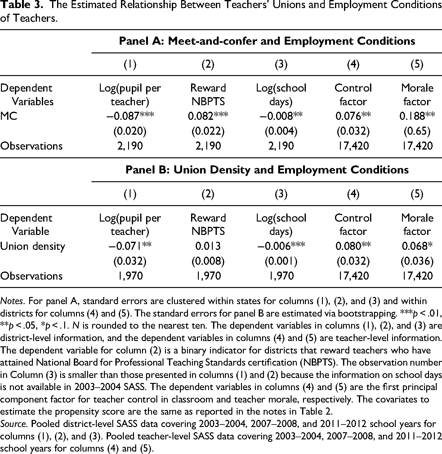
Notes. For panel A, standard errors are clustered within states for columns (1), (2), and (3) and within districts for columns (4) and (5). The standard errors for panel B are estimated via bootstrapping. ***p < .01, **p < .05, *p < .1. N is rounded to the nearest ten. The dependent variables in columns (1), (2), and (3) are district-level information, and the dependent variables in columns (4) and (5) are teacher-level information. The dependent variable for column (2) is a binary indicator for districts that reward teachers who have attained National Board for Professional Teaching Standards certification (NBPTS). The observation number in Column (3) is smaller than those presented in columns (1) and (2) because the information on school days is not available in 2003–2004 SASS. The dependent variables in columns (4) and (5) are the first principal component factor for teacher control in classroom and teacher morale, respectively. The covariates to estimate the propensity score are the same as reported in the notes in Table 2.

Source. Pooled district-level SASS data covering 2003–2004, 2007–2008, and 2011–2012 school years for columns (1), (2), and (3). Pooled teacher-level SASS data covering 2003–2004, 2007–2008, and 2011–2012 school years for columns (4) and (5).

As a sensitivity analysis, we narrow to five states that have for decades legislatively banned CB of teachers by statute: Arizona, Georgia, North Carolina, Texas, and Virginia. The alternative results are similar to those of the eight states in Tables 2 and 3.

Our findings are shown in Tables 2 and 3 suggest that districts pay their teachers significantly more and provide favorable working conditions if their unions are strong, even when a bargaining contract is not available.

How would higher pay and more favorable employment conditions translate into educational outcomes in those states? We now explore teacher turnover as a potential mechanism through which unions ultimately influence teacher quality. On one hand, if the impact of teachers’ unions on employment conditions is strong enough so that highly unionized districts would be able to attract, hire, and retain high-quality teachers, the average quality of teachers is likely to be higher in those districts than in nonunion districts. On the other hand, if unions make no impact on teacher turnover, even though teachers are better off in the districts with strong unions due to higher pay and favorable employment conditions, there may be no difference in teacher quality between less unionized and highly unionized districts.

Table 4 presents the results for the relationship between unions and teacher attrition. Odd-numbered columns present the results for all teachers. Both measures of unionization show small but statistically significantly negative associations with teacher attrition. MC is predicted to significantly reduce teachers’ attrition rate by 0.4%. A 10% increase in union density drops the attrition rate by 0.05%, but this is not statistically significantly different from zero.

Table 4.

The Estimated Relationship Between Teachers’ Unions and Teacher Attrition.

	Panel A: Meet-and-Confer		Panel B: Union Density
	(1)	(2)	(3)	(4)
	All teachers	HQT only	All teachers	HQT only
Voluntary quit	−0.0041**	−0.0083**	−0.0051	−0.0062*
	(0.0020)	(0.0039)	(0.0036)	(0.0033)
Observations	10,270	7,940	10,270	7,940

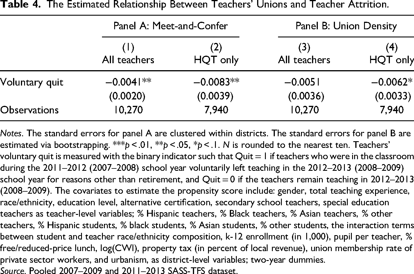
Notes. The standard errors for panel A are clustered within districts. The standard errors for panel B are estimated via bootstrapping. ***p < .01, **p < .05, *p < .1. N is rounded to the nearest ten. Teachers’ voluntary quit is measured with the binary indicator such that Quit = 1 if teachers who were in the classroom during the 2011–2012 (2007–2008) school year voluntarily left teaching in the 2012–2013 (2008–2009) school year for reasons other than retirement, and Quit = 0 if the teachers remain teaching in 2012–2013 (2008–2009). The covariates to estimate the propensity score include: gender, total teaching experience, race/ethnicity, education level, alternative certification, secondary school teachers, special education teachers as teacher-level variables; % Hispanic teachers, % Black teachers, % Asian teachers, % other teachers, % Hispanic students, % black students, % Asian students, % other students, the interaction terms between student and teacher race/ethnicity composition, k-12 enrollment (in 1,000), pupil per teacher, % free/reduced-price lunch, log(CWI), property tax (in percent of local revenue), union membership rate of private sector workers, and urbanism, as district-level variables; two-year dummies.

Source. Pooled 2007–2009 and 2011–2013 SASS-TFS dataset.

Not all teachers who voluntarily quit may be high quality. Teachers who find that teaching is not a good match may quit, which may improve educational outcomes. To address this issue, we limit our samples to teachers certified with HQT and redo the analysis. We present the results in the even-numbered columns in Table 4. Both MC and union density are statistically negatively associated with the attrition of HQT, and the magnitude of this association is appreciably greater for HQT teachers than for all teachers’ samples.

Critics of teachers’ unions claim that unions overprotect the job security of underperforming teachers (Moe 2011). However, there are several reasons why this may not be true. Schools can set higher standards for teacher recruitment and tenure because unionized districts offer better compensation and employment conditions. Also, the higher compensation unions negotiate for teachers may provide economic incentives to districts to dismiss underperforming teachers before they become extremely difficult to remove, post-tenure. Moreover, due to decreasing returns to investment on a given teacher (i.e., teachers become more costly through their careers but their productivities do not rise accordingly), districts may be more inclined to dismiss poor-performing teachers during probationary periods. Building on Han (2020), who shows that teachers’ unions are associated with greater teacher dismissal due to poor performance when exploiting national data, we examine if we can establish the same relationship in Southern states, where union strength is weaker than the national average.

Table 5 summarizes the relationship between teachers’ unions and teacher dismissal. Panel A reports the results for MC and Panel B for union density on teacher dismissal for nontenured and tenured teachers, separately. Odd-numbered columns, presenting the results for all districts, show that teachers’ unions have a significantly positive association with the dismissal of underperforming nontenured teachers. On average, compared to NA districts, MC districts have higher dismissal rates of poor-performing nontenured teachers by 6.2 percent. A 10% increase in the union density of public school teachers is associated with a higher dismissal rate of nontenured teachers by 1.25%.

Table 5.

The Estimated Relationship Between Teachers’ Unions and Teacher Dismissal Rate.

	Panel A: Meet-and-Confer and Teacher Dismissal Rate
	Non-tenured teachers		Tenured teachers
	(1)	(2)	(3)	(4)
Variable	All districts	Districts with Non-zero dismissal	All districts	Districts with Non-zero dismissal
Meet-and-Confer	0.062**	0.112***	−0.055	−0.110
	(0.032)	(0.043)	(0.058)	(0.088)
Observations	1,810	1,090	1,810	1,090
	Panel B: Union Density and Teacher Dismissal Rate
	Non-tenured teachers		Tenured teachers
	(1)	(2)	(3)	(4)
Variable	All districts	Districts with Non-zero dismissal	All districts	Districts with Non-zero dismissal
Union Density	0.125**	0.148**	−0.048	−0.099
	(0.046)	(0.060)	(0.066)	(0.098)
Observations	1,630	990	1,630	990

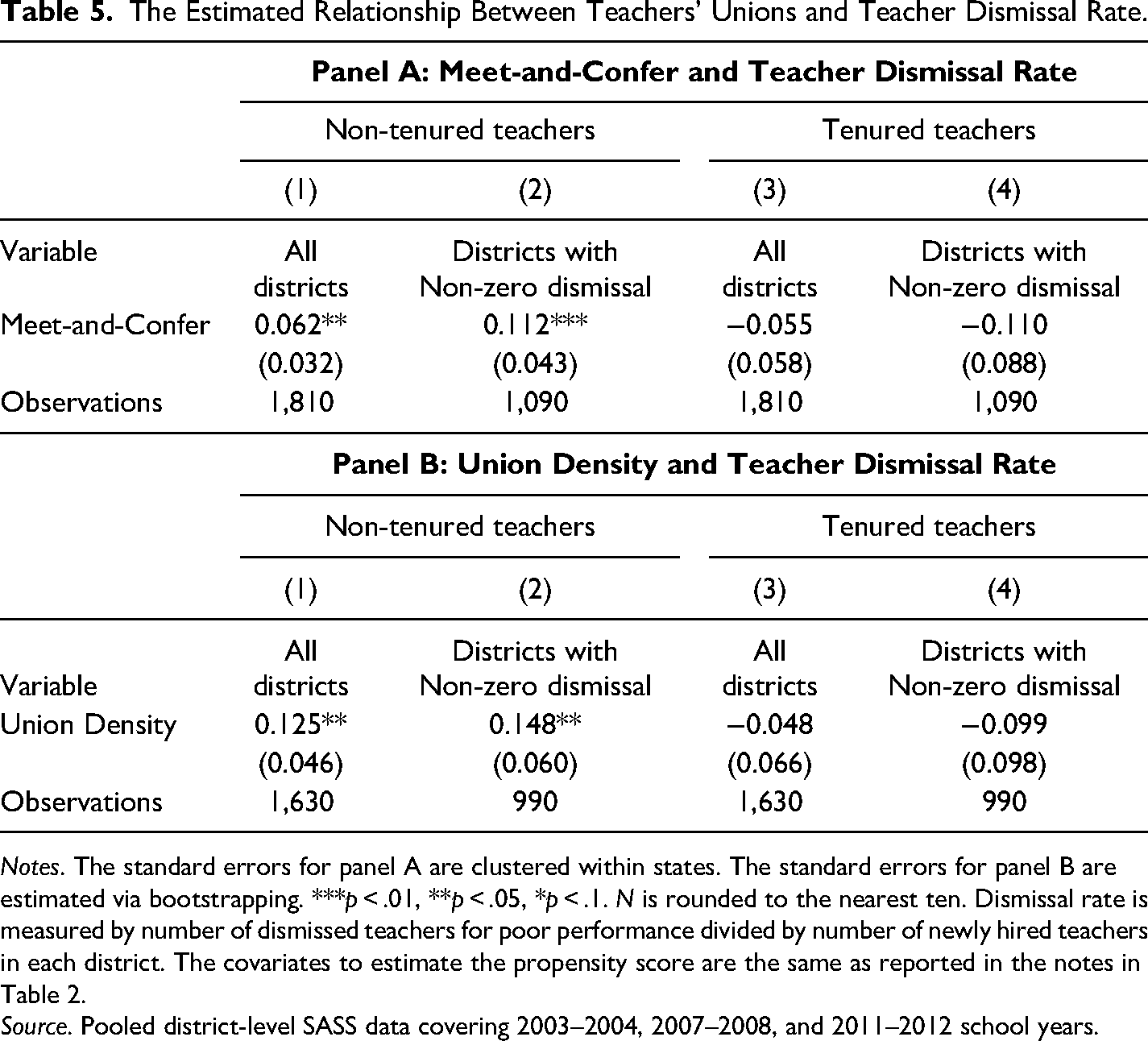
Notes. The standard errors for panel A are clustered within states. The standard errors for panel B are estimated via bootstrapping. ***p < .01, **p < .05, *p < .1. N is rounded to the nearest ten. Dismissal rate is measured by number of dismissed teachers for poor performance divided by number of newly hired teachers in each district. The covariates to estimate the propensity score are the same as reported in the notes in Table 2.

Source. Pooled district-level SASS data covering 2003–2004, 2007–2008, and 2011–2012 school years.

Many districts report zero dismissal incidence of poor-performing teachers. Districts with nonzero dismissal and districts with zero dismissal may operate differently in terms of the quality control of their teachers. Thus, we reestimate the dismissal equations only for districts with nonzero dismissal. Even-numbered columns in both panels A and B in Table 5 present the results, offering evidence of union effects on the intensive margin (in addition to the extensive margin reported in odd-numbered columns). The estimated relationship between unions and the dismissal of nontenured teachers in these districts is appreciably greater in magnitude than that presented in column (1). This indicates that union effects are greater among districts that utilize a formal process of dismissing underperforming teachers during probationary periods.

Schools with stronger teachers’ unions may dismiss more nontenured teachers during probationary periods to better protect the job security of tenured teachers. We find no evidence, however, to support such a claim. All our estimates show that the relationship between unions and the dismissal of tenured teachers is not statistically significantly different from zero.

Although states set the probation length, some states allow districts to determine the actual period, and teachers’ unions can bargain for shorter probationary periods (Brunner and Imazeki 2010). Longer probationary periods can mechanically increase the number of dismissals of nontenured teachers. As a robustness check, we use the length of probationary periods, ranging from 1 to 5 years, as an additional covariate. We also use it as another covariate for whether a district rewards teachers with NBPTS certification because schools with stronger teachers’ unions impose higher standards for teachers, which is potentially associated with teacher dismissal incidence. The alternative results remain almost the same.

As a sensitivity analysis, we measure teacher dismissal using two other metrics: the number of dismissed teachers in each district and a ratio of the number of dismissed teachers to a total number of teachers. The alternative results show a similar pattern to those presented in Table 5. MC districts and districts with higher union density dismiss more teachers for poor performance during probationary periods. Tenured teachers’ dismissal shows no relationship with teacher unionization.

We conduct an additional sensitivity test by re-doing our analysis with the five states (AZ, GA, NC, TX, and VA) that banned CB of teachers by statute. The pattern of the new results is similar to what we presented with the eight states, and, in many cases, the coefficients show greater magnitudes, indicating the greater impact of unions on teacher dismissal.

As an additional robustness test for teacher turnover, we use districts’ total revenue as a covariate. The alternative results are very similar to those presented in Tables 4 and 5, suggesting that the relationship between unions and teacher turnover does not depend on districts’ financial status in these states without CB contracts.

We also run OLS regression to check whether our results are robust to a different set of covariates. We first start by estimating the OLS model that only includes the treatment indicator (either MC or union density), and then slowly adds more control variables to the model. The coefficients on the treatment indicator in the univariate regressions are quite robust to the inclusion of various control variables, although the magnitudes of the coefficients decrease (toward zero) in most cases. Appendix V reports the summarized OLS results for all the dependent variables in Tables A1 through A4, which have the same format and the same set of covariates used in Tables 2 through 5. The OLS estimators are very similar, both quantitatively and qualitatively, to the PSM results, suggesting that our estimates based on the PSM are not sensitive to different model specifications or covariates.

The PSM reduces the bias generated by observable confounding factors, so one may question whether these results are robust to unobservable factors that may influence selection into the treatment. Thus, we conduct the sensitivity analysis proposed by Rosenbaum (2002) to check how strongly the hidden biases might affect our PSM results based on the MC treatment. The minimum Rosenbaum bound for our PSM estimators is around 1.5–1.8. This implies that unobserved characteristics would have to increase the odds ratio by less than 50–80% before they would bias the estimated impact based on the PSM. Although this value is not trivial, it does suggest that the outcomes are not immune to the potential impact of unobservable factors.

Discussion and Conclusion

In this study, we examine the relationship between teachers’ unions and teacher pay, employment conditions, and turnover in US states that do not allow bargaining contracts for public school teachers, using both district-level data and district-teacher-matched data. We measure union strength by MC status and the union membership rate of teachers. To address potential selection bias, we employ PSM using various covariates including community characteristics, such as districts’ total revenue, property tax (in percent of local revenue), union membership rate of private sector workers, cost of living, and urbanism of districts.

We find that teachers’ unions are associated with higher teacher compensation, both salaries and benefits, even when they have no bargaining rights. For instance, compared to NA districts, MC districts offer higher salary schedules for teachers with MA and 10 years of experience by 1.7% and higher average teacher benefits by 5.1%. Union density shows a significantly positive association with teacher salary schedules at all levels of teacher salary schedule. Additionally, unions significantly improve teachers’ working conditions. MC reduces class size by 9%, increases the likelihood of rewarding teachers for retaining NBPTS by 8%, shortens the number of school days by 0.8%, provides teachers with greater control in their classrooms, and raises teacher morale. Union density also shows similar results.

We also find that teachers’ unions have a significant association with teacher turnover. Both MC and union density consistently show a negative relationship with teachers’ attrition. Unionization is also predicted to increase the dismissal rate of underperforming nontenured teachers during probationary periods. For instance, compared to NA districts, MC districts have higher dismissal rates of poor-performing nontenured teachers by 6.2 percent.

We cannot claim that we have controlled for all the factors, both observable and unobservable, relevant to teachers’ unionization and their outcomes. Thus, our results should not be interpreted as evidence that teachers’ unions cause higher pay and improved working conditions in states that prohibit CB. However, with the inclusion of these additional community characteristics, we believe that the potential omitted variable bias in our results will be very small, and our estimates lean more toward causal evidence than those obtained in much of the prior work. Better study design with stronger identification is certainly an avenue for future research.

Teachers’ unions in many districts in these states may serve more as a social gathering or political lobbying group, rather than a formal representative of teachers that negotiates with districts for better terms and conditions of employment. This may be why we observe a more significant and stronger relation between unions and employment outcomes when we measure union strength with MC status, rather than with union density. MC offers a more formal channel for discussion and agreement about teacher wage steps and lanes between unions and districts. Thus, teachers’ unions in these states may find it advantageous to establish MC with their districts for obtaining better employment conditions.

In the discussion on the functions of unions in the US public sector, bargaining rights tend to be at the center of the debate. However, our study shows that teachers’ unions still organize without formal labor-management institutions and make a significant impact on teachers’ work lives, even in a hostile legal environment toward unions, shedding light on why many teachers decide to join unions in these states.

This study offers a fresh perspective beyond the frame of the “monopoly effect” of unions. We also show that union voice extends even when bargaining contracts are unavailable. The findings of this study provide evidence that teachers’ unions can enhance the efficiency of the educational system without bargaining power, as they can help in attracting and retaining higher quality teachers, through high pay and more favorable employment conditions. More frequent dismissals of underperforming probationary teachers along with lower attrition of qualified teachers in highly unionized districts are also likely to contribute to superior educational outcomes. Therefore, this study demonstrates that unions will not only benefit teachers but also enhance the effectiveness of public education.

Supplemental Material

sj-docx-1-lsj-10.1177_0160449X231164188 - Supplemental material for What Teachers’ Unions Do for Teachers When Collective Bargaining is Prohibited

Supplemental material, sj-docx-1-lsj-10.1177_0160449X231164188 for What Teachers’ Unions Do for Teachers When Collective Bargaining is Prohibited by Eunice S. Han and Jeffrey Keefe in Labor Studies Journal

Footnotes

Acknowledgments

The authors thank the National Bureau of Economic Research (NBER) for providing us with the necessary facilities and assistance. The authors also thank the National Center for Education Statistics (NCES) for kindly providing us with the data. The views expressed herein are our own and do not necessarily reflect the views of the NBER or the NCES.

Declaration of Conflicting Interests

The author(s) declared no potential conflicts of interest with respect to the research, authorship, and/or publication of this article.

Funding

The author(s) received no financial support for the research, authorship, and/or publication of this article.

ORCID iD

Eunice S. Han

Supplemental Material

Supplemental material for this article is available online.

Notes

Author Biographies

Eunice S. Han is an assistant professor at the University of Utah, a senior research associate at the Labor and Worklife Program at Harvard Law School, and a research associate at Economic Policy Institute. Han's recent research focuses on the impact of unionism on the local labor market, especially on income inequality and on economic mobility.

Jeffrey Keefe is Professor Emeritus of Labor and Employment Relations at the School of Management and Labor Relations, Rutgers University, where he has conducted research on labor markets, human resources, and labor-management relations to inform policy. Keefe is a research associate at Economic Policy Institute.

References

Abadie

Alberto

Guido W

Imbens,

. 2008. “On the Failure of the Bootstrap for Matching Estimators.” Econometrica 76 (6): 1537-1557.

Addison

John

Belfield

Clive R.

. 2004. “Union Voice.” Journal of Labor Research 25 (4): 564-96.

Barling

Julian

Fullagar

Clive

Kelloway

Kevin

. 1992. The Union and Its Members: A Psychological Approach. New York: Oxford University Press.

Batt

Rosemary

Colvin

Alexander

Keefe

Jeffrey

. 2002. “Employee Voice, Human Resource Practices, and Quit Rates: Evidence from the Telecommunications Industry.” Industrial and Labor Relations Review 55: 573-94.

Baugh

William H.

Stone

Joe A.

. 1982. “Teachers, Unions, and Wages in the 1970s: Unionism Now Pays.” Industrial & Labor Relations Review 35 (3): 368-76.

Bia

Michela

Mattei

Alessandra

. 2008. “A Stata Package for the Estimation of the Dose–Response Function Through Adjustment for the Generalized Propensity Score.” The Stata Journal: Promoting Communications on Statistics and Stata 8 (3): 354-73.

Bridges

Edwin M

. 1986. The Incompetent Teacher: The Challenge and the Response. Philadelphia: The Falmer Press.

Brunner

Eric

Hyman

Joshua

Andrew

. 2020. “School Finance Reforms, Teachers’ Unions, and the Allocation of School Resources.” The Review of Economics and Statistics 102 (3): 473-89.

Brunner

Eric

Imazeki

Jennifer

. 2010. “Probation Length and Teacher Salaries: Does Waiting Pay Off?” Industrial And Labor Relations Review 64 (1): 164-80.

10.

Brunner

Eric

Squires

Tim

. 2013. “The Bargaining Power of Teachers’ Unions and the Allocation of School Resources.” Journal of Urban Economics 76: 15-27.

11.

Cole

Stephen

. 1969. The Unionization of Teachers: A Case Study of the UFT. New York: Praeger Publishers.

12.

Cook

Jason

Lavertu

Stéphane

Miller

Corbin

. 2021. “Rent-Seeking Through Collective Bargaining: Teachers Unions and Education Production.” Economics of Education Review 85: 102193. https://doi.org/10.1016/j.econedurev.2021.102193

13.

Delaney

John T.

1985. “Unionism, Bargaining Spillovers, and Teacher Compensation.” In Advances in Industrial Relations, vol. 2, edited by Lipsky

David B.

, 111-42. Greenwich, CT: JAI Press.

14.

Demsetz

Rebecca S.

1993. “Voting Behavior in Union Representation Elections: The Influence of Skill Homogeneity and Skill Group Size.” Industrial and Labor Relations Review 47: 99-113.

15.

Eberts

Randall W.

Stone

Joe A.

. 1987. “Teachers Unions and the Productivity of Public Schools.” Industrial and Labor Relations Review 40: 354-63.

16.

Finger

Leslie K.

2018b. “Interest Group Influence and the Two Faces of Power.” American Politics Research 47 (4): 852-86.

17.

Finger

Leslie K.

2018a. “Vested Interests and the Diffusion of Education Reform Across The States.” Policy Studies Journal 46: 378-401.

18.

Frandsen

Brigham R.

2016. “The Effects of CB Rights on Public Employee Compensation: Evidence from Teachers, Fire Fighters, and Police.” Industrial & Labor Relations Review 69 (1): 84-112.

19.

Freeman

Richard B.

1980. “The Exit-Voice Tradeoff in the Labor Market: Unionism, Job Tenure, Quits, and Separations.” The Quarterly Journal of Economics 94 (4): 643-73.

20.

Freeman

Richard B.

1984. “Longitudinal Analyses of the Effects of Trade Unions.” Journal of Labor Economics 2 (1): 1-26.

21.

Freeman

Richard B.

1985. “Unions, Pensions, and Union Pension Funds.” In Pensions, Labor, and Individual Choice, edited by Wise

David A.

, 89-121. Chicago: University of Chicago Press.

22.

Freeman

Richard B.

Han

Eunice S.

. 2013. “Public Sector Unionism Without Collective Bargaining.” Paper presented at the American Economic Association (AEA) Annual Meeting, San Diego, CA, January 6, 2013. Cited in the Council of Economic Advisers Issue Brief. October 2015. http://www.aeaweb.org/aea/2013conference/program/retrieve.php?pdfid=326.

23.

Freeman

Richard B.

Medoff

James L.

. 1984. What Do Unions Do? New York: Basic Books.

24.

Goodlad

John I

. 1984. A Place Called School. Prospects for the Future. St. Louis: McGraw-Hill.

25.

Gunderson

Morley

. 2015. “Two Faces of Union Voice in the Public Sector.” Journal of Labor Research 26: 393-413. https://doi.org/10.1007/s12122-005-1012-6.

26.

Han

Eunice S.

2019. “The Impact of Teachers Unions on Teachers’ Well-Being Under Different Legal Institutions: Evidence from District-Teacher Matched Data.” AERA Open 5 (3): 233285841986729. https://doi.org/10.1177/2332858419867291.

27.

Han

Eunice S.

2020. “The Myth of Unions’ Overprotection of Bad Teachers: Evidence from District-Teacher Matched Panel Data on Teacher Turnover.” Industrial Relations 59 (2): 316-52. https://doi.org/10.1111/irel.12256.

28.

Han

Eunice S.

Keefe

Jeffrey

. 2020. “Teachers’ Unions: Engaging Teachers and Improving Student Achievement in States That Prohibit Collective Bargaining.” Educational Policy 36 (2): 407-39. https://doi.org/10.1177/0895904820901476.

29.

Han

Eunice S.

Keefe

Jeffrey

. 2021. “Candidates for Free Riding in a Post Agency Shop Public Sector.” In Advances in Industrial and Labor Relations, edited by Lewin

David

Gollan

Paul J.

. Vol. 26, 39-72. UK: Emerald Publishing Limited.

30.

Hartney

Michael

Flavin

Patrick

. 2011. “From the Schoolhouse to the Statehouse: Teacher Union Political Activism and U.S. State Education Reform Policy.” State Politics & Policy Quarterly 11: 251-68.

31.

Hirano

Keisuke

Guido W

Imbens,

. 2004. The propensity score with continuous treatments. In Applied Bayesian Modeling and Causal Inference from Incomplete-Data Perspectives, edited by A. Gelman and X.-L. Meng, 73-84. West Sussex, England: Wiley. InterScience.

32.

Hirsch

Barry T.

Macpherson

David A.

DuMond

J. Michael

. 1997. “Workers’ Compensation Recipiency in Union and Nonunion Workplaces.” Industrial and Labor Relations Review 50 (2): 213-36.

33.

Hirsch

Barry T.

Macpherson

David A.

Winters

Jon V.

. 2011. “Teacher Salaries, State CB Laws, and Union Coverage.” Paper presented at Association for Education Finance and Policy (AEFP) Meetings, Seattle.

34.

Hom

Peter

Griffeth

Rodger

. 1995. Employee Turnover. Cincinnati: South-Western Publishing.

35.

Hoxby

Caroline M

. 1996. “How Teachers’ Unions Affect Education Production.” The Quarterly Journal of Economics 111 (3): 671-718.

36.

Imazeki

Jennifer

. 2005. “Teacher Salaries and Teacher Attrition.” Economics of Education Review 24: 431-49.

37.

Ingersoll

Richard

. 2001. “Teacher Turnover and Teacher Shortages: An Organizational Analysis.” American Educational Research Journal 38 (3): 499-534.

38.

Keefe

Jeffrey

. 2018. “Pennsylvania’s Teachers Are Undercompensated – and New Pension Legislation Will Cut Their Compensation Even More.” Economic Policy Institute, Washington, DC. Available at epi.org/138380.

39.

Lindy

Benjamin A

. 2011. “The Impact of Teacher CB Laws on Student Achievement: Evidence from a New Mexico Natural Experiment.” Yale Law Journal 120 (5): 1130-91.

40.

Lovenheim

Michael F

. 2009. “The Effect of Teachers’ Unions on Education Production: Evidence from Union Election Certifications in Three Midwestern States.” Journal of Labor Economics 27 (4): 525-87.

41.

Marianno

Bradley D.

2019. “Compared to What? Changes in Interest Group Resources and the Proposal and Adoption of State Teacher Policy.” Policy Studies Journal 48 (4): 982-1022. Online Publication. https://doi.org/10.1111/psj.12345.

42.

Marianno

Bradley D.

Bruno

Paul

Strunk

Kathrine O.

. 2021. “The Effect of Teachers’ Union Contracts on School District Efficiency: Longitudinal Evidence From California.” SAGE Open 11 (1): 215824402098868. https://doi.org/10.1177/2158244020988684.

43.

Merkle

Jessica S.

Phillips

Michelle Andrea

. 2018. “The Wage Impact of Teachers Unions: A Meta-Analysis.” Contemporary Economic Policy 36 (1): 93-115.

44.

Moe

Terry M.

2011. Special Interest. Washington D.C: Brookings Institution Press.

45.

Mueller

Charles

Price

James

. 1990. “Economic, Psychological and Sociological Determinants of Voluntary Turnover.” Journal of Behavioral Economics 19: 321-35.

46.

Murnane

Richard J.

Olson

Randy J.

. 1990. “The Effects of Salaries and Opportunity Costs on the Length of Stay in Teaching.” The Journal of Human Resources 25 (1): 106-24.

47.

Paglayan

Agustina S.

2019. “Public-Sector Unions and the Size of Government.” American Journal of Political Science 63 (1): 21-36.

48.

Podgursky

Michael J.

2003. “Fringe Benefits: There is More to Compensation Than a Teacher’s Salary.” Education Next 3 (3): 71-6.

49.

Rees

Daniel I.

1991. “Grievance Procedure Strength and Teacher Quits.” Industrial Labor Relations Review 45 (1): 31-43.

50.

Rose

Heather

Sonstelie

Jon

. 2010. “School Board Politics, School District Size, and the Bargaining Power of Teachers’ Unions.” Journal of Urban Economics 67 (3): 438-50.

51.

Rosenbaum

Paul R.

2002. Observational Studies. New York: Springer.

52.

Rosenbaum

Paul R.

Rubin

D. B.

. 1985. “Constructing a Comparison Group Using Multivariate Matched Sampling Methods That Incorporate the Propensity Score.” The American Statistician 39: 33-8.

53.

Rosenberg

Sarah

Silva

Elena

. 2012. “Trending toward Reform: Teachers Speak on Unions and the Future of the Profession.” Education Sector Reports. http://educationpolicy.air.org/sites/default/files/publications/REPORT-TeacherSurvey3f.pdf

54.

Rosenfeld

Jake

. 2010. “Economic Determinants of Voting in an Era of Union Decline.” Social Science Quarterly 91: 379-95.

55.

Rosenholtz

Susan

. 1989. Teacher’s Workplace: The Social Organization of Schools. New York: Longman.

56.

Steer

Richard M.

Mowday

Richard

. 1981. “Employee Turnover and the Post-Decision Accommodation Process.” In Research in Organizational Behavior, edited by Shaw

B. M.

Cummings

L. L.

. 235-281. Greenwich: JAI Press.

57.

Stoddard

Christiana

. 2005. “Adjusting Teacher Salaries for the Cost of Living: The Effect on Salary Comparisons and Policy Conclusions.” Economics of Education Review 24: 323-39.

58.

Taylor

Lori L.

Fowler

William J.

. 2006. “A Comparable Wage Approach to Geographic Cost Adjustment.” Washington, DC: National Center for Education Statistics.

59.

Theobald

Neil

. 1990. “An Examination of the Influence of Personal, Professional, and School District Characteristics on Public School Teacher Retention.” Economics of Education Review 9: 241-50.

60.

West

Kristine L.

2015. “Teachers’ Unions, Compensation, and Tenure.” Industrial Relations: A Journal of Economy and Society 54 (2): 294-320.

61.

Winters

John V.

2011. “Teacher Salaries and Teacher Unions: A Spatial Econometric Approach.” Industrial and Labor Relations Review 64 (4): 747-64.

62.

Zigarelli

Michael

. 1996. “Bargaining Law Provisions and Teacher Bargaining Outcomes.” Journal of Labor Research 17 (1): 135-48.

63.

Zwerling

Harris L.

Thomason

Terry

. 1995. “CB and the Determinants of Teachers’ Salaries.” Journal of Labor Research 16 (4): 467-84.

Supplementary Material

Please find the following supplemental material available below.

For Open Access articles published under a Creative Commons License, all supplemental material carries the same license as the article it is associated with.

For non-Open Access articles published, all supplemental material carries a non-exclusive license, and permission requests for re-use of supplemental material or any part of supplemental material shall be sent directly to the copyright owner as specified in the copyright notice associated with the article.

0.00 MB

0.05 MB