Using Monte Carlo simulations to determine power and sample size for planned missing designs

Abstract

Planned missing data designs allow researchers to increase the amount and quality of data collected in a single study. Unfortunately, the effect of planned missing data designs on power is not straightforward. Under certain conditions using a planned missing design will increase power, whereas in other situations using a planned missing design will decrease power. Thus, when designing a study utilizing planned missing data researchers need to perform a power analysis. In this article, we describe methods for power analysis and sample size determination for planned missing data designs using Monte Carlo simulations. We also describe a new, more efficient method of Monte Carlo power analysis, software that can be used in these approaches, and several examples of popular planned missing data designs.

Keywords

missing data analysis power analysis three-form planned missing design

Missing data is a problem almost all researchers in psychology must confront when designing studies and analyzing results. Modern missing data techniques such as full information maximum likelihood (FIML) and multiple imputation (MI) provide researchers with tools to accurately and powerfully estimate parameters in the presence of ignorable missing data (Baraldi & Enders, 2010). With these modern methods, missing data can now be incorporated into study designs allowing researchers to a priori assign participants to be missing on a proportion of responses (Graham, Taylor, Olchowski, & Cumsille, 2006). An important consideration when designing a study with a planned missing design is determining how sample size and planned missing data will affect statistical power. In this article, we discuss how to determine power and sample size requirements for studies with planned missing designs, with a specific focus on analyses conducted using Structural Equation Modeling (SEM). We first provide an overview of planned missing data designs, followed by a discussion of power analysis methods for SEM, and finally, we cover power analyses with planned missing designs, including discussion of software to implement these power analyses and several examples.

Planned missing designs

There are many types of planned missing designs, especially when data are longitudinal (e.g. cohort sequential designs, accelerated longitudinal designs). In this article, we will focus on two types of planned missing designs that can be applied to cross-sectional or longitudinal research: the three-form design and the two-method design (Graham et al., 2006). The three-form design, a form of matrix sampling, involves splitting items into four groups: X, A, B, and C. All participants complete all items in the X block, and participants are randomly assigned to complete two additional blocks. This design results in three possible forms for participants: XAB, XAC, and XBC (Table 1). The three-form design provides important benefits in data collection. With the same amount of effort, researchers can collect more data from each participant. For example, if there are 10 items in each set (X, A, B, and C), then a researcher would have data on 40 items, but each participant would only complete 30 of the possible items. When each participant is completing fewer items in a planned missing data design, participant fatigue and practice effects may be reduced. In essence, a three-form design may result in “cleaner” data (Graham et al., 2006; Rhemtulla & Little, 2012).

Table 1.

Example of three- and four-form designs.

Proportion of sample	Set X	Set A	Set B	Set C
1/3	X	X	X	O
1/3	X	X	O	X
1/3	X	O	X	X

Proportion of sample	Set X	Set A	Set B	Set C	Set D
1/4	X	X	X	O	O
1/4	X	X	O	X	O
1/4	X	O	X	O	X
1/4	X	O	O	X	X

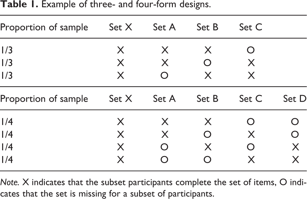
Note. X indicates that the subset participants complete the set of items, O indicates that the set is missing for a subset of participants.

The “three-form” design does not need to be limited to three subsets of missing items and three-form. Raghunathan and Grizzle (1995) proposed a design with six item sets and 10 possible forms. An important consideration when investigating multiple-form designs is that not every possible combination of sets of items must be included. In Table 1, we demonstrate how a four-form design might be arranged with each participant completing items in the X block and in 2 other blocks. There are six possible forms (XAB, XAC, XAD, XBC, XBD, XCD) but all covariances among items can be measured using only four forms (e.g., XAB, XAC, XBC, XCD). An important issue to consider when developing an n-forms design is that there must be covariance coverage for items across forms. For example, a three-form design where each participant is only assigned to one block (e.g. XA, XB, and XC) will have no covariance coverage between items in the A, B, and C blocks and across block statistics will not be estimable.

The “two-method” design can be implemented when there are two kinds of measures of the same construct: a relatively cheap, less valid measure, e.g. self-reported levels of stress, and an expensive, more valid measure, e.g. salivary cortisol (Graham, et al., 2006). By using both types of measures as indicators of the same latent variable, e.g. stress (see Figure 1), researchers can remove any bias associated with the cheap measure by borrowing more accurate information from the expensive measure and use the sample size benefit by using the cheap measure to increase the power to detect the effects of interest. This is accomplished by modeling two latent variables, the latent variable representing the construct of interest, e.g. stress, and a latent variable representing a “bias” or “method” factor, e.g. self-report bias. The latent variable representing the construct can then be used as a predictor or outcome in a larger model. One important caveat for the two-method design is that there must be multiple measures of the cheap, or biased, measure to serve as indicators of the “bias” latent variable. If there is only one measure of the cheap measure, it is impossible to model the bias related to the cheap measure. In the two-method design, planned missingness is imposed on the expensive measure: all participants complete the cheap measure, and a smaller percentage of the sample is randomly selected to also complete the expensive measure.

Figure 1.

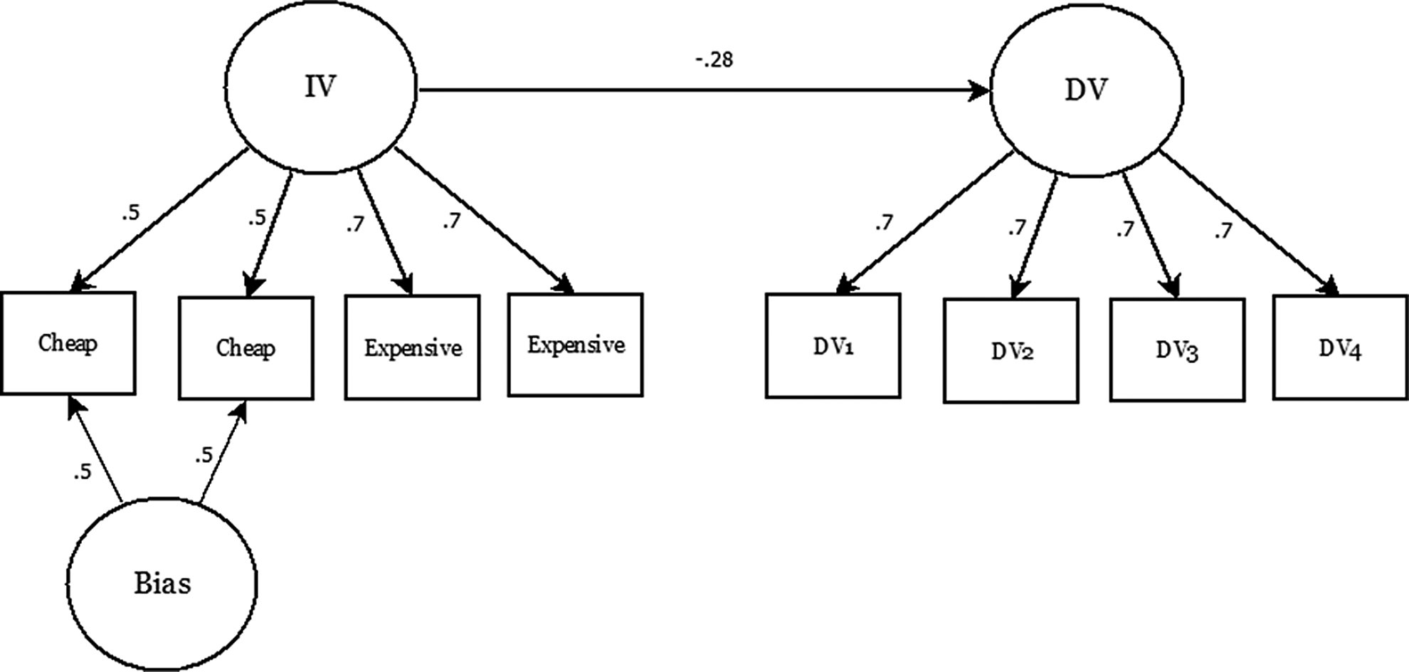
Example of a model used for two-method planned missing data design. Planned missing is imposed on the expensive measures of the IV. Adapted from Graham, Taylor, Olchowski, & Cumsille (2006), Figure 2.

Power for planned missing designs

The two types of planned missing designs can have differential effects on power: the three-form designs can reduce power whereas in some situations, and the two-method design can increase power compared to complete data designs with equal costs (Enders, 2010; Graham et al., 2006). Determining power losses in the three-form designs is based on a simple logic: the power to detect correlations between items is attenuated by missing data. The amount of attenuation increases as the percent of missing data increases. As a result, in a three-form design, the power to detect the correlation between two items in the X block will be highest (0% of data is missing), power to detect a correlation between an item in the X block and an item in the A (or B or C) block will be next highest (33% of data is missing on one variable), power to detect a correlation between two items in the A (or B or C) block will be lower (33% of data is missing on two variables), and the power to detect correlation between an item in the A block and an item in the B or C block will be lowest (33% of data is missing on two variables, and each variable is missing data for different participants).

Though the three-form design can result in loss of power, there are several mitigating factors in favor of using the three-form design. The three-form design allows researchers to investigate the relationships among more variables than a complete data design while requiring participants to fill out a survey of the same length. The three-form design can also result in each participant filling out a shorter measure, possibly resulting in less participant fatigue and unplanned missing data (Harel, Stratton, & Aseltine, 2011). Power for these designs has generally been based on the power to detect correlations within a correlation matrix (Graham et al., 2006) or in the context of regression (Raghunathan & Grizzle, 1995). There has been less work assessing power for a three-form design for latent variable models. Thus, it is not clear the degree to which implementing different planned missing data designs will affect power in this context. Researchers interested in using the three-form design are encouraged to perform an a priori power analysis to determine how implementing a three-form design will impact power specific models and sample sizes.

In contrast with the three-form design, when a researcher is working with a fixed budget, the two-method design can increase power, compared to a complete case design (Graham et al., 2006). For example, imagine that a researcher has $10,010 to spend on his or her experiment with cheap measures that cost $5 per person, and expensive measures that cost $50 per person. With a complete case design, the experimenter would have a sample size of 182 (10,010/55). For the same cost, the researcher could also assess 150 individuals on both the cheap and expensive measures and an additional, 352 individuals on the cheap measure only (150 × 55 + 352 × 5 = 10,010). In this case, about 70% of the sample has missing data on the expensive measure. Alternatively, the researcher could assess 100 individuals on both the cheap and expensive measures and an additional 902 individuals on the cheap measure only (100 × 55 + 902 × 5 = 10,010), in which case about 90% of the sample would have missing data on the expensive measure. The optimal way to allocate costs and assign planned missing data in a two-method design depends on several factors including the relative cost of the cheap and expensive measures, the reliability of each measure, and the size of the effect to be investigated. A priori power analyses allow researchers to determine the appropriate ratio of cheap to expensive measures and overall sample size (see Table 2).

Table 2.

Example of two-method design.

Proportion of Sample	Cheap	Expensive
3/4	X	O
1/4	X	X

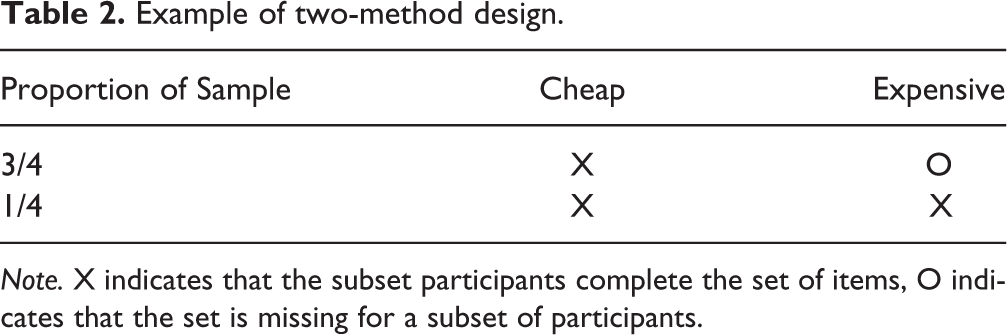
Note. X indicates that the subset participants complete the set of items, O indicates that the set is missing for a subset of participants.

Power analysis for SEM

When discussing power and sample size in SEM, there are two types of power that can be considered: 1) the power to detect if a parameter estimate(s) is significantly different from a specified value, usually zero, assuming a correctly specified model, and 2) the power to detect model misspecifications. This article will focus on power analysis to detect parameter estimates. Two methods are used for power analysis in SEM: a method based on the noncentrality parameter of the fit function (e.g. MacCallum, Browne, & Sugawara, 1996; Satorra & Saris, 1985), and a method using Monte Carlo simulations (Muthén & Muthén, 2002).

Power analysis based on the noncentrality parameter

Suppose a researcher wants to conduct a power analysis for a two factor CFA model. The purpose is to determine the sample size so that there is sufficient power to detect the correlation between the two latent factors. For example, assume the null hypothesis is that the correlation is zero in the population and the true population correlation is .1. When assessing power based on the non-centrality parameter, the researcher first computes a model implied covariance matrix based on the alternative hypothesis (i.e., a model with two latent variables correlated at .1) and then fits a model, with the correlation fixed at 0, to the covariance matrix. The obtained likelihood ratio test statistic is an estimate of the non-centrality parameter that can be used to compute the power to reject the null hypothesis. This approach has been extended to hypotheses related to model fit (MacCallum et al., 1996), nested model comparisons (MacCallum, Browne, & Cai 2006), and missing data (Davey & Savla, 2009, 2010). A detailed discussion of these methods is beyond the scope of this article. The current article is focused on the Monte Carlo approach which is a more flexible approach to power analysis and can be easily extended to planned missing data designs. In the following, we describe the Monte Carlo approach and the way to extend it to planned missing data designs using several examples. Software options for implementing the Monte Carlo approach with missing data are also discussed.

Monte Carlo approach to power analysis in SEM

The idea behind the Monte Carlo approach to power analysis is straightforward. Because power is the probability of rejecting the null hypothesis given the alternative hypothesis is true, if one can draw a large number (e.g., 1,000) of random samples from the population defined by the alternative hypothesis and fit the hypothesized model on the samples, power can be then estimated as the proportion of samples that reject the null hypothesis. The only complexity here is to draw random samples from a specified population, which is the purpose of Monte Carlo simulations. We now use the previous example to illustrate the Monte Carlo approach to power analysis. First, random samples of a specified sample size need to be drawn from the population based on the CFA model with the factor correlation equal to .1. Second, the CFA model with the correlation and other model parameters freely estimated is fit to each of the random samples. The power to detect the correlation coefficient is then estimated as the proportion of the samples that have a significant correlation coefficient. For example, if a Monte Carlo power analysis used 1,000 replications, and the correlation coefficient was significantly different from 0 in 700 of the replications, then power would be .70 for the correlation coefficient.¹ If the obtained power is less than or larger than the desirable level (.80, for example), then the sample size needs to be increased or decreased correspondingly. The entire procedure needs to be repeated until the desirable level of power is achieved.

In addition to determine the required sample size for sufficient power to detect an effect, researchers planning a study should determine the sample size to achieve accurate point and standard error estimates of an effect (Lai & Kelley, 2011). In the Monte Carlo approach, accuracy in point and standard error estimates is indicated by small relative bias in point and standard error estimates. Relative bias in point estimate for each parameter is computed by subtracting the average estimated parameter value from the population parameter value, and then dividing this value by the population parameter value. Standard error bias for each parameter is computed in a similar way, the average standard error across replications is subtracted from the population standard error (the standard deviation of the parameter estimate across replications) and this value is divided by the population standard error.

As described above, to determine an appropriate sample size for a proposed study, a researcher needs to draw many random samples under the population model with different sample sizes until he or she found the sample size that yielded the desired level of power or accuracy in point and standard error estimates. Thus, the process can sometimes become extremely tedious and time-consuming. We have developed a new method for power analysis using a Monte Carlo approach. This new method would require a researcher to run only a single Monte Carlo simulation, resulting in more efficient estimation of an appropriate sample size.

Monte Carlo power analysis with continuously varying sample size

Our new method of power analysis is based on a new approach to Monte Carlo simulations: continuously varying simulation factors. In a traditional Monte Carlo simulation, all simulation factors (model parameters, sample size (n), percent missing data) are static across all replications (e.g. all replications have the same n). Power is estimated by the proportion of significant replications and can only be computed for a single sample size at a time. In other words, one has to run the simulation again to know the power associated with another sample size. With continuously varying factors, the design factors take on a different set of values for each replication (e.g. each replication has a different n), factors can either vary randomly or increase by small increments over a range of values. In this case, each factor becomes a variable which can be used to predict power. For example, one can predict power from n using a logistic regression analysis. The estimated logistic regression equation can be then used to predict power from any sample size (within the specified range) without rerunning the simulation.

The steps for a power analysis with continuously varying n are as follows: 1) run many replications of a simulation with different n for each replication, 2) record the n and significance of parameters (0 not significant, 1 significant) for each replication, 3) for a given parameter, fit a logistic regression predicting the parameter’s significance from n, 4) compute the predicted probability of success at a given sample size, this value is an estimate of power at that sample size.

p = \frac{e^{B_{0} + B_{1} N}}{1 + e^{B_{0} + B_{1} N}}

where B₀ is the intercept of the logistic regression equation, and B₁ is the slope of sample size in the logistic regression equation.² This approach allows researchers to run a single Monte Carlo simulation (albeit one with many replications) and compute power for a specific sample size, a number of sample sizes, or plot power curves over a range of sample sizes. One important caveat to this method is that the power computed from this method is an estimate. The precision of the estimated power will depend on the total number of replications run with varying sample sizes. Thus we recommend running a simulation with many (e.g. 1,000 or more) replications to help determine power. As an additional check, after determining sample size with continuously varying sample sizes researchers may want to run another Monte Carlo power analysis with the sample size fixed to the sample size found with continuously varying sample sizes.

Monte Carlo power analysis with missing data

Incorporating missing data into Monte Carlo power analysis is a straightforward exercise. Missing data must be accounted for in both the data generation and analysis stages of a Monte Carlo simulation. In data generation, missingness must be imposed on each generated data set and the pattern of missingness can be determined by the researchers. For example, to incorporate a three-forms design in a Monte Carlo simulation with 12 variables, the first three variables will not have any missing data (the X block), the next three variables will be missing for the first third of participants (the A block), the next three variables will be missing for the second third of participants (the B block) and the final three variables will be missing for the final third of participants (the C block).³ Once data are generated with missing values, the analysis portion of each replication should appropriately handle the missing data with modern methods, either FIML, or MI. Currently, we are aware of two SEM software packages that can both simulate data for planned missing data designs, and also appropriately model the missing data with FIML or MI.

Software for conducting Monte Carlo power analyses with planned missing designs

Several computer programs have been developed to automate generating data, imposing missing data, and combining analysis results across replication in a Monte Carlo simulation. This article will discuss two available programs: Mplus (Muthén & Muthén, 1998–2013) and the R package simsem (Pornprasertmanit, Miller, & Schoemann, 2013).

Mplus

Mplus is a statistical program that aims to analyze basic and advanced structural equation modeling. Note that this review is based on Mplus version 7. Both MI and FIML methods for missing data handling are available in Mplus. Mplus provides a Monte Carlo simulation framework that can create and analyze data based on simple (e.g. confirmatory factor analysis) or advanced models (e.g. growth mixture modeling) and summarize results across multiple replications.

Missingness can be imposed on generated data sets with the MISSING and MODEL MISSING command. Users can impose different missing data patterns to the generated data using the PATMISS and PATPROBS commands. For example, the first half of the generated data can have 40% missing on the first variable but the second half can have no missing data on the first variable. These commands allow Mplus to create planned missing data, such as those from three-form design or two-method design. Additionally, planned missing data with additional (unplanned) missing can also be generated. Mplus also provides a detailed manual with many examples so that users can easily find examples for missing data generation.

However, using Mplus has some notable limitations. First, the current version of Mplus v. 7.11 does not support missingness due to dropout, or attrition. That is, if participants drop out from a study, they will not provide any information in the following time points. Additionally, at this time, Mplus does not support multiple imputation within Monte Carlo simulations. Finally, Mplus does not have any built in functionality for the Monte Carlo approach with continuously varying sample sizes.

simsem package featuring other R packages

simsem is an R package that aims to facilitate large-scale Monte Carlo simulations in a Structural Equation Modeling framework. This review is based on simsem version 0.5-3. simsem is embedded in R environment (R Core Team, 2013). Importantly, R, simsem, and other packages are free and open source. Currently, simsem can generate data, use the lavaan, (Rosseel, 2012) or OpenMx (Boker, et al., 2012) packages to analyze simulated data, and summarize results into an object, called a results object. Users can request different output from the results object with different commands, which differs from Mplus where all results are provided in a single text file. The results from a simulation can be used for further calculation or aggregation inside the R environment.

simsem is designed to impose many missing data patterns, such as MCAR, MAR, attrition, and planned missing data (including three-form and two-method designs). The available missing data patterns can be combined together so that a user could specify, for example, attrition on top of a planned missing design. Importantly, users can use a priori missing data template (a matrix representing the positions of missing values) or can write their own functions to create missing data (e.g. missing observations based on an interaction between two variables). To account for missing data, MI from different packages can be used, including the Amelia (Honaker, King, & Blackwell, 2011) and mice (van Buuren & Groothuis-Oudshoorn, 2011) packages. Alternatively, FIML can be used with the lavaan or OpenMx packages. For further details, a user-friendly vignette is available online at www.simsem.org, and more technical details are available through the official R documentation files.

One of the primary advantages of using simsem is that researchers can see the source code in the package to check how each step is implemented. However, there are some limitations in the current version of simsem. Some models are not available in simsem, such as multilevel models or growth mixture models. While multiple group models are supported, missing data patterns cannot be different across these groups. However, multiple-group missing patterns could be implemented by writing a custom R function and specifying it in the simulation facilities of simsem. Finally, some advanced features (e.g. imposing model misspecification) require users to specify matrices and vectors (using LISREL style), which may not be familiar to some users.

To illustrate how to determine power for planned missing designs with simsem, we include the following two examples (for more examples, see www.simsem.org).

Example 1: Three-form planned missing data design

In the first example, we specify a 2 factor CFA model with 9 indicators per-factor and impose a three-form planned missing design. We then calculate the sample size needed to achieve a power of .80 for the latent correlation parameter. In this example, we include a detailed, line-by-line description of the syntax for clarity which is not included in the second example. Specification of Monte Carlo simulations for structural equation models with simsem can be done using several different syntax styles, including lavaan (similar to Mplus), OpenMx, and a LISREL-style matrix notation. Using LISREL notation (Jöreskog, 1969) the covariance structure of the model is defined by four parameter matrices: Λ is a matrix of factor loadings with the number of rows equal to the number of manifest variables and the number of columns equal to the number of latent variables, Θ_ε is a covariance matrix of the measurement errors associated with indicator variables with the number of rows equal to the number of manifest variables and the number of columns equal to the number of manifest variables, Ψ is a covariance matrix of latent variables with the number of rows equal to the number of latent variables and the number of columns equal to the number of latent variables, and B is a matrix of structural relations among latent variables with the number of rows equal to the number of latent variables and the number of columns equal to the number of latent variables.⁴ The covariance structure implied by the model is:

\sum = Λ {(I - B)}^{- 1} (Ψ) {(I - B)}^{- 1'} Λ^{'} + Θ_{ε}

For the following examples with simsem, we use the LISREL-style matrix notation. Throughout, we assume a basic knowledge of R; readers interested in learning more about R are encouraged to consult one of the many excellent books dedicated to learning R (e.g. Muenchen, 2009; Verzani, 2004).

The LISREL-style matrix syntax for Monte Carlo simulations has two parts: data generation and analysis. Each part is represented by R matrices that will be joined together to form a complete matrix object using the function bind. To completely specify a CFA model requires 3 matrix objects: a factor loading matrix (LY), a factor covariance matrix (PS), and an error covariance matrix (TE), see Table 3 for an example of these matrices. For the analysis specification, elements of the matrix to be estimated are freed by assigning “NA” to that element. Elements can also be fixed to 0 or any other numerical value by assigning that value to an element in a similar way. We demonstrate this in the script in lines 2–4 with the factor loading matrix. Numbers in parentheses represent that line in the embedded R syntax.

Table 3.

Model Matrices for Example 1 with population values.

LY
.7*	0
.7*	0
.7*	0
.7*	0
.7*	0
.7*	0
.7*	0
.7*	0
.7*	0
0	.7*
0	.7*
0	.7*
0	.7*
0	.7*
0	.7*
0	.7*
0	.7*
0	.7*
PS
1	.2*
.2*	1

TE
.51*	0	0	0	0	0	0	0	0	0	0	0	0	0	0	0	0	0
0	.51*	0	0	0	0	0	0	0	0	0	0	0	0	0	0	0	0
0	0	.51*	0	0	0	0	0	0	0	0	0	0	0	0	0	0	0
0	0	0	.51*	0	0	0	0	0	0	0	0	0	0	0	0	0	0
0	0	0	0	.51*	0	0	0	0	0	0	0	0	0	0	0	0	0
0	0	0	0	0	.51*	0	0	0	0	0	0	0	0	0	0	0	0
0	0	0	0	0	0	.51*	0	0	0	0	0	0	0	0	0	0	0
0	0	0	0	0	0	0	.51*	0	0	0	0	0	0	0	0	0	0
0	0	0	0	0	0	0	0	.51*	0	0	0	0	0	0	0	0	0
0	0	0	0	0	0	0	0	0	.51*	0	0	0	0	0	0	0	0
0	0	0	0	0	0	0	0	0	0	.51*	0	0	0	0	0	0	0
0	0	0	0	0	0	0	0	0	0	0	.51*	0	0	0	0	0	0
0	0	0	0	0	0	0	0	0	0	0	0	.51*	0	0	0	0	0
0	0	0	0	0	0	0	0	0	0	0	0	0	.51*	0	0	0	0
0	0	0	0	0	0	0	0	0	0	0	0	0	0	.51*	0	0	0
0	0	0	0	0	0	0	0	0	0	0	0	0	0	0	.51*	0	0
0	0	0	0	0	0	0	0	0	0	0	0	0	0	0	0	.51*	0
0	0	0	0	0	0	0	0	0	0	0	0	0	0	0	0	0	.51*

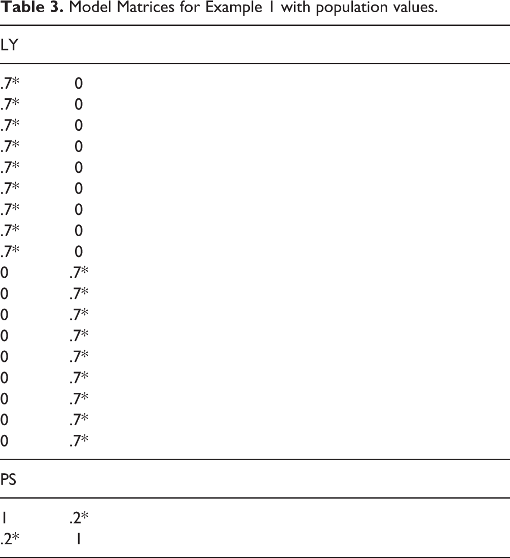
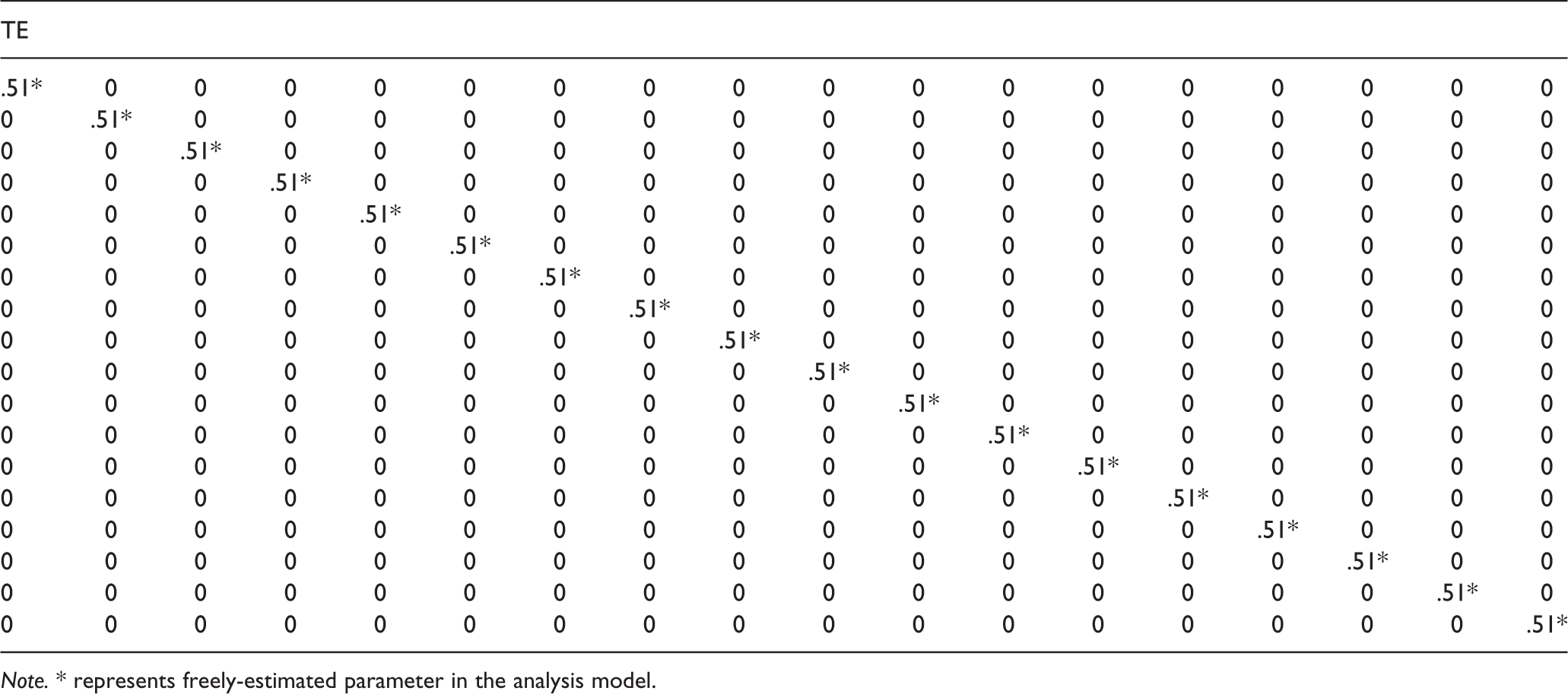
Note. * represents freely-estimated parameter in the analysis model.

1 library(simsem)

2 loading <- matrix(0, nrow=18, ncol=2)

3 loading[1:9,1] <- NA

4 loading[10:18,2] <- NA

After loading the library in line 1, we build the 18 × 2 loading matrix for analysis with 0 as the default value (2), which we have arbitrarily called “loading.” Next, we free the factor loadings for the indicators that load onto each factor: indicators 1–9 for Factor 1 in column 1 (3), and 10–18 for Factor 2 in column 2 (4).

The loading matrix for data generation specification is represented by a matrix that contains population parameters corresponding to each of the parameters freed in lines 2–4. In lines 5–7, we assign the value of .7 to the position of each freely-estimated parameter in the previous loading matrix into a matrix called “value” that has identical dimensions. In line 8, both the “loading” matrix and the “value” matrix are combined together using the function bind, creating a matrix object that will be used later to form templates for data generation and analysis.

5 value <- matrix(0, nrow=18, ncol=2)

6 value[1:9,1] <- .7

7 value[10:18,2] <- .7

8 LY <- bind(loading, value)

For the simple case where all free parameters will have the same population parameter value, a user could simply pass that value as the second argument to bind, eliminating the need to create the second “value” matrix:

LY <- bind(loading, 0.7)

We repeat this process for the factor covariance matrix object. However, instead of specifying the factor covariances (noted as “PS”), we can instead specify a matrix of factor correlations (RPS) and factor variances (VPS). If the factor variances are unspecified by the user, the program sets these variances to be fixed at 1, allowing the factor covariance parameter to be correctly interpreted directly as a correlation. In lines 9–11, we create the factor correlation matrix and set the population parameter values to .2, and use the program default for the factor variances. In this situation, because the factor correlation matrix is symmetric, we use the function binds, which simply sets the symmetric argument in bind to be true.

9 factor.cor <- matrix(NA, nrow=2, ncol=2)

10 diag(factor.cor) <- 1

11 RPS <- binds(factor.cor,.2)

The error covariance matrix (TE) is the final matrix to be specified. Similar to the factor covariances, error covariances can also be specified as a matrix of correlations or covariances. The program has two important defaults that make specifying this matrix substantially easier. Each error variance is specified to be free by default, and their population values for data generation are automatically calculated from the values of the loadings and factor variances (e.g. using tracing rules) so that the total indicator variance is equal to one. The choice to fix the total indicator variance to one is one of convenience. In this example, with total indicator and factor variances fixed to one, the parameters in the data generating model are standardized parameters. The calculation for the population parameter value for first error variance $θ_{11}$ is demonstrated by the following, where $σ_{11}$ is the variance of the first indicator, $λ_{11}$ is the loading of the first indicator onto the first factor, and $ψ_{11}$ is the variance of the first factor:

σ_{11} = λ_{11}^{2} ψ_{11} + θ_{11}

1 = {.7}^{2} (1) + θ_{11}

1 - .49 = δ_{1}

.51 = δ_{1}

If desired, the total indicator variance or the error variance can be specified by the user (see documentation at www.simsem.org for details). The convenience of these defaults is demonstrated in the following (12). We fix all correlations among the errors to zero by creating an 18 × 18 identity matrix thus the program to frees the error variances and set their population values for data generation to .51 by default. By convention, we call this matrix “RTE,” denoting error correlations. Because the matrix is symmetric, we use the function binds.

12 RTE <- binds(diag(18))

Once all of the required matrices for CFA model are specified, we include them as arguments to the function model, which builds templates for analysis and data generation to be used in each replication of a simulation (13). We also include the argument modelType and specify that we are simulating a “CFA” model. Other model types include “SEM” (for models with directional paths among latent variables) and “path” for path models. The choice of model type may influence data generation and analysis defaults.

13 CFA.Model <- model(LY=LY, RPS=RPS, RTE=RTE, modelType=“CFA”)

The next step, once the model has been specified, is to create a template for missing data to be applied to each data set. For an n-form design, the first step is to specify a list with n + 1 elements, e.g. for a three-forms design, the list should have four elements. Each element in the list is a vector or numbers corresponding to columns in the dataset (e.g. 1 represents the first column in the dataset). The first element in the list is the variables to be assigned to the X block, the second element is the variables to be assigned to the A block, the third element is the list of variables to be assigned to the B block, and so on. In the example below, “group3” is a list that specifies missing for a three-form design. In this example, variables 1, 2, 3, 4, 6, 8, 10, 11, 12, 13, 14, 16, and 18 are in the X block, variables 5 and 13 are in the A block, variables 7 and 16 are in the B block and variables 9 and 17 are in the C block, resulting in 11.1% missing data (14). Next, a missing object is created with the miss function (15). The miss function is used to specify many types and mechanisms of missingness to be imposed on generated data, and to specify analysis options related to missing data (e.g. number of imputations). For an n-form planned missing data design, the nforms and itemGroups arguments are used. The nforms argument, specifies the number of forms to be created, e.g. “nforms=3” for a three-form design. The itemGroups argument takes the list of variables assigned to each block created earlier. If itemGroups is left blank (or not specified), the miss function evenly assigns variables across items blocks, e.g. for a three-forms design, the first 1/4 of all items are in the X block, the next 1/4 are in the A block and so on.

14 group3 <- list(c(1,2,3,4,6,8,10,11, 12,13,14,16,18), c(5,13), c(7,15), c(9,17))

15 miss.model3 <- miss(nforms=3, itemGroups=group3)

After specifying the model and missing data templates, the next step is to generate and analyze data based on these templates using the sim function. The arguments to the sim function we will focus on are the nRep, model, n, and miss arguments. The nRep argument specifies the number of replications in a given simulation. When using varying sample sizes (as in this example), the nRep argument is set to NULL, and the number of replications is set by the n argument. The model argument takes a model object named “CFA.model” in this case (created in 13) and uses the model as the population model and the analysis model for each generated data set. The n argument is used to set the sample size for each replication. If n is a scalar (single integer), that sample size will be used for all replications. If n is a vector of length r, then the simulation will use r replications with sample sizes equal to the values of the elements of the vector. In the example, n is a vector of integers ranging from 50 to 300, with each number repeated five times (e.g. 50, 50, 50, 50, 50, 51, 51, 51, 51, 51, 52 … 300), giving a total of 1,255 replications. Finally, the miss argument specifies the missing data template to be used across replications, in this case the object named “miss.model3.”

16 res3 <- sim(nRep=NULL, model=CFA. Model, n=rep(50:300, each=5), miss= miss.model3)

After the simulations are run, the results are saved in a result object (e.g. “res3”), and these objects can be used to determine power for a given sample size. The continuousPower function takes the results from a simulation with varying sample sizes and computes power for each sample size provided in the n argument to the sim function. The powerParam argument specifies which model parameter(s) to assess for power. In this example, we are interested in the power to detect the covariance between the two latent factors so “1.f2∼∼f1” (the symbol for the factor covariance in this model) is specified (17). The findPower function takes the results from continuousPower and finds the sample size for a specific level of power. In this example, we are interested in determining the estimated sample size that will result in power greater than .80 (18).

17 pow3 <- continuousPower(res3, powerParam=“1.f2∼∼f1”)

18 findPower(pow3,”N”,.80)

In this example, with a three-form planned missing design, a sample size of 242 yields power of .8 for the correlation between latent variables.

Conducting a Monte Carlo power analysis in Mplus requires specifying an Mplus syntax file that contains specifications for the data generating model, missing data patterns and the analysis model. Three commands in Mplus are of particular interest: the MONTECARLO command, the MODEL POPULATION command and the MODEL command.

The MONTECARLO command is used to set the parameters of the Monte Carlo simulation including variable names (names option), sample size (nobervations option), number of replications (nrep option), and missing data specifications (patmiss and patprobs options). The patmiss option specifies different patterns of missing data, each pattern consists of a list of variable names within a set of parentheses after each name. If there is a 0 within the parentheses, data are not missing, if there is a 1 within the parentheses, data are missing for that variable. For example, the first group in a simple three-form design with four variables (named X, A, B, and C) would be specified as: X(0) A(1) B(0) C(0). For this pattern, data are missing on variable A but not variables X, B, or C. Users can specify several patterns within a data set, with each pattern separated by a |. The full specification for the simple three-form design above would be: X(0) A(1) B(0) C(0) | X(0) A(0) B(1) C(0) | X(0) A(0) B(0) C(1), with each pattern corresponding to a group of participants. The patprobs option is used to assign a proportion of the sample to a given pattern of missing data. For the above example, one third of the sample would be assigned to the first pattern, one third to the second pattern, and the final third would be assigned to the third pattern. The code for this assignment consists of .33 | .33 | .34.

The MODEL POPULATION command is used to specify the data generation model. The model is specified using the same syntax used for other Mplus analyses except that population values need to be assigned to the all parameters using either a * or @. It is recommended to use @ to assign population values to parameters that are fixed in the analysis model and use * to assign population values to parameters that are freely estimated in the analysis model. In this way, the same syntax can be copied into the MODEL command to specify the analysis model. For more information on Monte Carlo facilities in Mplus, we recommend consulting the Mplus user’s guide (Muthén & Muthén, 1998–2013). A Monte Carlo power analysis, based on the same example model used above with simsem, results in power of .8 for the correlation between latent variables in Mplus with a fixed sample size of 242 (see Appendix A for Mplus syntax; all appendices are available as online supplemental material at jbd.sagepub.com/supplemental).

Example 2: Two-method planned missing design

In this example, we specify a model based on simulations conducted by Graham and colleagues (2006, simulation 1, cell A), see Figure 1. This model includes an independent variable measured with both cheap and expensive measures, that is, with two-method planned missing, and a dependent variable measured by three variables. The “cheap” items of the independent variable have factor loadings of .5, and the expensive items of the independent variable have factor loadings of .7 (reflecting the fact that the expensive items are more accurate measures of the latent construct than the cheap items). The cheap items also have loadings of .5 on an additional method factor representing bias in the cheap items. Finally, the independent variable predicted the dependent variable with a regression coefficient of −.28. For complete simsem syntax, see Appendix B.

In this example, the cheap measure costs $5 per administration and the expensive measure costs $50 per administration. We wish to determine the most effective percentage of missing in a two-method design for a total cost of $5,500. Complete data, that is, all participants receive both the cheap and expensive measure, have a sample size of 100 (50 × 100 + 5 × 100 = 5,500). In this case, the number of participants receiving the cheap measure can be computed based on the number of administrations of the expensive measure with the equation: CHEAP = (2,010−50 × EXPENSIVE)/5. Currently, simsem does not support continuously varying sample size while keeping total costs fixed. Thus, we will conduct a number of Monte Carlo simulations, with 1,000 replications each, varying sample size and percent missing across each simulation. In this example, the models for data generation and analysis are specified as using the same style as in Example 1. Differences in syntax can be found for the miss and sim functions. For the miss function, the argument twoMethod is used. The argument twoMethod takes a list with two elements (19). The first element is a vector of the columns with missing data (columns in the dataset representing the expensive measure). The second element is the percent of missing data on those columns. In the example below, columns three and four in the dataset represent the expensive measure and 89.62% of participants will not receive these measures. In the sim command, we now specify a single sample size (n = 540) and the number of replications to run (nRep = 1,000) (20). Furthermore, this example uses different models for data generation and analysis in the sim function. The model to be used for analysis is specified in the model option and the model to be used for data generation is specified in the generate option.

19 miss.model <- miss(twoMethod=list (c(3,4), .8962))

20 res <- sim(nRep=1000, model=analysis. model, n=540, miss=miss.model, generate=gen.model)

The example script in Appendix B automates running this model for percentages of missing data on expensive measures ranging from 0% to 98.2% missing (with sample sizes ranging from 100 to 940). From these analyses, a total sample size of 540 with 89.62% missing on the expensive measure provided the highest power for the regression path from the first factor to the second factor (0.9979), see Figure 2. One important note is that different cost ratios or parameter estimates may lead to different optimal total samples sizes and amounts of planned missing data. Appendix C includes annotated Mplus syntax for assessing power with a sample size of 540 and 89% missing data on the expensive measure. The analysis with Mplus yielded power to detect the regression coefficient as 0.993.

Figure 2.

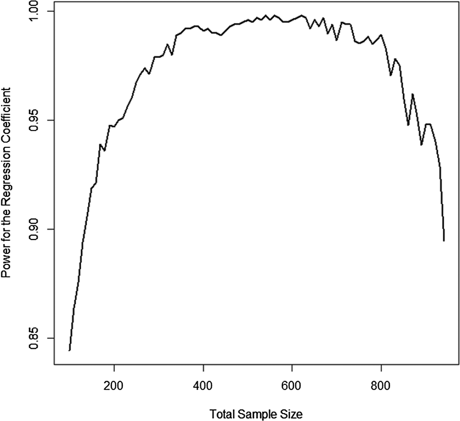
Power for two-method planned missing design.

Conclusions

Planned missing data designs are a powerful tool for minimizing participant burden, making data collection easier, and, with a two-method planned missing data design, maximizing power with set costs. Designing a study with planned missing data requires careful thought about the type of planned missing data design that will be used, and how that planned missing data design is implemented. Monte Carlo simulations provide a method to a priori determine how planned missing data designs will affect power or sample size. Monte Carlo power analyses can be easily implemented in both Mplus and simsem with each software package providing different advantages and disadvantages. One advanced method for power analysis provided in simsem is the ability to vary sample size across replications. When sample size varies across replications, power can be determined across many sample sizes quickly, accurately and efficiently. Mplus has the ability to fit a larger range of models than simsem (e.g. multilevel SEM models). However, Mplus currently does not include facilities for randomly varying sample size, or the ability to integrate multiple imputation into Monte Carlo simulations; functionality that is built into simsem. Researchers who are considering implementing a planned missing data design should first conduct a Monte Carlo power analysis to determine how the planned missing data design will affect power and sample size requirements.

Footnotes

*This article accepted during Marcel van Aken’s term as Editor-in-Chief.

Funding

Partial support for this project was provided by grant NSF 1053160 (Wei Wu & Todd D. Little, co-PIs) and by the Center for Research Methods and Data Analysis at the University of Kansas (when Todd D. Little was director; 2009-2013).

Acknowledgment

Any opinions, findings, and conclusions or recommendations expressed in this material are those of the author(s) and do not necessarily reflect the views of the funding agencies.

Notes

References

Baraldi

A. N.

Enders

C. K.

(2010). An introduction to modern missing data analyses. Journal of School Psychology, 48, 5–37.

Boker

Neale

Maes

H. H.

Wilde

Spiegel

Brick

… Fox

(2011). OpenMx: An open source extended structural equation modeling framework. Psychometrika, 76, 306–317.

Davey

Savla

(2009). Estimating statistical power with incomplete data. Organizational Research Methods, 12, 320–346.

Davey

Savla

(2010). Statistical power analysis with missing data: A structural equation modeling approach. New York, NY: Routledge.

Enders

C. K.

(2010). Applied missing data analysis. New York, NY: Guilford.

Gonzalez

Griffin

(2001). Testing parameters in structural equation modeling: Every “one” matters. Psychological Methods, 6, 258–269.

Graham

J. W.

Taylor

B. J.

Olchowski

A. E.

Cumsille

P. E.

(2006). Planned missing data designs in psychological research. Psychological Methods, 11, 323–343.

Harel

Stratton

Aseltine

(2011). Designed missingness to better estimate efficacy of behavioral studies. In National Center for Health Statistics (Ed.), Tenth conference on health survey research methods (pp. 149–154). Hyattsville, MD: National Center for Health Statistics.

Honaker

King

Blackwell

(2011). Amelia II: A program for missing data. Journal of Statistical Software, 45, 1–47. Available from http://www.jstatsoft.org/v45/i07

10.

Jöreskog

K. G.

(1969). A general approach to confirmatory maximum likelihood factor analysis. Psychometrika, 34, 183–202.

11.

Lai

Kelley

(2011). Accuracy in parameter estimation for targeted effects in structural equation modeling: Sample size planning for narrow confidence intervals. Psychological Methods, 16, 127–148.

12.

MacCallum

R. C.

Browne

M. W.

Cai

(2006). Testing differences between nested covariance structure models: Power analysis and null hypotheses. Psychological Methods, 11, 19–35.

13.

MacCallum

R. C.

Browne

M. W.

Sugawara

H. M.

(1996). Power analysis and determination of sample size for covariance structure modeling. Psychological Methods, 1, 130–149.

14.

Muenchen

R. A.

(2009). R for SAS and SPSS Users. Springer Series in Statistics and Computing. New York, NY: Springer.

15.

Muthén

L. K.

Muthén

B. O.

(2002). How to use a Monte Carlo study to decide on sample size and determine power. Structural Equation Modeling, 4, 599–620.

16.

Muthén

L. K.

Muthén

B. O.

(1998–2013). Mplus user’s guide (7th ed.). Los Angeles, CA: Muthén & Muthén.

17.

Pornprasertmanit

Miller

Schoemann

A. M.

(2013). simsem: SIMulated structural equation modeling (version 0.5-3) [R package]. Available from http://simsem.org/

18.

R Core Team. (2013). R: A language and environment for statistical computing. R Foundation for Statistical Computing, Vienna, Austria. Available from http://www.R-project.org/

19.

Raghunathan

Grizzle

(1995). A split questionnaire survey design. Journal of the American Statistical Association, 90, 54–63.

20.

Rhemtulla

Little

T. D.

(2012). Tools of the trade: Planned missing data designs for research in cognitive development. Journal of Cognition and Development, 13, 425–438.

21.

Rosseel

(2012). lavaan: An R package for structural equation modeling. Journal of Statistical Software, 48, 1–36. Available from http://lavaan.ugent.be/

22.

Satorra

Saris

W. E.

(1985). Power of the likelihood ratio test in covariance structure analysis. Psychometrika, 50, 83–90.

23.

van Buuren

Groothuis-Oudshoorn

, (2011). mice: Multivariate imputation by chained equations in R. Journal of Statistical Software, 45, 1–67.

24.

Verzani

(2004). Using R for Introductory Statistics. London, UK: Chapman and Hall.

Supplementary Material

Please find the following supplemental material available below.

For Open Access articles published under a Creative Commons License, all supplemental material carries the same license as the article it is associated with.

For non-Open Access articles published, all supplemental material carries a non-exclusive license, and permission requests for re-use of supplemental material or any part of supplemental material shall be sent directly to the copyright owner as specified in the copyright notice associated with the article.

0.00 MB

0.03 MB

LY
.7*	0
.7*	0
.7*	0
.7*	0
.7*	0
.7*	0
.7*	0
.7*	0
.7*	0
0	.7*
0	.7*
0	.7*
0	.7*
0	.7*
0	.7*
0	.7*
0	.7*
0	.7*
PS
1	.2*
.2*	1

LY
.7*	0
.7*	0
.7*	0
.7*	0
.7*	0
.7*	0
.7*	0
.7*	0
.7*	0
0	.7*
0	.7*
0	.7*
0	.7*
0	.7*
0	.7*
0	.7*
0	.7*
0	.7*
PS
1	.2*
.2*	1

LY
.7*	0
.7*	0
.7*	0
.7*	0
.7*	0
.7*	0
.7*	0
.7*	0
.7*	0
0	.7*
0	.7*
0	.7*
0	.7*
0	.7*
0	.7*
0	.7*
0	.7*
0	.7*
PS
1	.2*
.2*	1