On the benefits of latent variable modeling for norming scales

Abstract

Structural equation modeling (SEM) is a powerful and flexible analytic tool to model latent constructs and their relations with observed variables and other constructs. SEM applications offer advantages over classical models in dealing with statistical assumptions and in adjusting for measurement error. So far, however, SEM has not been fully used to develop norms of assessments in educational or psychological fields. In this article, we highlighted the norming process of the Supports Intensity Scale – Children’s Version (SIS-C) within the SEM framework, using a recently developed method of identification (i.e., effects-coding method) that estimates latent means and variances in the metric of the observed indicators. The SIS-C norming process involved (a) creating parcels, (b) estimating latent means and standard deviations, (c) computing T scores using obtained latent means and standard deviations, and (d) reporting percentile ranks.

Keywords

effects-coding method of identification norming structural equation modeling supports intensity scale – children’s version

Norming a scale facilitates the interpretation of test results because an individual’s score is referenced against the performance of a standardization sample. Norms are used to identify a person’s strengths and limitations in planning for appropriate services and to monitor personal changes over time or across settings. The Wechsler Intelligence Scale for Children – Fifth Edition (WISC-V; Wechsler, 2014), for example, provides full scale intelligence quotient that represents a student’s cognitive ability based on the norms generated from the standardized sample. The WISC-V also produces the primary index scores (i.e., verbal comprehension, visual spatial, fluid reasoning, working memory, and processing speed) to determine a student’s relative strengths and weaknesses in cognitive processing areas. In describing recommended standardization procedures and guidelines, Cicchetti (1994) emphasized that the standardization of any assessment should systematically stratify the sample on relevant demographic variables. As such, a number of previous studies have established norms in proximal normative reference groups categorized by age, gender, level of education, or ethnicity (e.g., Diehr, Heaton, Miller, & Grant, 1998; Tombaugh, 2004). Researchers can choose among several norming techniques (e.g., linear transformations that preserve or transform the original shape of the raw score distribution, item response theory-based true scores); however, the majority of applied scale development in disability research has tended to use classical test theoretic (CTT) models during the norming process, relying on the means and standard deviations of the observed test scores to compute standard scores (e.g., Powell, MacKrain, & LeBuffe, 2007). In the following section, we (a) compare the CTT models and SEM applications highlighting the strengths of SEM approaches and (b) introduce a norming process that used SEM, which can serve as a guideline for future norming studies.

Comparisons between CTT models and SEM applications

A popular CTT model used for norming is analysis of variance (ANOVA) to examine the mean differences between subgroups (e.g., score differences among age or ethnicity groups, etc.); however, the validity of such norms rests on certain restrictive assumptions of ANOVA that can be easily violated in the applied social and behavioral sciences. The most problematic issue of these assumptions comes hand-in-glove with ANOVA’s use of CTT-based scale scores as dependent variables. In the CTT tradition, scale items are assumed to be measured without error, items are assumed to be interchangeable and equally strong indicators of the unobserved true score (i.e., tau equivalent), and within group variances of the true scores are assumed to be equal (McDonald, 1999). Each of these easily violated assumptions is necessary to ensure the validity of scale scores constructed as simple aggregates (i.e., sums or means) of the observed scores. These assumptions are either unnecessary or easily corrected for with the SEM-based procedure that we propose in what follows.

Methodological experts have advocated using structural equation modeling (SEM) to estimate latent parameters due to the extreme flexibility of the SEM paradigm and the ability to relaxed the assumptions of error-free measurement that plague CTT modeling techniques. SEM is a preferred analytic method because its assumptions are usually more tenable than those of CTT methods, and violations of many of these assumptions are readily correctable (Little, 2013). For example, the multiple-group SEM can easily accommodate heterogeneous population variances by allowing dis-attenuated variances to be estimated in each group and independently corrected to ensure parallel scaling, if necessary, thereby relaxing one of ANOVA’s most limiting assumptions (Fan & Hancock, 2012; Green & Thompson, 2006). Within the SEM framework, between-group differences are most easily tested by nested model chi-squared difference tests, and any such mean comparisons are not influenced by whether the variances are the same or not, whereas heterogeneous variances can severely bias the t tests and F ratios that are usually employed to test for between-group differences in most CTT models. Furthermore, unlike ANOVA, which naively assumes that all observed scores reflect the same level of the latent construct, the SEM approach allows for congeneric indicators. In other words, when using SEM, the degree to which the observed items are associated with the latent variable can vary freely, and, therefore, each item can contribute a different degree of variance to the true score. This is an important strength of the SEM approach for norming. Unlike CTT scores, latent variables fully extract the true score variance from each indicator.

While the most common implementations of both SEM and ANOVA require assuming population-level normality of the observed scores and independent errors, the additional flexibility of the SEM paradigm makes it easier to adjust the fundamental model when these assumptions are violated. For example, most SEM software allows robust estimation methods that yield unbiased parameter estimates and hypothesis tests for non-normal data. Although SEM is no more robust than ANOVA to dependent observations caused by nested data, it can easily accommodate certain type of residual dependence that ANOVA cannot address such as residual covariation between the specific factors of items associated with different constructs.

One of the most critical advantages of SEM is its ability to automatically correct for measurement error when extracting the latent variables. CTT models can only partition the observed scores’ variance into two components: true scores that reflect the proportion of each items variance that is shared with all other items and a single error term that represents all variance not shared with the other items. By incorporating a single error component, CTT models assume that the variables are completely free from measurement error. CTT approaches thereby yield misleading estimates because observed scores are not completely reliable and, often, item residuals are conditionally dependent. Although CTT-based scores can be corrected for measurement error, such corrections must be applied as an additional post-hoc step whereas SEM automatically removes measurement error during model estimation. The assumption of error-free measurement is rarely met in the social and behavioral sciences as nearly all measures have some degree of measurement error and often have correlated residuals. In the SEM framework, the error term is further refined into an item-specific factor that represents the reliable variance that is uniquely associated with each observed indicator and a random error term. Extracting specific factors for each item allows researchers to model possible residual covariation that remains after extracting the true score (e.g., by estimating methods factors). Such informative models of the residual error structure are not possible with CTT approaches. Unlike CTT approaches, the SEM framework uses latent variables to represent true scores that adjust for such measurement issues and produce more trustworthy parameter estimates. Specifically in the norming process, the means and variances, which are corrected for attenuation and other potential measurement problems, lead to more reliable standard scores that represent the accurate relative standings of performance of a person.

Furthermore, the process of extracting latent constructs in the SEM approach actually represents a form of model-based smoothing. In the CTT approach, undesired roughness in the raw score distribution is often pre-smoothed (e.g., using polynomial log-linear method or strong true score method) to remove noise in the observed items or post-smoothed (e.g., using cubic smoothing splines) to remove noise in the distribution of the scale score to improve equating accuracy (Kolen & Brennan, 2014). The process of latent variable modeling, however, maps a set of, possibly, noisy items onto a latent variable that follows a convenient probability distribution. This distribution is often taken to be multivariate normal (as in the application we discuss in what follows), but it can also be a categorical distribution (as in mixture modeling applications) or a non-normal continuous distribution. Because the distribution of the latent variable must be chosen by the researcher to facilitate model estimation, the inherent smoothing of SEM is automatic and absolute. The only roughness in the model-implied distribution of the latent true score comes from having too few observations to accurately represent the probability function. A series of kernel density plots illustrating the smoothing effect of SEM for the SIS-C data are available as online supplementary material at http://www.statscamp.org/sis-c-norming-paper.

Effects-coding method of identification

Although the advantages of SEM applications over CTT models have been continuously addressed in the literature, SEM has not been exploited in the norming process largely because of the problems caused by arbitrary scaling. The traditional scale setting methods of SEM (i.e., fixed factor method and marker variable method) identify mean and covariance parameters in an arbitrary way (Little, Slegers, & Card, 2006). When estimating latent means of constructs in the SEM framework (i.e., multi-group confirmatory factor analysis, subsequently described), the fixed factor method fixes the variances and the means of the latent constructs to be one and zero, respectively, in the first group, and allows latent variances and latent means in subsequent groups to be freely estimated. In this way, the estimates of the means and variances of latent constructs are determined in relation to the fixed mean and variance in the initial group. The marker variable method also provides arbitrary scaling by fixing the intercept and factor loading of one of the indicators in each construct to zero and one, respectively. The means and variances of latent constructs are estimated in all groups, but these estimates are all scaled relative to the marker variable chosen for identification. The fixed factor and marker variable methods (the two traditional scaling methods) are not appropriate for deriving norms because they produce estimates that are in an arbitrary metric and cannot be conveniently used to create standard scores during the norming process.

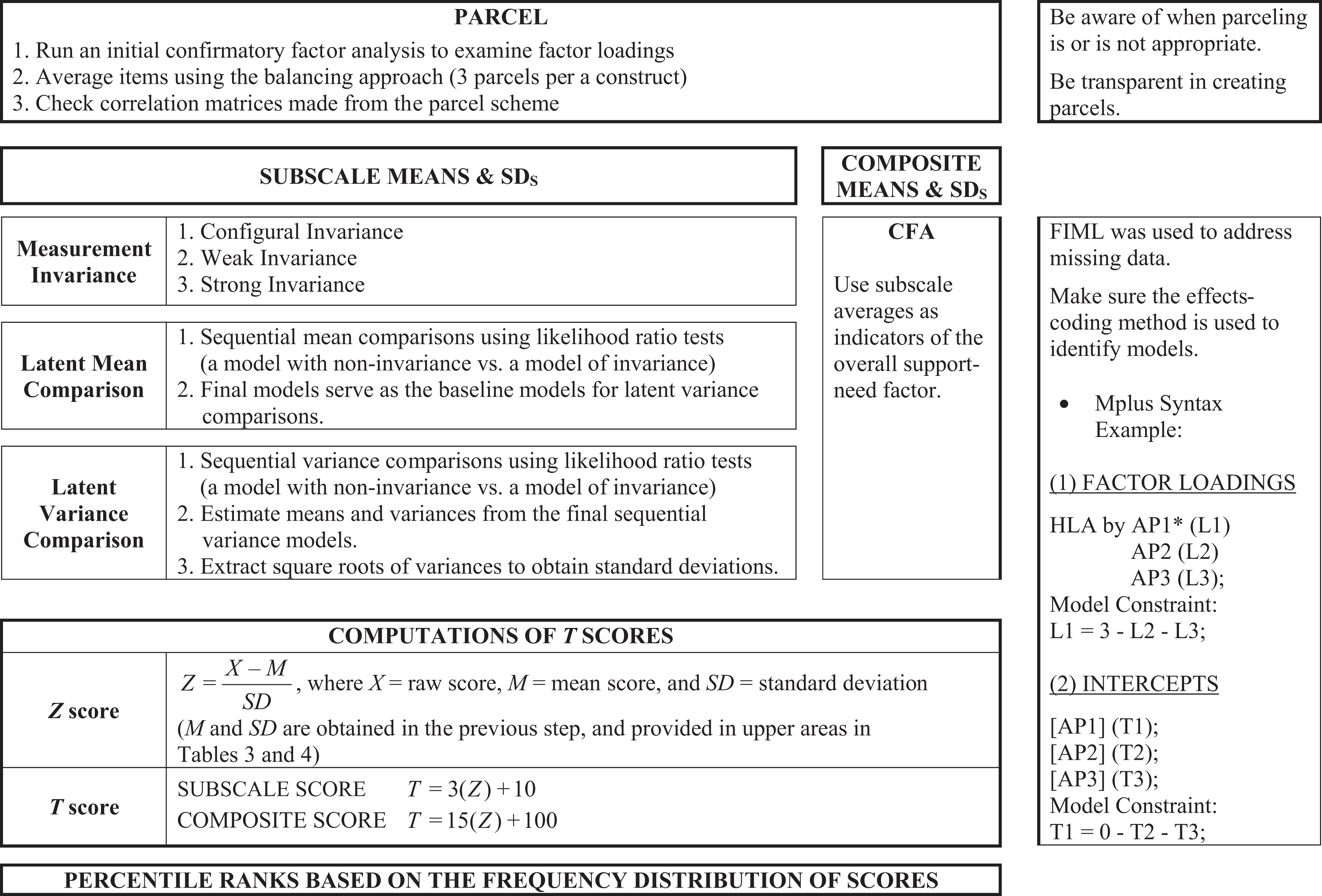
Little et al. (2006) introduced the effects-coding method of identification, which maintains the metric of the original scale of the observed indicators and is, therefore, non-arbitrary. The effects-coding method of identification is accomplished by placing specific constraints so that the factor loadings of a given construct all average to one, and while the average of each constructs intercepts is constrained to zero (sample Mplus syntax is provided in Figure 1). The effects-coding method of identification generates the same model fit and estimates of latent effect sizes as the traditional scaling methods. However, the meaningful scaling metric obtained from the effects-coding method is preferable when the study focus is to “test whether the mean or variance of one latent variable is different from the mean or variance of another latent variable within either single- or multiple-group models” (Little et al., 2006, p. 68) because it leads to differences given in units of the original scales rather than on an arbitrary metric. This advanced feature of effects-coding scaling enables confirmatory factor analysis models to become a tool for norming scales. Because effects-coding produces a metric that is based on the average of the indicators, all norms are therefore constructed as the average, rather than the sum, of the indicators of a given construct.

Figure 1.

An overview of SIS-C norming process (the total number of norming sample = 4,015).

Purpose of the study

The purpose of this study is to introduce a series of SEM applications that use the effects-coding method of identification, so that researchers can use the latent variable modeling to develop norms when the type of measurement is not ordinal. To do this, this study provides an example that used the SEM technique to norm the Supports Intensity Scale – Children’s Version (SIS-C), a measure of the intensity of support needs developed for children and youth with intellectual disability. In the following section, we address a brief description of the SIS-C, review the norming process in the SEM framework (see Figure 1), and highlight the benefits of SEM applications to create standard scores (i.e., T scores and percentile ranks).

The case study (SIS-C)

Support needs is defined as the “pattern and intensity of supports necessary for a person to participate in activities linked with normative human functioning” (Thompson et al., 2009, p. 135). The first tool developed to measure support needs in adults with intellectual disability was the Supports Intensity Scale – Adult Version (SIS-A, Thompson et al., 2004; Thompson, Bryant et al., 2015). It was normed on a sample of 1,306 people between the ages of 16 and 64 years with intellectual disability. There was also a need for standardized assessments to measure support needs of children and youth with intellectual disability aged 5 to 16 years, leading to the development of the Supports Intensity Scale – Children’s Version (SIS-C, Thompson, Wehmeyer, et al., in press). The norming procedures that are being undertaken to standardize the SIS-C are presented in this article as a case study. The SIS-A was normed using CTT models, whereas the SEM approach was used to norm the SIS-C. The next section describes the norming process of the SIS-C.

Sampling

The normative sample consisted of 4,015 children and adolescents between ages of 5 and 16 with intellectual disability. Data were collected from either state Developmental Disabilities systems (n = 2,910; 72.5% of cases) or school districts (n = 1,105; 27.5% of cases) in 23 states, representing all geographic areas of the United States. Males constituted 67.5% (n = 2,710) of the total sample, whereas females made up 29.9% (n = 1,202). There were 103 participants who did not indicate their gender (n = 103, 2.6%). Table 1 provides additional information on demographic characteristics of children/adolescents who were rated.

Table 1.

Demographic characteristics of normative sample.

Variable	n (imputed n)	%
Data source
State developmental disabilities systems	2,910	72.5
School districts	1,105	27.5
Gender
Male	2,710	67.5
Female	1,202	29.9
Missing	103	2.6
Age cohort
5–6	513 (513)	12.8
7–8	562 (562)	14.0
9–10	762 (787)	19.0
11–12	804 (844)	20.0
13–14	818 (822)	20.4
15–16	487 (487)	12.1
Missing	69	1.7
Ethnicity
White	2,244	55.9
Black	820	20.4
Hispanic	384	9.6
Multiple ethnic backgrounds	237	5.9
Asian/Pacific Islander	159	4.0
Native American	26	0.6
Other	73	1.8
Missing	72	1.8
Student’s intelligence level
< 25 or profound	459	11.4
25–39 or severe	862	21.5
40–55 or moderate	1,321	32.9
55–70 or mild	1,157	28.8
Missing	216	5.4
Student’s adaptive behavior level
Profound	563	14.0
Severe	1,052	26.2
Moderate	1,335	33.3
Mild	948	23.6
Missing	117	2.9

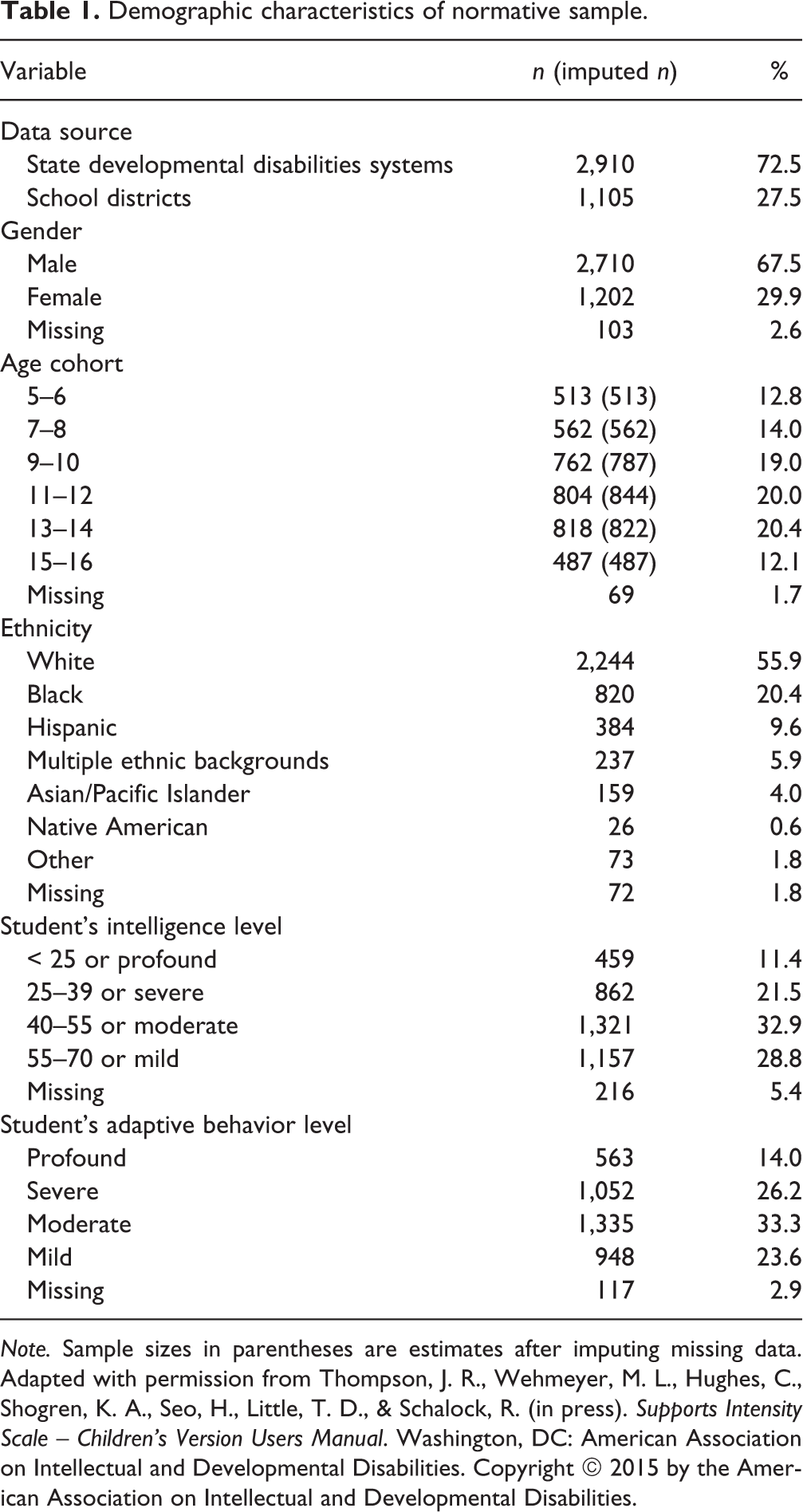
Note. Sample sizes in parentheses are estimates after imputing missing data. Adapted with permission from Thompson, J. R., Wehmeyer, M. L., Hughes, C., Shogren, K. A., Seo, H., Little, T. D., & Schalock, R. (in press). Supports Intensity Scale – Children’s Version Users Manual. Washington, DC: American Association on Intellectual and Developmental Disabilities. Copyright © 2015 by the American Association on Intellectual and Developmental Disabilities.

As previously mentioned, norming needs to be conducted with systematic stratification on the relevant demographic variables. As children experience substantial changes within the span of a year or two, the SIS-C Task Force decided to stratify six age groups that varied by 2 years: 5–6-year-olds, 7–8-year-olds, 9–10-year-olds, 11–12-year-olds, 13–14-year-olds, and 15–16-year-olds. Given these strata, norms and standard scores (seven subscale standard scores, a composite standard score, and corresponding percentile ranks) were developed for each age band. As seen in Table 1, 69 cases (1.7% of the sample) did not have age information. These missing data were imputed 100 times with the R (R Development Core Team, 2008) package Amelia II (Honaker, King, & Blackwell, 2011) using all SIS-C items as predictors in the imputation model. Final estimates for each missing age value were computed as the averages of 100 imputed age replicates. It should be noted that multiple imputation is designed to facilitate estimation of population parameters and not to correctly replicate the missing data points. In this study, the person-level ages can be viewed as the parameters to estimate. The multiple imputation procedure resulted in 100 draws from each participant’s posterior predictive distribution of age, and, by averaging these 100 draws (i.e., taking the mean of the 100 imputed age variables), we have assigned each participant their most likely age value. Therefore, our implementation still follows sound missing data theoretic principles. Although age was not normally distributed in this sample, semi-parametric imputation methods (i.e., predictive mean matching) produced unreasonable imputations of the 69 missing ages (i.e., imputing a constant value of five for all missing ages) and convergence failures precluded imputation of the categorized age variable via generalized linear models explicitly designed for ordinal variables. Running the following analyses without the 69 observations missing age did not change any of the results. Specifically, two latent means of Home Life (11–12 and 13–14-year-olds) and five latent means of School Participation (5–6, 7–8, 9–10, 11–12, and 13–14-year-olds) were different; however, all differences were found at three decimal places. The detailed results from this sensitivity analysis are available at http://www.statscamp.org/sis-c-norming-paper. After using a best-practice missing data treatment (see below), there were 669 children/youth, on average, in each cell. Estimates in parentheses in Table 1 represent imputed sample sizes for the age bands.

Measure

The SIS-C consists of two main sections: (a) exceptional medical and behavioral needs and (b) Supports Needs Index Scale. The first section of exceptional medical and behavioral needs measure medical conditions and challenging behaviors that would influence support needs of children and youth with intellectual disability. Exceptional medical and behavioral support needs are rated by a scale of 0 to 2; these ratings are not included in the standard scores. The second section of the SIS-C consists of seven life activities: Home Life, Community and Neighborhood, School Participation, School Learning, Health and Safety, Social, and Advocacy. Scores from these seven subscales are used to calculate the composite standard score, a SIS Support Needs Index, to present an indication of the intensity of a person’s support needs with respect to the peer normative sample. Each item on these seven subscales is rated by three dimensions on a 0–4 Likert scale: frequency, daily support time, and type of support. The average scores across these three dimensions were included in the SEM models to maintain identical scales of metrics for each construct being measured.

Norming step

Figure 1 provides an overview that summarizes each norming step involved in the SIS-C; (a) parcel as a pre-modeling step, (b) estimate latent means and standard deviations of constructs, (c) calculate T scores using latent means and standard deviations obtained in the previous step, and (d) find percentile ranks based on the frequency distribution of the scores. Details on each step are addressed in the following section; steps (b), (c), and (d) include comparisons of parameter estimates obtained from latent and manifest spaces to present the advantages of SEM applications over CTT models.

Step one: parcel

The primary goal of the SEM application in the norming process is to obtain reliable latent means and standard deviations of constructs. As our intent is to understand the nature of the latent constructs, and not the item-level relationships, we created parcels of the observed items to act as indicators of each construct (Little, Rhemtulla, Gibson, & Schoemann, 2013). Parcels, a meaningful set of items that convey manifest information into the latent space, reduce the specific variances of each item (i.e., increase the proportion of true-score variance leading to higher reliability and greater communality). This feature of parcels enhances the psychometric properties of the data, but parceling can also facilitate model estimation with high-dimensional data. Models with parcels have fewer parameter estimates and more parsimonious representations of the latent constructs than original indicators. The aforementioned feature of parcels is particularly beneficial in our study as stratifying on age led to a very large model (i.e., a seven-construct CFA model with a total of 61 items, and this CFA model was replicated in six age bands). Without parcels, this model had considerable problems with convergence and unstable parameter estimates. Parcels were created by examining the item-level information and averaging the items in a way that reduces nuisance variance with no loss of generality regarding inferences about the latent construct (Little, Rhemtulla, et al., 2013). It should be noted, however, that parcels are not recommended when the focus of study is the behavior of the items themselves, especially during the exploratory stage of scale development. The use of parcels is only warranted when researchers examine the relations among latent constructs based on items with properties and behaviors that are already well-established.

Parcels should be created with careful consideration based on both theoretical and empirical guidance (Little, Rhemtulla, et al., 2013). To create the parcels for this study, we first ran an item-level confirmatory factor analysis (CFA) using the total sample (n = 4,015) to identify the behavior of items and their relations. Next, based on factor loadings obtained from the CFA, the balancing approach was used to create parcels by “assign[ing] the item with the highest item-scale correlations to be paired with the item that has the lowest item-scale correlation” (Little, 2013, p. 24) and computing the row-wise averages of the selected items to construct each parceled indicator. The balancing approach enabled us to find the location of a construct’s centroid by generating a set of essentially tau-equivalent indicators (i.e., indicators with approximately equal strengths of association to the construct). Based on Little’s (2013) suggestion, we created three parcels per each construct so that each construct can be precisely defined by a just-identified measurement structure. For a detailed discussion of parcel construction and an illustration of the balancing technique, in particular, see Little (2013, Chapter 1). Astute readers may have noticed that there was a small amount of missing data on the SIS-C items (i.e., < 0.7%) which we averaged over when creating the parcels. This practice (i.e., averaging available items) is not generally advisable. When creating parcels from incomplete data, we generally recommend imputing the item-level missingness before parcel creation. For the current study, however, imputing the item level missingness and averaging the available items produced equivalent results due to the trivially low nonresponse rate (with nonresponse rates < 1%, the missing data treatment will have minimal impact on the analysis outcomes; Little, Jorgenson, Lang, & Moore, 2013). Three standard deviations of school participation domain (9–10, 11–12, and 13–14-year-olds) were different at three decimal places when comparing results from two approaches (imputing the item level missingness vs. averaging the available items). The complete results from this sensitivity analysis are provided at http://www.statscamp.org/sis-c-norming-paper.

In order to create a universal parceling structure that functions equally well across all age groups, we made modifications to this initial parceling scheme, when testing for configural invariance, in order to ensure factorial comparability across all age groups. Table 2 provides the parcel scheme that was optimal across the age bands; the corresponding correlation matrices are provided in the Appendix (note that several correlations within the same construct have weak relations due to inherent sampling errors around the true population values). This final parcel structure was used in the entire norming process of the SIS-C. Information on the raw score distribution and the parceled score distribution (i.e., mean, standard deviation, skewness, and kurtosis) is available as online supplementary material at http://www.statscamp.org/sis-c-norming-paper.

Table 2.

Parcel schemes for each construct.

Construct	Parcel	Item
Home life activities	AP1	5. Using the toilet
		8. Keeping self-occupied during unstructured time (free time) at home
		9. Operating electronic devices
	AP2	2. Eating
		3. Washing and keeping self-clean
		6. Sleeping and/or napping
	AP3	1. Completing household chores
		4. Dressing
		7. Keeping track of personal belongings at home
Community & neighborhood activities	BP1	1. Moving around the neighborhood and community
		4. Using public services in one’s community or neighborhood
		7. Complying with basic community standards, rules, and/or laws
	BP2	3. Participating in leisure activities that do not require physical exertion.
		6. Shopping
		8. Attending special events in the community or neighborhood such as cookouts/picnics, cultural festivals, music/art fairs, or holiday oriented events
	BP3	2. Participating in leisure activities that require physical activity
		5. Participating in community service and religious activities
School participation activities	CP1	1. Being included in general education classrooms
		2. Participating in activities in common school areas (e.g., playground, hallways, cafeteria)
		3. Participation in co-curricular activities
	CP2	4. Getting to school (includes transportation)
		5. Moving around within the school and transitioning between activities
		9. Keeping track of schedule at school
	CP3	6. Participating in large-scale test taking activities required by state education systems
		7. Following classroom and school rules
		8. Keeping track of personal belongings at school
School learning activities	DP1	2. Learning academic skills
		3. Learning and using metacognitive strategies
		5. Learning how to use and using educational materials, technologies, and tools
		6. Learning how to use and using problem solving and self-regulation strategies in the classroom
	DP2	4. Completing academic tasks (e.g., time, quality, neatness, organizational skills)
		9. Completing homework assignments
	DP3	1. Accessing grade level curriculum content
		7. Participating in classroom level evaluations, such as tests
		8. Accessing the health and physical education curricula
Health & safety activities	EP1	3. Maintaining emotional well-being
		5. Implementing routine first aid when experiencing minor injuries such as a bloody nose
		8. Avoiding health and safety hazards
	EP2	1. Communicating health related issues and medical problems, including aches and pains
		2. Maintaining physical fitness
		7. Protecting self from physical, verbal, and/or sexual abuse
	EP3	4. Maintaining health and wellness 6. Responding in emergency situations
Social activities	FP1	2. Respecting the rights of others
		4. Responding to and providing constructive criticism 7. Communicating with others in social situations
	FP2	3. Maintaining conversation
		5. Coping with changes in routines and/or transitions across social situations
		8. Respecting others personal space/property
	FP3	1. Maintaining positive relationships with others
		6. Making and keeping friends
		9. Protecting self from exploitation and bullying
Advocacy activities	GP1	3. Taking action and attaining goals
		5. Advocating for and assisting others
		7. Communicating personal wants and needs
	GP2	1. Expressing preferences
		2. Setting personal goals
		6. Learning and using self-advocacy skills
	GP3	4. Making choices and decisions
		8. Participating in educational decision making
		9. Learning and using problem solving and self-regulation strategies in the home and community

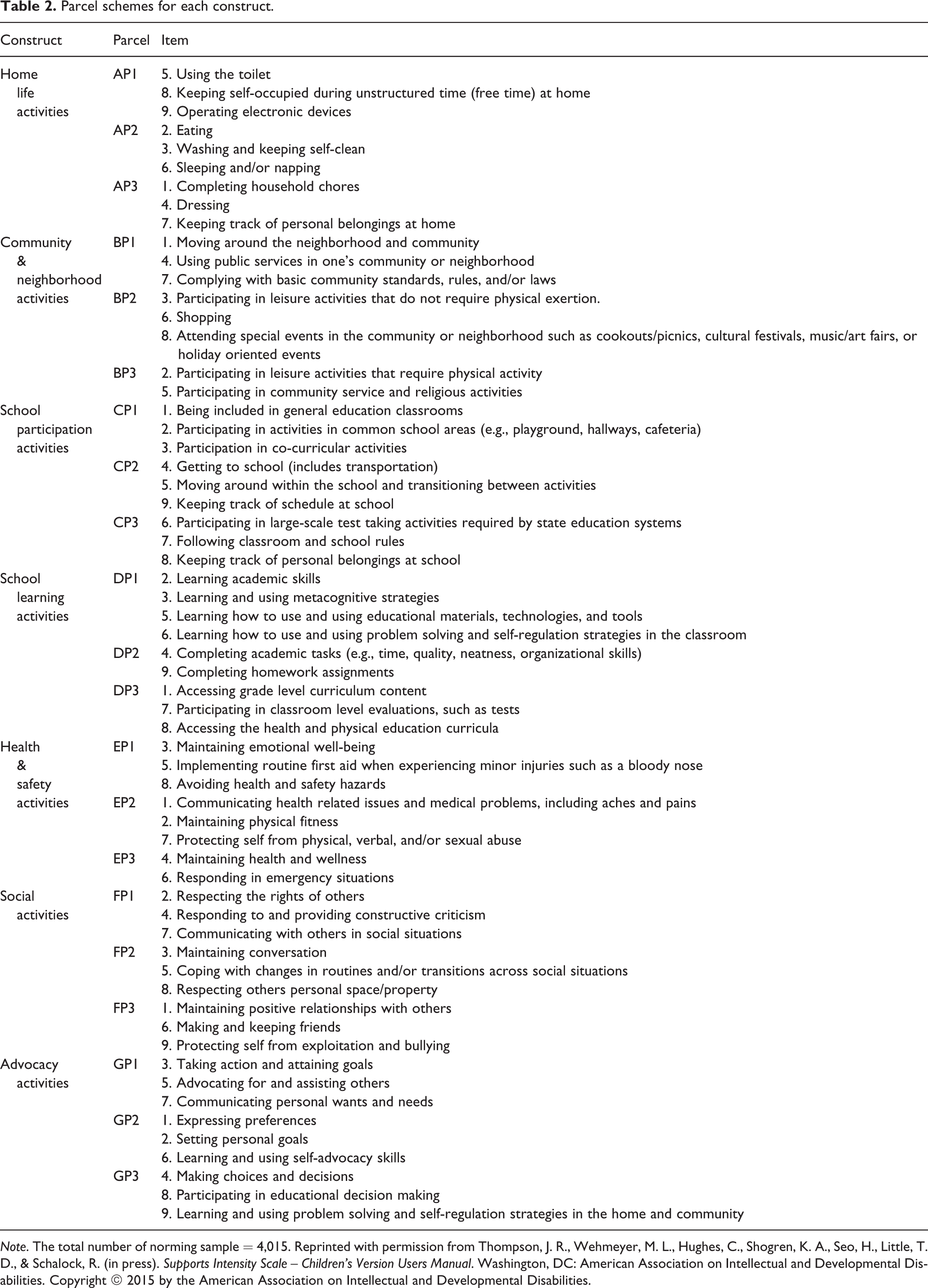
Note. The total number of norming sample = 4,015. Reprinted with permission from Thompson, J. R., Wehmeyer, M. L., Hughes, C., Shogren, K. A., Seo, H., Little, T. D., & Schalock, R. (in press). Supports Intensity Scale – Children’s Version Users Manual. Washington, DC: American Association on Intellectual and Developmental Disabilities. Copyright © 2015 by the American Association on Intellectual and Developmental Disabilities.

Step two: estimate latent means and standard deviations

Multiple-group Mean and Covariance Structures (MACS; Little, 1997) CFA was performed to establish measurement equivalence of the SIS-C across six age bands as well as to estimate latent means and standard deviations of constructs. Mplus version 7.0 (Muthén & Muthén, 2012) was used for the following data analyses. As emphasized in the introduction section, the effects-coding method of identification was used to obtain all latent means and variances. The example syntax for effects-coding method of identification is provided in Figure 1. The complete Mplus syntax for MACS CFA is available as online supplementary material at http://www.statscamp.org/sis-c-norming-paper.

Multiple-group confirmatory factor analysis

The multiple-group CFA is performed by two sets of evaluation: tests of measurement invariance and tests of the structural parameters (Brown, 2015). First, the measurement invariance—sometimes referred to as construct comparability or measurement equivalence— is examined by sequential tests at three invariance levels: configural invariance, weak invariance, and strong invariance. The purpose of measurement invariance testing is to establish construct comparability across subgroups (i.e., is the SIS-C measuring each support-need construct equivalently across six age bands?). Thus, measurement invariance tests are simply multivariate tests for differential item functioning (DIF). The test of measurement invariance is an essential step to test the equality of the structural parameters because established measurement equivalence eliminates potential confounding effects of the grouping variable that can impact differences in latent means and variances (Little, 2013). In other words, by confirming equivalent measurement properties in the subgroups of the population, a concern about “test bias” involved in scales can be alleviated before obtaining standard scores (Brown, 2015, p. 3), and this feature is one of the key strengths of SEM applications in norming scales.

Next, after establishing measurement invariance, structural parameters are evaluated to test differences in latent parameters (latent means, latent variances) of the SIS-C across six subgroups. To derive the means used to compute norms within each age group, a series of models were tested. An omnibus latent mean comparison was initially performed by imposing seven sets of invariance constraints on construct means across age groups in the strong invariance model. Additional tests were subsequently employed to detect which latent constructs had mean differences across groups and to further find the age groups that differed from each other on a given construct. To estimate latent means in each age group, sequential mean comparisons were conducted by evaluating the impact of adding equality constraints on factor means across age groups. For example, we initially equated the Advocacy latent means between 5–6 and 7–8 age groups. When the Advocacy latent means between these two age groups were not statistically different based on the Bonferroni correction (i.e., alpha level .01/ the total number of comparisons), we additionally imposed an equality constraint on the Advocacy of the 9–10 age group to make the Advocacy means of 5–6, 7–8, and 9–10 age groups equated. Then we conducted the likelihood test (i.e., model with equality constraints on 5–6 and 7–8 age groups vs. model with equality constraints on 5–6, 7–8, and 9–10 age groups) to examine the impact of an additional equality constraint.

As parallel analyses to test the equivalence of the latent variances and estimate the standard deviations of constructs, seven sets of equality constraints were placed on construct variances across groups in previously identified final sequential mean models. When equality constraints were not tenable, follow-up tests were conducted to determine which constructs had variance differences and to examine specific patterns of variance differences across groups on a given construct. As in the latent mean comparisons, sequential comparisons using the Bonferroni corrections were performed to test similarities and differences in variances and to provide variance estimates across age groups. The constructs’ standard deviations were then estimated by taking square roots of the variances. These standard deviations, along with the latent means estimated from the final sequential models, were used to generate norms.

A comprehensive overview of the empirical results and discussions from the aforementioned multiple-group CFA is beyond the scope of this article. See Shogren et al. (in press) for more information on results from the multiple-group CFA described above. The focus of this study is to introduce the norming procedure within the SEM approach and to present the strengths of SEM applications by comparing norms and subscale standard scores in the latent space with corresponding counterpart estimates at the manifest space. To obtain the latent means and standard deviations needed to calculate composite standard scores for the age groups, we conducted additional confirmatory factor analyses that include subscale averages as parceled indicators of the overall support-need factor. The effects-coding method of identification was again used to obtain non-arbitrary latent estimates that are in the metric of the manifest indicators.

Estimated latent means and standard deviations

Table 3 (upper area) provides latent means (which are also reported and discussed in Shogren et al., in press) and the raw means of the constructs. Here, there are two considerations when comparing latent and manifest estimates. As addressed in the “multiple-group confirmatory factor analysis” section, the latent means are estimated from constrained models. The constrained models provide a better estimate of age-norms than the unconstrained models because sources of sampling variability within each age band are minimized (Little, 2013). Table 3 (bottom area) provides all estimates from the unconstrained models. The CTT-based and SEM-based analyses also used two different missing data approaches: full information maximum likelihood (FIML; a model-based missing data approach) estimation was used for the latent space analyses; pair-wise deletion was used for the manifest space analyses (in this sample, the range of missing data was negligible: 0 to 0.7%). Although utilizing a modern principled missing data tool for the latent variable analyses and an antiquated ad hoc missing data treatment for the CTT analyses may seem like an unfair comparison, it is also an accurate representation of the state of missing data practice. For many years, deletion-based techniques have remained the most common missing data treatment employed in applied studies that utilize CTT models, while FIML is consistently chosen to treat missingness when employing latent variable models (Bodner, 2006; Little, Jorgenson, et al., 2013; Peugh & Enders, 2004). Thus, we have chosen these methods purposefully to optimize external, ecological validity rather than unduly prioritizing internal validity and experimental control. The means obtained from both approaches were highly congruent, but this congruence should certainly not be taken as an endorsement of deletion-based missing data treatments which should not be employed in practice (Little, Jorgenson, et al., 2013).

Table 3.

Means at both latent and raw levels.

Construct	5–6		7–8		9–10		11–12		13–14		15–16
Construct	Latent	Raw	Latent	Raw	Latent	Raw	Latent	Raw	Latent	Raw	Latent	Raw
< Estimates from constrained models >
Home life	2.64	2.64	2.45	2.47	2.45	2.44	2.28	2.31	2.28	2.24	2.03	2.03
Community and neighborhood	2.90	2.98	2.90	2.89	2.90	2.87	2.78	2.79	2.78	2.77	2.60	2.60
School participation	3.01	3.10	3.01	3.07	3.01	3.03	3.01	2.98	3.01	2.94	2.74	2.74
School learning	3.27	3.26	3.27	3.31	3.27	3.30	3.27	3.29	3.27	3.27	3.14	3.15
Health and safety	3.06	3.10	3.06	3.05	3.06	3.01	2.92	2.95	2.92	2.88	2.70	2.69
Social	3.04	3.08	3.04	3.05	3.04	3.00	2.83	2.88	2.83	2.79	2.59	2.59
Advocacy	2.97	3.03	2.97	2.99	2.97	2.98	2.97	2.94	2.97	2.91	2.76	2.76
< Estimates from unconstrained models >
Home life	2.64	2.64	2.47	2.47	2.44	2.44	2.31	2.31	2.24	2.24	2.03	2.03
Community and neighborhood	2.97	2.98	2.88	2.89	2.86	2.87	2.79	2.79	2.77	2.77	2.60	2.60
School participation	3.11	3.10	3.07	3.07	3.03	3.03	2.98	2.98	2.94	2.94	2.74	2.74
School learning	3.25	3.26	3.29	3.31	3.28	3.30	3.28	3.29	3.25	3.27	3.14	3.15
Health and safety	3.11	3.10	3.07	3.05	3.03	3.01	2.95	2.95	2.89	2.88	2.70	2.69
Social	3.09	3.08	3.05	3.05	3.00	3.00	2.87	2.88	2.79	2.79	2.59	2.59
Advocacy	3.04	3.03	3.01	2.99	2.99	2.98	2.94	2.94	2.90	2.91	2.76	2.76
Total	3.03	3.03	2.98	2.98	2.95	2.95	2.88	2.87	2.83	2.83	2.65	2.65

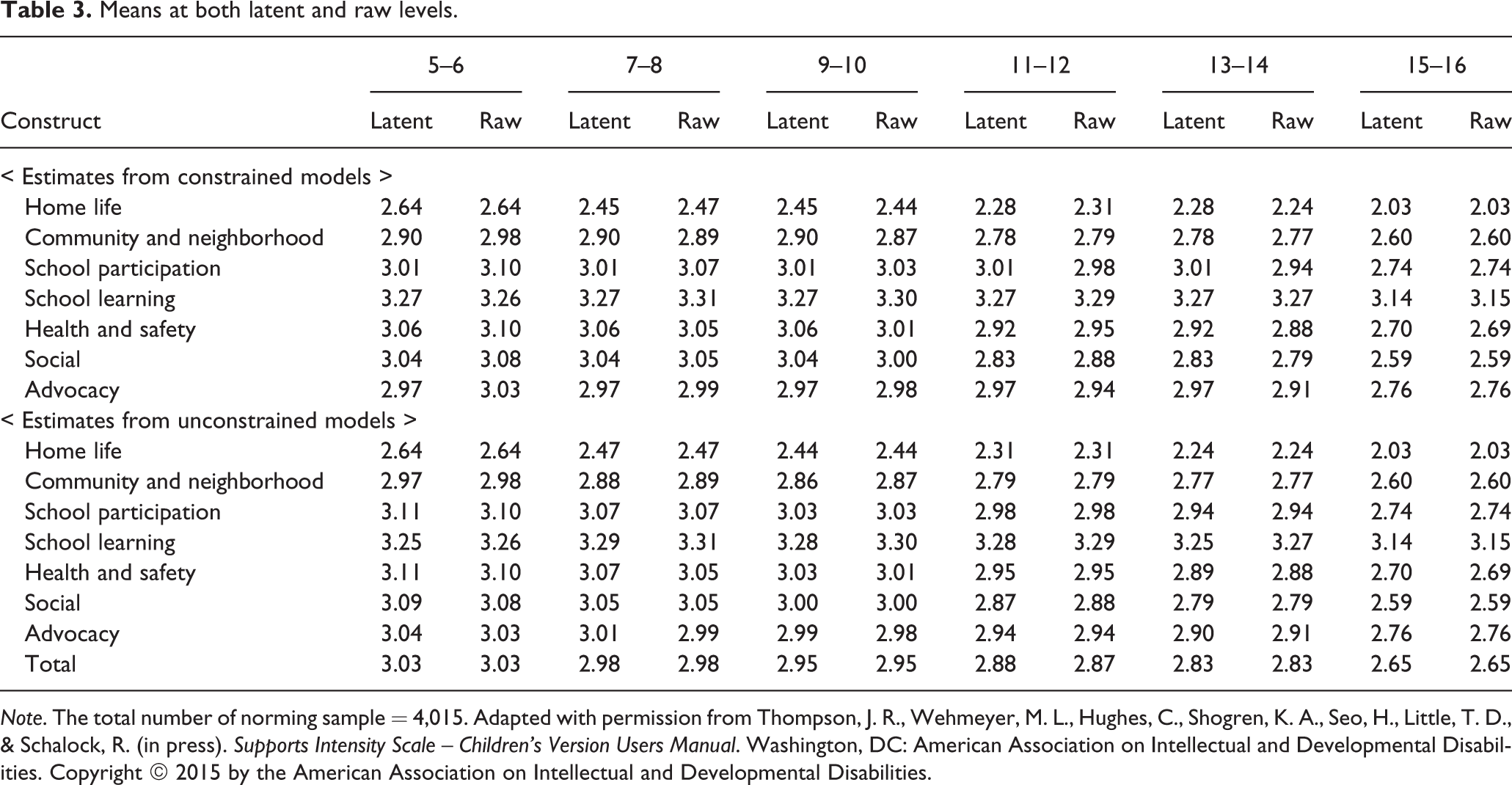
Note. The total number of norming sample = 4,015. Adapted with permission from Thompson, J. R., Wehmeyer, M. L., Hughes, C., Shogren, K. A., Seo, H., Little, T. D., & Schalock, R. (in press). Supports Intensity Scale – Children’s Version Users Manual. Washington, DC: American Association on Intellectual and Developmental Disabilities. Copyright © 2015 by the American Association on Intellectual and Developmental Disabilities.

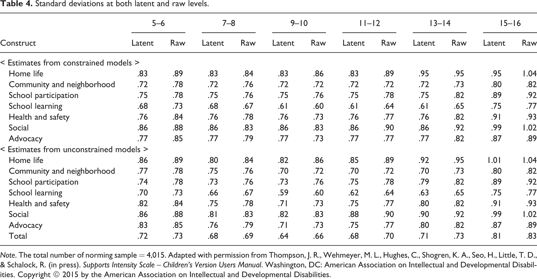
As expected, however, we found pronounced differences between latent and raw standard deviations. The dis-attenuated standard deviations at the latent space provide error-free estimates of variability for calculating standard scores and understanding the relative standing of support needs in the normative sample. The raw score standard deviations contain error variance in the estimates. Similar to the process used for mean comparisons between latent and raw levels, we used latent standard deviations estimated from the constrained models to minimize sampling variability in the norming scores (upper area in Table 4). For comparative purposes, we also report, at the bottom area in Table 4, the estimates from the models that did not have any constraints imposed on the latent variances across groups.

Table 4.

Standard deviations at both latent and raw levels.

Construct	5–6		7–8		9–10		11–12		13–14		15–16
Construct	Latent	Raw	Latent	Raw	Latent	Raw	Latent	Raw	Latent	Raw	Latent	Raw
< Estimates from constrained models >
Home life	.83	.89	.83	.84	.83	.86	.83	.89	.95	.95	.95	1.04
Community and neighborhood	.72	.78	.72	.76	.72	.72	.72	.72	.72	.73	.80	.82
School participation	.75	.78	.75	.76	.75	.76	.75	.78	.75	.82	.89	.92
School learning	.68	.73	.68	.67	.61	.60	.61	.64	.61	.65	.75	.77
Health and safety	.76	.84	.76	.78	.76	.73	.76	.77	.76	.82	.91	.93
Social	.86	.88	.86	.83	.86	.83	.86	.90	.86	.92	.99	1.02
Advocacy	.77	.85	.77	.79	.77	.73	.77	.77	.77	.82	.87	.89
< Estimates from unconstrained models >
Home life	.86	.89	.80	.84	.82	.86	.85	.89	.92	.95	1.01	1.04
Community and neighborhood	.77	.78	.75	.76	.70	.72	.70	.72	.70	.73	.80	.82
School participation	.74	.78	.73	.76	.73	.76	.75	.78	.79	.82	.89	.92
School learning	.70	.73	.66	.67	.59	.60	.62	.64	.63	.65	.75	.77
Health and safety	.82	.84	.75	.78	.71	.73	.75	.77	.80	.82	.91	.93
Social	.86	.88	.81	.83	.82	.83	.88	.90	.90	.92	.99	1.02
Advocacy	.83	.85	.76	.79	.71	.73	.75	.77	.80	.82	.87	.89
Total	.72	.73	.68	.69	.64	.66	.68	.70	.71	.73	.81	.83

Steps three and four: compute standard scores (T score and percentile ranks)

Two types of score transformations are reported for each SIS-C subscale: T score and percentile rank. To obtain T scores as linear transformations of the normal deviate, we first calculated Z scores using the latent means and standard deviations of each SIS-C subscale in a given age group (upper areas in Table 3 and Table 4). The equation provided in Figure 1 was used to compute Z scores. Next, we converted these Z scores to T scores with a mean of 10 and a standard deviation of 3 to maintain a comparable distribution to the SIS-A and other intelligence and adaptive behavior scales (see Thompson, Wehmeyer, et al., in press). Figure 1 provides the equation used to obtain T scores for subscale scores.

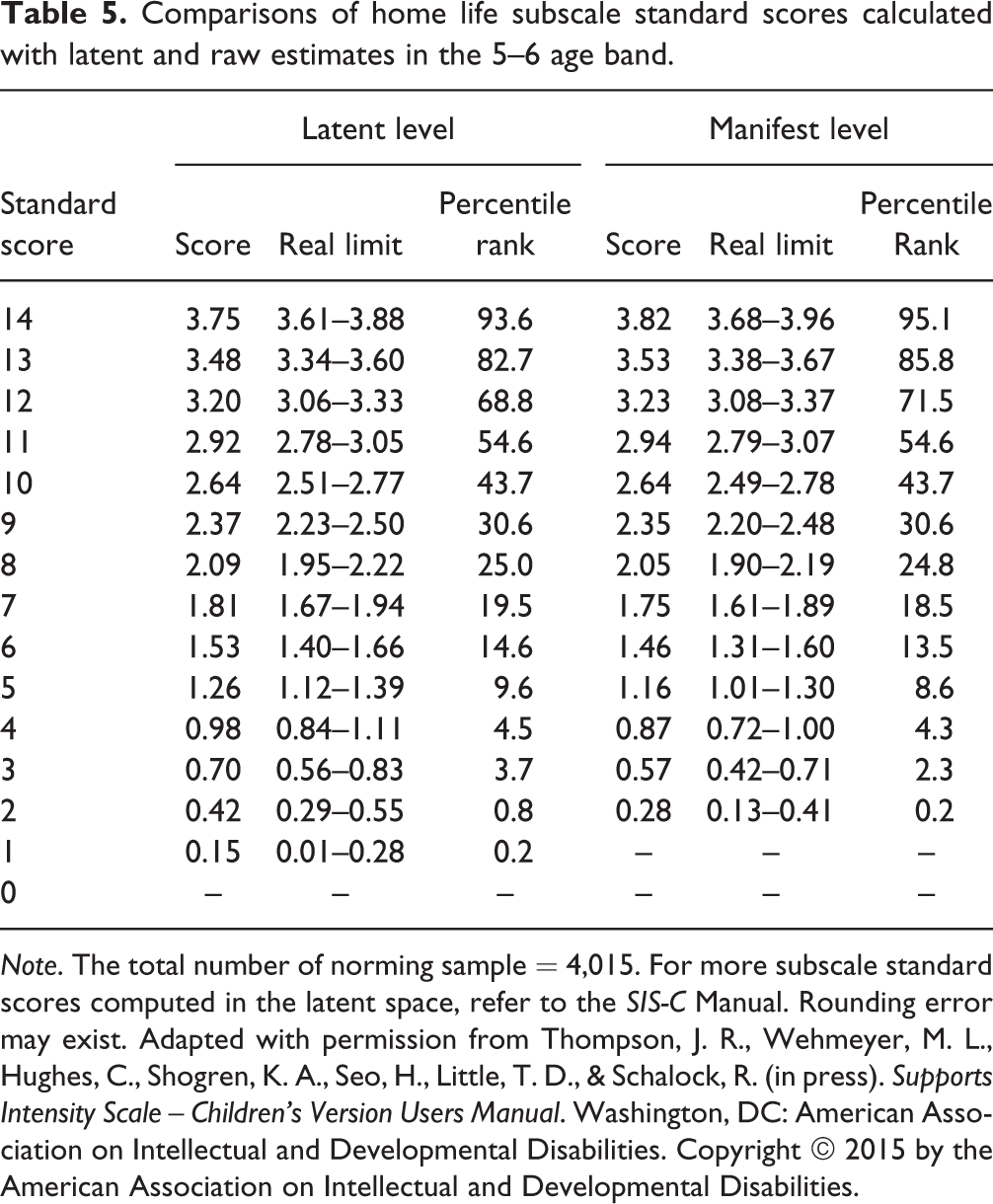
In addition, percentile ranks are reported for each support-need construct in a given age group. Percentile ranks are nonlinear score transformations and serve as auxiliary score scales to improve the interpretation of raw scores on norm-referenced tests (Kolen, 2006). For example, at a certain point in the distribution of scores, a given raw score is greater than or equal to 80% of the scores of the normative sample; this score would be at the 80th percentile rank. Table 5 provides subscale standard scores (T scores), real limits, and percentile ranks of the Home Life domain within the 5–6 age band that are calculated using both latent and manifest means and standard deviations. The real limits of class intervals were provided for the convenience of the SIS-C users; real limits are defined as “the point falling exactly halfway between the two score values, indicating the upper boundary of one interval and the lower boundary of the other interval” (Shavelson, 1996, p. 51). The average score of items leads to different T scores and percentile ranks depending on the approach used. For example, the average score of Home Life domain of 3.75 is converted to a subscale T score of 14 and a percentile rank of 94 in the latent metric, whereas a slightly higher score of 3.82 is converted to the same subscale T score of 14 but with a different percentile rank of 95. In addition, with regard to real limits of class intervals, a person with a 3.61 score would have the subscale T score of 14 at the latent level, whereas the same score leads to the subscale T score of 13 at the manifest level.

Table 5.

Comparisons of home life subscale standard scores calculated with latent and raw estimates in the 5–6 age band.

Standard score	Latent level			Manifest level
Standard score	Score	Real limit	Percentile rank	Score	Real limit	Percentile Rank
14	3.75	3.61–3.88	93.6	3.82	3.68–3.96	95.1
13	3.48	3.34–3.60	82.7	3.53	3.38–3.67	85.8
12	3.20	3.06–3.33	68.8	3.23	3.08–3.37	71.5
11	2.92	2.78–3.05	54.6	2.94	2.79–3.07	54.6
10	2.64	2.51–2.77	43.7	2.64	2.49–2.78	43.7
9	2.37	2.23–2.50	30.6	2.35	2.20–2.48	30.6
8	2.09	1.95–2.22	25.0	2.05	1.90–2.19	24.8
7	1.81	1.67–1.94	19.5	1.75	1.61–1.89	18.5
6	1.53	1.40–1.66	14.6	1.46	1.31–1.60	13.5
5	1.26	1.12–1.39	9.6	1.16	1.01–1.30	8.6
4	0.98	0.84–1.11	4.5	0.87	0.72–1.00	4.3
3	0.70	0.56–0.83	3.7	0.57	0.42–0.71	2.3
2	0.42	0.29–0.55	0.8	0.28	0.13–0.41	0.2
1	0.15	0.01–0.28	0.2	–	–	–
0	–	–	–	–	–	–

Note. The total number of norming sample = 4,015. For more subscale standard scores computed in the latent space, refer to the SIS-C Manual. Rounding error may exist. Adapted with permission from Thompson, J. R., Wehmeyer, M. L., Hughes, C., Shogren, K. A., Seo, H., Little, T. D., & Schalock, R. (in press). Supports Intensity Scale – Children’s Version Users Manual. Washington, DC: American Association on Intellectual and Developmental Disabilities. Copyright © 2015 by the American Association on Intellectual and Developmental Disabilities.

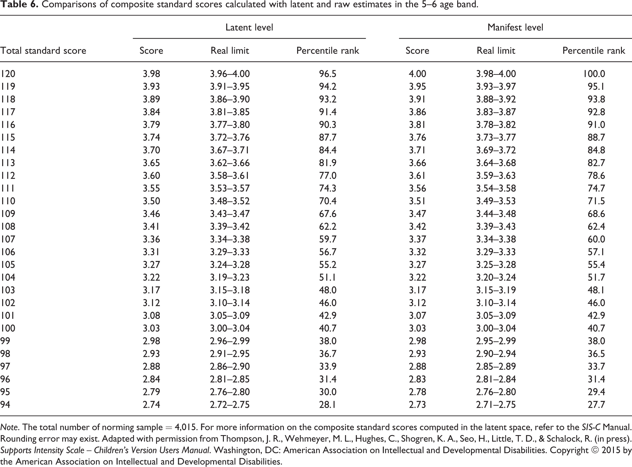
To obtain composite standard scores (i.e., SIS-C Support Needs Index) for each age group, we undertook the same procedures used to compute the subscale standard scores. First, Z scores were calculated with latent means and standard deviations obtained from the confirmatory factor analyses. Next, we obtained T scores of the overall support needs by applying a mean of 100 and a standard deviation of 15 (Thompson, Wehmeyer, et al., in press). Equations for these Z and T scores are provided in Figure 1. Percentile ranks were also reported to clarify the interpretation of raw scores (i.e., averaged subscale scores were the raw scores used to compute composite standard scores). Table 6 compares the composite standard scores (T scores), real limits, and percentile ranks in the 5–6 age band calculated at both latent and raw spaces. Differences were found between the two different approaches used.

Table 6.

Comparisons of composite standard scores calculated with latent and raw estimates in the 5–6 age band.

Total standard score	Latent level			Manifest level
Total standard score	Score	Real limit	Percentile rank	Score	Real limit	Percentile rank
120	3.98	3.96–4.00	96.5	4.00	3.98–4.00	100.0
119	3.93	3.91–3.95	94.2	3.95	3.93–3.97	95.1
118	3.89	3.86–3.90	93.2	3.91	3.88–3.92	93.8
117	3.84	3.81–3.85	91.4	3.86	3.83–3.87	92.8
116	3.79	3.77–3.80	90.3	3.81	3.78–3.82	91.0
115	3.74	3.72–3.76	87.7	3.76	3.73–3.77	88.7
114	3.70	3.67–3.71	84.4	3.71	3.69–3.72	84.8
113	3.65	3.62–3.66	81.9	3.66	3.64–3.68	82.7
112	3.60	3.58–3.61	77.0	3.61	3.59–3.63	78.6
111	3.55	3.53–3.57	74.3	3.56	3.54–3.58	74.7
110	3.50	3.48–3.52	70.4	3.51	3.49–3.53	71.5
109	3.46	3.43–3.47	67.6	3.47	3.44–3.48	68.6
108	3.41	3.39–3.42	62.2	3.42	3.39–3.43	62.4
107	3.36	3.34–3.38	59.7	3.37	3.34–3.38	60.0
106	3.31	3.29–3.33	56.7	3.32	3.29–3.33	57.1
105	3.27	3.24–3.28	55.2	3.27	3.25–3.28	55.4
104	3.22	3.19–3.23	51.1	3.22	3.20–3.24	51.7
103	3.17	3.15–3.18	48.0	3.17	3.15–3.19	48.1
102	3.12	3.10–3.14	46.0	3.12	3.10–3.14	46.0
101	3.08	3.05–3.09	42.9	3.07	3.05–3.09	42.9
100	3.03	3.00–3.04	40.7	3.03	3.00–3.04	40.7
99	2.98	2.96–2.99	38.0	2.98	2.95–2.99	38.0
98	2.93	2.91–2.95	36.7	2.93	2.90–2.94	36.5
97	2.88	2.86–2.90	33.9	2.88	2.85–2.89	33.7
96	2.84	2.81–2.85	31.4	2.83	2.81–2.84	31.4
95	2.79	2.76–2.80	30.0	2.78	2.76–2.80	29.4
94	2.74	2.72–2.75	28.1	2.73	2.71–2.75	27.7

Note. The total number of norming sample = 4,015. For more information on the composite standard scores computed in the latent space, refer to the SIS-C Manual. Rounding error may exist. Adapted with permission from Thompson, J. R., Wehmeyer, M. L., Hughes, C., Shogren, K. A., Seo, H., Little, T. D., & Schalock, R. (in press). Supports Intensity Scale – Children’s Version Users Manual. Washington, DC: American Association on Intellectual and Developmental Disabilities. Copyright © 2015 by the American Association on Intellectual and Developmental Disabilities.

Implications for future directions

The approach to norming that we have advocated here is relatively novel in the norming literature. As such, some researchers and stakeholders who are not well versed in the merits of latent variable modeling may hold undue skepticism regarding our procedures. However, the merits of latent variables are well established from various perspectives, including statistical theory and established practice in many fields of inquiry. A primary reason that SEM has not been used for norming purposes in the past has been the problem of scaling. The effects-coding method of identification that was introduced in 2006 provided a scaling method that retained the inherent metric of the observed scores. This one-to-one correspondence between the metric of the latent variables and the metric of the observed scores is the key that allows SEM to be used for norming purposes. Some users who are used to summing scores may find the use of average scores somewhat unfamiliar; however, the “learning curve” to use and interpret averages will be minimal because sums and averages are isomorphic regarding individual differences.

In terms of future directions, we suggest the widespread adoption of this approach to re-calibrate prior norms of other instruments. Accordingly, the approach we present here should become the new standard for norming continuous variable scales. The methods discussed above represent a very powerful and useful way to construct norms for continuously distributed data or data that closely approximates continuity (e.g., Likert-type items). When data are strictly categorical (e.g., binary testing items), however, IRT-based methods may represent more effective norming tools. This statement could be especially true when a rich understanding of the item-level measurement properties (e.g., individual item difficulty or discrimination abilities) is a necessary component of the norming context. Yet, in multidimensional cases, the methods we described here may still hold merit because multidimensional IRT (MIRT) is not as fully developed as methods for categorical variable SEM. Thus, future work should incorporate categorical indicators into the framework described above and compare the SEM-based approach we describe to IRT approaches (i.e., IRT true score equating), especially when there are differences in difficulty among alternative forms of a test. The case-study reported here was merely given as an example to demonstrate the strengths of SEM-based norming for social and behavioral researchers. Future research should employ simulation studies to rigorously explore the capabilities of SEM-based norming, particularly in comparison to IRT-based approaches.

Footnotes

Acknowledgements

The contributions of the first three authors on this article are equivalent. We wish to thank Carolyn Hughes, James R. Thompson, and Michael L. Wehmeyer for their assistance to develop this paper.

Funding

This study was supported in part by a grant from the U. S. Department of Education, Institute of Education Sciences, National Center for Special Education Research (Grant Award No. R324A120407). The opinions expressed do not necessarily reflect the position or policy of the Department of Education.

Appendix

References

Bodner

T. E.

(2006). Missing data: Prevalence and reporting practices. Psychological Reports, 99, 675−680.

Brown

T. A.

(2015). Confirmatory factor analysis for applied research (2nd ed.). New York: Guilford.

Cicchetti

(1994). Guidelines, criteria, and rules of thumb for evaluating normed and standardized assessment instruments in psychology. Psychological Assessment, 6, 284−290.

Dieher

Heaton

Miller

Grant

(1998). The Paced Auditory Serial Addition Task (PASAT): Norms for age, education, and ethnicity. Assessment, 5, 375−387.

Fan

Hancock

G. R.

(2012). Robust means modeling: An alternative to hypothesis testing of independent means under variance heterogeneity and nonnormality. Journal of Educational and Behavioral Science, 37, 137−156.

Green

S. B.

Thompson

M. S.

(2006). Structural equation modeling for conducting tests of differences in multiple means. Journal of Psychosomatic Medicine, 68, 706−717.

Honaker

King

Blackwell

(2011). Amelia II: A program for missing data. Journal of Statistical Software, 45, 1−47.

Kolen

(2006). Scaling and norming. In Brennan

(Ed.), Educational measurement (pp. 155−186). Westport, CT: American Council on Education and Praeger Publishers.

Kolen

Brennan

(2014). Test equating, scaling, and linking: Methods and practices (3rd ed.). New York, NY: Springer.

10.

Little

T. D.

(1997). Mean and covariance structures (MACS) analyses of cross-cultural data: Practical and theoretical issues. Multivariate Behavioral Research, 32, 53−76.

11.

Little

T. D.

(2013). Longitudinal structural equation modeling: Methodology in the social sciences. New York, NY: Guildford press.

12.

Little

T. D.

Jorgensen

T. D.

Lang

K. M.

Moore

E. W. G.

(2013). On the joys of missing data. Journal of Pediatric Psychology, 39(2), 151−162.

13.

Little

T. D.

Rhemtulla

Gibson

Schoemann

A. M.

(2013). Why the item versus parcels controversy needn’t be one. Psychological Methods, 18, 285−300.

14.

Little

T. D.

Slegers

D. W.

Card

N. A.

(2006). A non-arbitrary method of identifying and scaling latent variables in SEM and MACS models. Structural Equation Modeling, 13, 59−72.

15.

McDonald

R. P.

(1999). Test theory. Mahwah, NJ: Erlbaum.

16.

Muthén

L. K.

Muthén

B. O.

(2012). Mplus User’s Guide (7th ed.). Los Angeles, CA: Muthén & Muthén.

17.

Peugh

J. L.

Enders

C. K.

(2004). Missing data in educational research: A review of reporting practices and suggestions for improvement. Review of Educational Research, 74, 525−556.

18.

Powell

Mackrain

LeBuffe

(2007). Devereux early childhood assessment for infants and toddlers technical manual. Lewisville, NC: Kaplan.

19.

R Development Core Team. (2008). R: A language and environment for statistical computing. R Foundation for Statistical Computing, Vienna, Austria. ISBN 3-900051-07-0. Retrieved from http://www.R-project.org

20.

Shavelson

R. J.

(1996). Statistical reasoning for the behavioral sciences (3rd ed.). Boston, MA: Allyn and Bacon.

21.

Shogren

Seo

Wehmeyer

Thompson

J.R.

Hughes

Little

Palmer

(in press). Support needs of children with intellectual and developmental disabilities: Age-related implications for assessment. Psychology in the Schools.

22.

Thompson

J. R.

Bradley

V. J.

Buntinx

W. H. E.

Schalock

R. L.

Shogren

K. A.

Snell

M. E.

… Wehmeyer

M. L.

(2009). Conceptualizing supports and the support needs of people with intellectual disability. Intellectual and Developmental Disabilities, 47, 135−146.

23.

Thompson

J. R.

Bryant

B. R.

Campbell

E. M.

Craig

E. M.

Hughes

C. M.

Rotholz

D. A.

… Wehmeyer

(2004). Supports Intensity Scale (SIS). Washington, DC: American Association on Mental Retardation.

24.

Thompson

J. R.

Bryant

B. B.

Schalock

R. L.

Shogren

K. A.

Tassé

M. J.

Wehmeyer

M. L.

… Silverman

W. P.

(2015). Supports Intensity Scale – Adult Version Users Manual. Washington, DC: American Association on Intellectual and Developmental Disabilities.

25.

Thompson

J. R.

Wehmeyer

M. L.

Hughes

Shogren

K. A.

Little

T. D.

Copeland

S. R.

… Tassé

M. J.

(in press). Supports Intensity Scale − Children’s Version. Washington, DC: American Association on Intellectual and Developmental Disabilities.

26.

Tombaugh

(2004). Trail making test A and B: Normative data stratified by age and education. Archives of Clinical Neuropsychology, 19, 203−214.

27.

Wechsler

(2014). Wechsler Intelligence Scale for Children − Fifth Edition. San Antonio, TX: NCS Pearson.