The Parallel Declines of Intergenerational Economic Mobility and Marriage: Are They Related?

Abstract

Intergenerational mobility declined in the second half of the 20th century—simultaneously with the decline in marriage rates and the rise of single parenthood. This study investigated whether county-level intergenerational mobility rates predict family formation patterns. We utilized a county-level measure of intergenerational mobility constructed by Chetty and Hendren for a cohort of young adults born between 1980 and 1986 and raised in lower-income families, merged with county-level rates of marriage and single parenthood from the 2015–2019 American Community Survey 5-year estimates. Regression models showed that higher intergenerational mobility is associated with subsequent higher marriage rates while lower intergenerational mobility is associated with subsequent higher rates of single parenthood. These results provide descriptive evidence that the decline in intergenerational mobility seen during the second half of the 20th century may be one of the drivers of the decline in marriage and the rise of single parenthood seen during the same era.

Keywords

family structure intergenerational economic mobility low-income families marriage single parenthood

Introduction

Intergenerational mobility in the United States has been on the decline since the second half of the 20th century (Aaronson & Mazumder, 2008; Davis & Mazumder, 2024; Jácome et al., 2021). While families may still hope that children will earn more and have a higher standard of living compared to their parents, the likelihood of this actually happening has fallen from 90 percent for children born in the 1940s to about 50 percent for children born in the 1980s—a trend dubbed by economist Raj Chetty and colleagues as “the fading American dream” (Chetty et al., 2017).

Simultaneously, the retreat from marriage in both the 20th and 21st centuries has been profound. Today, fewer than 50 percent of American adults are married, an historic low. Further, today more U.S. children live apart from one of their biological parents than children in any other rich nation (Gornick et al., 2022b). Though marital stability has increased among parents who do marry, more than one in four children grow up in single parent households, due largely to declining marriage rates (Federal Interagency Forum on Child and Family Statistics, 2023).

Decreases in marriage and increases in single parenthood have been more marked among the less advantaged. Adults with at least a bachelor’s degree are 15 percentage points more likely to be married than their counterparts without a high school education (Parker & Stepler, 2017). Those with less education are less likely to marry at all and more likely to divorce if they do marry. Further, while fully 75 percent of non-Hispanic white children lived in marital households in 2022, only about 60 percent of their Hispanic counterparts and 38 percent of their non-Hispanic Black counterparts did so (Federal Interagency Forum on Child and Family Statistics, 2023). This is despite the fact that disadvantaged Americans continue to aspire to marriage, as a substantial body of both survey and qualitative research has shown (Edin & Kefalas, 2011; Edin & Nelson, 2013; Edin & Reed, 2005; Gibson-Davis et al., 2005; Waller & McLanahan, 2005).

In this study, we examine the relationships between a county-level measure of intergenerational mobility for children born in the early- to mid-1980s and raised in the 25th percentile of income rank when they reach young adulthood (age 26), and that county’s rates of marriage and single parenthood (measured in 2019). Recent causal evidence from Chetty & Hendren (2018) suggests that individual-level mobility is, to a significant degree, shaped by the communities in which young people are raised. We use counties, rather than census tracts, as our unit of analysis because we seek to understand the large variation in marriage and single parenthood rates regionally, including in the vast swaths of the nation that are rural. Rates of marriage and single parenthood vary dramatically across regions, as this paper will show.

With marriage rates at an historic low, especially among the poor and working class, young people’s ability to achieve intergenerational mobility might well have become highly consequential for family formation. In sum, we hypothesize that when more individuals within a community are able to economically advance beyond their parents, more will marry and fewer will raise their children alone, and when more individuals are economically level with or worse off than their parents, fewer will marry and more will raise their children alone.

Background

Over the last quarter of the 20th century, a highly influential hypothesis was advanced regarding the role of economic conditions in declining marriage rates. Wilson’s (1987) landmark book, The Truly Disadvantaged, argued that, due to the relocation of job opportunities from inner-city Black neighborhoods to the suburbs and the Sunbelt, there were simply too few marriageable Black men to go around (called the “Male Marriageable Pool Hypothesis” or the “Male Marriageable Pool Index,” an idea first advanced by Wilson & Neckerman, 1987).

Subsequent to Wilson’s book, a large body of quantitative literature emerged examining the role of economic conditions on family structure. Most sociological and demographic studies have focused on the relationship between economic characteristics and family formation outcomes at the individual level, including testing the contemporary relevance of the Male Marriageable Pool Hypothesis. For example, one study explored the economic characteristics (e.g., education, employment status, and income) that would likely deem a “hypothetical husband” to be marriageable using data from the 2008–2012 and 2013–2017 American Community Surveys (Lichter et al., 2020). Compared to the unmarried men in the study sample, the “hypothetical husbands” had higher incomes, were more likely to have college degrees, and were more likely to be employed. A similar study used data from the Future of Families and Child Wellbeing Study to compare the characteristics of men who had children with young single mothers (ages 18–21) with those of men who had children with women who were older than 21 years of age and, separately, with those of men who were married (Lopoo & Carlson, 2008). The partners of young single mothers were less likely to meet the economic characteristics of marriageability—they were less likely to be employed or attending school—compared to the other men in the sample. The results from both of these analyses suggest that there is indeed a dearth of marriageable men, based on broadly defined economic characteristics.

Drawing on a number of qualitative studies in the 2000s (Edin & Kefalas, 2011; Gibson-Davis et al., 2005), scholars further advanced Wilson’s hypothesis by suggesting that men were deemed “marriageable” when they met a specific economic bar. For example, one study explored whether couples achieved seven specific indicators of economic stability (i.e., steady employment, earnings growth, health insurance coverage, home ownership, being banked, avoiding welfare receipt, avoiding material hardship) during the year-long Building Strong Families intervention (Gibson-Davis et al., 2018). The authors found that couples who met at least four of these economic indicators were significantly more likely to marry—in line with the notion of a marriage bar.

A second example used individual-level data from the 1980–2000 U.S. censuses to show that men with incomes below the local median—defined as the median income of a fully employed man living in a specific metropolitan area—were more likely to marry after they experienced income growth (Watson & McLanahan, 2011; see also: Ishizuka, 2018). Men whose incomes fell below the local median had lower likelihood of being married. Interestingly, local median income and marriage likelihood were not related among men with incomes above the local median, suggesting that relative income within a community is specifically influential for marriage rates among those with lower incomes (Watson & McLanahan, 2011). Another study took a similar approach, examining whether income inequality within counties was associated with non-marital first births (Cherlin et al., 2016). Data from the National Longitudinal Survey of Youth 1997 cohort (NLSY-1997) showed that greater income inequality at the county level was associated with higher likelihood of a non-marital first birth among both young women and young men. Both of these studies suggest that local economic conditions have a significant impact on individual-level family formation behaviors.

Complementing this literature focused on individual-level outcomes, several studies have considered both economic factors and family formation outcomes at an aggregate level (i.e., counties, public-use microdata areas [PUMAs], commuting zones). The first such study demonstrated that the positive economic shock of the Appalachian “coal boom” in the 1970s was associated with higher marital birth rates in counties that experienced the coal boom (Black et al., 2013). Revisiting the findings of this study, a second study demonstrated that the increased earnings associated with the 1970s coal boom led to an increase in marriage rates and a decrease in non-marital births in PUMAs that experienced the coal boom (Kearney & Wilson, 2018). This work additionally examined the positive economic shock of the “fracking boom” in the 2000s, finding that economic stimulation resulting from the fracking boom at the PUMA level was associated with increases in both marital and non-marital birth rates in that PUMA, but was not associated with marriage rates (Kearney & Wilson, 2018). In contrast, a third study demonstrated that at the commuting zone level, manufacturing decline—a major negative economic shock in many regions of the United States between 1990 and 2014—was associated with a lower proportion of women who were ever married, as well as a higher proportion of children living in single-parent households (Autor et al., 2019). This small literature provides evidence that economic conditions—specifically, exogenous economic shocks—in a community or geographic area are associated with family formation behaviors among the local population.

In sum, the extant literature has shown strong associations between individual and local economic conditions and individual family formation outcomes, as well as strong associations between regional economic shocks and family formation patterns among the affected population(s). This body of evidence has led us to a related yet novel research question: are local economic conditions (not limited to a specific economic shock) similarly associated with subsequent family formation patterns in the local population? We approach this broad question by focusing on an important economic outcome—intergenerational mobility. We examine whether intergenerational mobility, captured when young people are entering their prime family building years, is associated with subsequent family formation patterns at the county level, in total and for various subgroups. Specifically, we ask: does the rate of intergenerational mobility in a community predict family formation patterns in that community, all else equal?

We examine this question using county-level measures for two reasons. First, work by Chetty & Hendren (2018) demonstrates that community context, as measured at the county level, is strongly predictive of individual outcomes. Second, focusing on counties—rather than PUMAs, metropolitan statistical areas, or commuting zones—allows us to include rural America, for which the county is the most salient jurisdictional boundary (Tolnay & Beck, 1995; see also: Mann et al., 2024). As we will show, rural counties, particularly those in the South, have some of the lowest rates of intergenerational mobility in the nation, along with some of the lowest marriage rates.

Methods

Data

This study primarily utilized pooled data from the 2015–2019 American Community Survey 5-year estimates (henceforth: 2019 ACS; U.S. Census Bureau, 2024). We considered county-level data on marriage and single-parent households. The ACS also includes rich socioeconomic data, including county-level data on poverty rate, unemployment rate, racial and ethnic makeup, and sex ratio.

Measures

Predictor of Interest

The predictor of interest in this study was a county-level measure of intergenerational mobility among children raised in low-income families when they reached their prime family building years. This measure was constructed by Chetty, Hendren, and colleagues to capture a county’s average income rank at age 26 for individuals born between 1980 and 1986 whose parents were in the 25th percentile of the national income distribution when the individuals themselves were in middle childhood (i.e., between 1996 and 2000; Chetty et al., 2014). The data used to construct this measure were drawn from federal income tax returns (1040 and W-2 forms). This measure describes the mean level of intergenerational economic mobility, measured by income rank in early adulthood, for children who were raised in low-income families with an income rank at the 25th percentile. We focused on mobility among those raised in low-income households because of the large literature indicating that marriage rates are lower—and rates of single parenthood are higher—among individuals and households with lower incomes (Livingston, 2018; Parker & Stepler, 2017). This particular measure has been widely used in previous research about intergenerational mobility in the United States (Chetty et al., 2014; Connolly & Haeck, 2024; Jácome et al., 2021) and will allow us to test the hypothesis that intergenerational mobility is consequential for family formation, especially among households with lower incomes.

As robustness checks, we considered the county-level intergenerational mobility measure for four demographic subgroups: male residents, female residents, Black residents, and white residents, allowing us to examine whether specific mobility rates by sex or race are associated with county-level family formation outcomes.

Outcome Variables

We focused on two outcomes of interest constructed from the 2019 ACS: county-level marriage rate and county-level rate of single-parent households. The county-level marriage rate included the number of adults ages 15 and over who were either currently married or married but with an absent spouse for “other reason” (but not separated) at the time of the 2019 ACS, divided by the total number of county residents ages 15 and over. The county-level rate of single-parent households included the number of households with children under the age of 18 with either a male or female householder with no spouse present at the time of the 2019 ACS, divided by the total number of households in the county with children under the age of 18.

We constructed three alternate marriage outcomes for robustness checks to determine whether associations between intergenerational mobility and marriage differed based on age group, educational attainment, or income of residents. The first alternate marriage outcome included the number of adults ages 30–39 who were either currently married or married with an absent spouse for “other reason” (not separated) at the time of the 2019 ACS, divided by the total number of county residents ages 30–39 (and, for comparison, we computed the same measure among adults ages 40 and over). This age range (30–39) is roughly commensurate with the ages of the Chetty-Hendren cohort in 2019. The second alternate marriage outcome included the number of married heads of household who have a high school diploma or less education, divided by the total number of heads of household in the county who have a high school diploma or less education (and the higher-educated inverse for comparison). The third alternate marriage outcome included the number of married heads of household with incomes below 185% of the federal poverty level (FPL), divided by the total number of households in the county with incomes below 185% FPL (and the higher-income inverse for comparison).

We also constructed one alternate single-parent household outcome for a robustness check to determine whether associations between intergenerational mobility and single parenthood differed based on residents’ income. The alternate single-parent household outcome included the number of single-parent households (with children under 18) with incomes below 185% FPL, divided by the total number of households with children under 18 in the county with incomes below 185% FPL (and the higher-income inverse for comparison).

Covariates

We adjusted for several sociodemographic covariates potentially related to marriage and single parenthood, also drawn from the 2019 ACS, to mirror the outcome variables. County-level covariates included the proportion of households with incomes below the FPL (“poverty”); the proportion of adults in the labor force who were unemployed (“unemployment”); the proportion of adults ages 25 and over who had graduated from college (“college graduates”); the sex ratio, specifically the proportion of males among adults ages 15 and over (“males”); the median income among males and females ages 16 and over who were employed full-time for the past 12 months (“median male income” and “median female income,” respectively); the average age of residents (“average age”); the average age of residents, squared (“age squared”); the proportion of residents who were non-Hispanic Black (“non-Hispanic Black”); the proportion of residents who were non-Hispanic other race, including Asian, American Indian or Alaska Native, and Native Hawaiian or Pacific Islander (“non-Hispanic other race”); the proportion of residents who were Hispanic (“Hispanic”); and the proportion of residents who were born outside of the United States (“foreign born”).

In select regression models, we adjusted for a lagged predictor from the 1980 decennial census corresponding to the outcome of interest: (a) the number of adults ages 15 and over who were married at the time of the 1980 census, divided by the number of county residents ages 15 and over (“adults married in 1980”); and (b) the number of households with children under the age of 18 with either a male or female householder with no spouse present at the time of the 1980 census, divided by the total number of households with children under the age of 18 (“single-parent households in 1980”).

Finally, in select regression models, we adjusted for several predictors that, together, served as proxies for out-migration, as selective migration out of communities may be impactful to county-level outcomes. This set of predictors included (a) total county population change between 2018 and 2019; (b) the percentage of households that lived in the same house or apartment in 2018 and 2019; and (c) the median number of years that residents lived at their current addresses as of 2019.

Analytic Approach

We began by describing the data and examining bivariate correlations between all variables of interest. We then used a series of multivariable ordinary least squares (OLS) regression models, correcting for heteroskedasticity with White’s robust standard errors, and adjusting for multiple hypothesis testing using Hommel corrections (Hommel, 1988). The intergenerational mobility predictors were unstandardized in all regression models for ease of comparison across models, while all covariates were standardized (subtracted from their mean value and divided by their standard deviation) in all regression models. The first pair of models (Model 1a and Model 2a) estimated the relationships between intergenerational mobility and the two outcomes of interest: marriage rate and rate of single-parent households, respectively, adjusting for a broad set of county-level covariates:

(M o d e l 1 a) {M A R R}_{i} = β_{0} + β_{im} {(I M)}_{i} + β_{c} {(C T R L)}_{i} + Ɛ_{i}

(M o d e l 2 a) {S I N G L E}_{i} = β_{0} + β_{im} {(I M)}_{i} + β_{c} {(C T R L)}_{i} + Ɛ_{i}

MARR represents the marriage rate and SINGLE represents the rate of single-parent households, the respective outcomes of interest in these two models, while i represents the county. IM represents intergenerational mobility. CTRL represents the set of sociodemographic covariates described in more detail in the Methods section.

Building on Model 1a and Model 2a, we adjusted Model 1b and Model 2b for lagged predictors of marriage rate [PASTMARR] and rate of single-parent households [PASTSING], respectively, derived from the 1980 decennial census; these two lagged predictors correspond to the two outcomes of interest from 2019. Model 1b and Model 2b were also adjusted for state fixed effects to account for state-level variation in underlying rates of marriage that may be correlated with the outcomes of interest, as well as CTRL. Then, further building on Model 1b and Model 2b, we additionally adjusted Model 1c and Model 2c for the three predictors related to population change and out-migration from counties [OUTMIG]. Model 1c and Model 2c were also adjusted for state fixed effects, as well as CTRL.

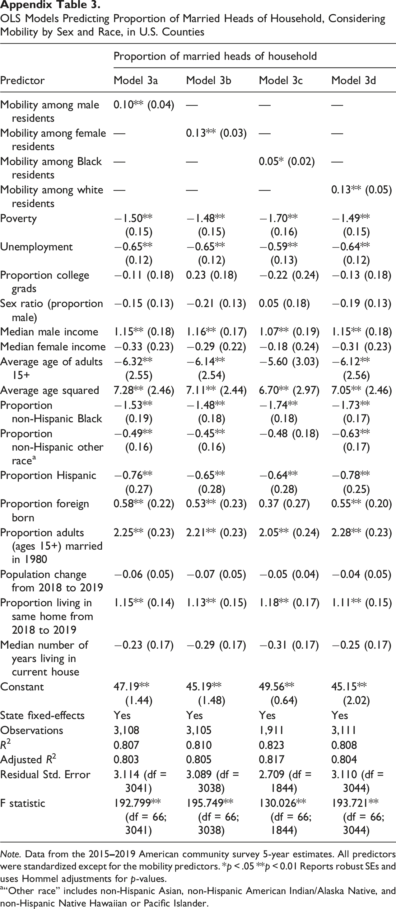
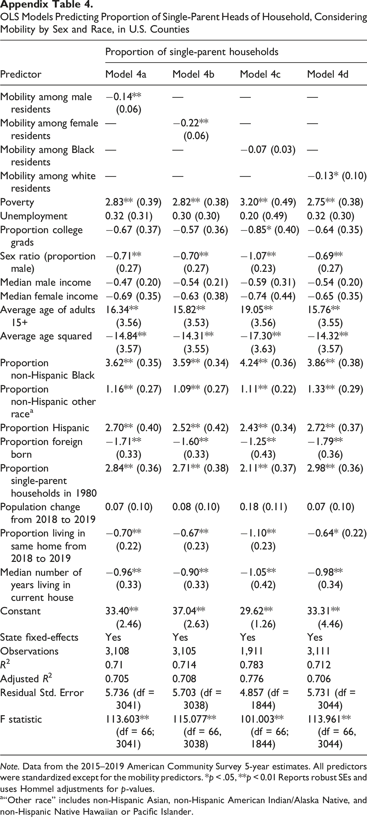
We then conducted several robustness checks. In the first robustness check, we considered several alternate predictors of interest, specifically exploring intergenerational mobility by sex and race, as described in the Methods section. As these models explored relationships between these alternate predictors of interest and the main outcomes, these models were adjusted for PASTMARR or PASTSING, corresponding to the outcome, as well as CTRL, OUTMIG, and state fixed effects. We explored whether the relationships between intergenerational mobility and the outcomes of interest were robust considering mobility among male residents and, separately, mobility among female residents using outcomes representing the marriage rate (Models 3a and 3b, respectively) and the rate of single-parent households (Models 4a and 4b, respectively), by county. We then investigated whether the relationships between intergenerational mobility and the outcomes of interest were robust considering intergenerational mobility among Black residents and, separately, intergenerational mobility among white residents using outcomes representing the marriage rate (Models 3c and 3d, respectively) and the rate of single-parent households (Models 4c and 4d, respectively), by county. As some counties had few or no Black residents, intergenerational mobility among Black residents could not be computed for all counties; thus, a sub-sample of counties were included in these analyses.

Additional robustness checks utilized alternate marriage and single parenthood outcomes, as described in the Methods section. The remaining robustness checks included IM as the predictor of interest and adjusted for CTRL, OUTMIG, and state fixed effects. Note that these models did not adjust for PASTMARR or PASTSING as we were unable to create lagged predictors for specific sociodemographic groups due to limitations with the 1980 census data. The second robustness check focused on individuals around the age of the Chetty-Hendren cohort in their prime marrying and childbearing years by considering the marriage rate in 2019 among adults ages 30–39 (Model 5a). In a complementary model, we considered all individuals who were older than the Chetty-Hendren cohort at the time of the 2019 ACS by focusing on adults who were ages 40 and over (Model 5b). We were unable to compute the rate of single parenthood among specific age groups due to data limitations.

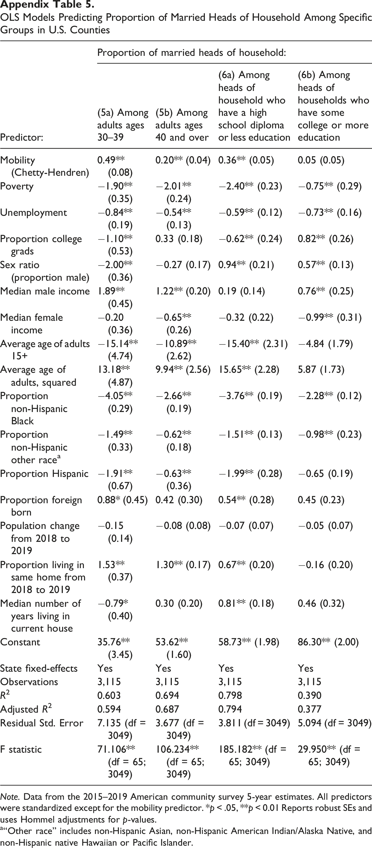
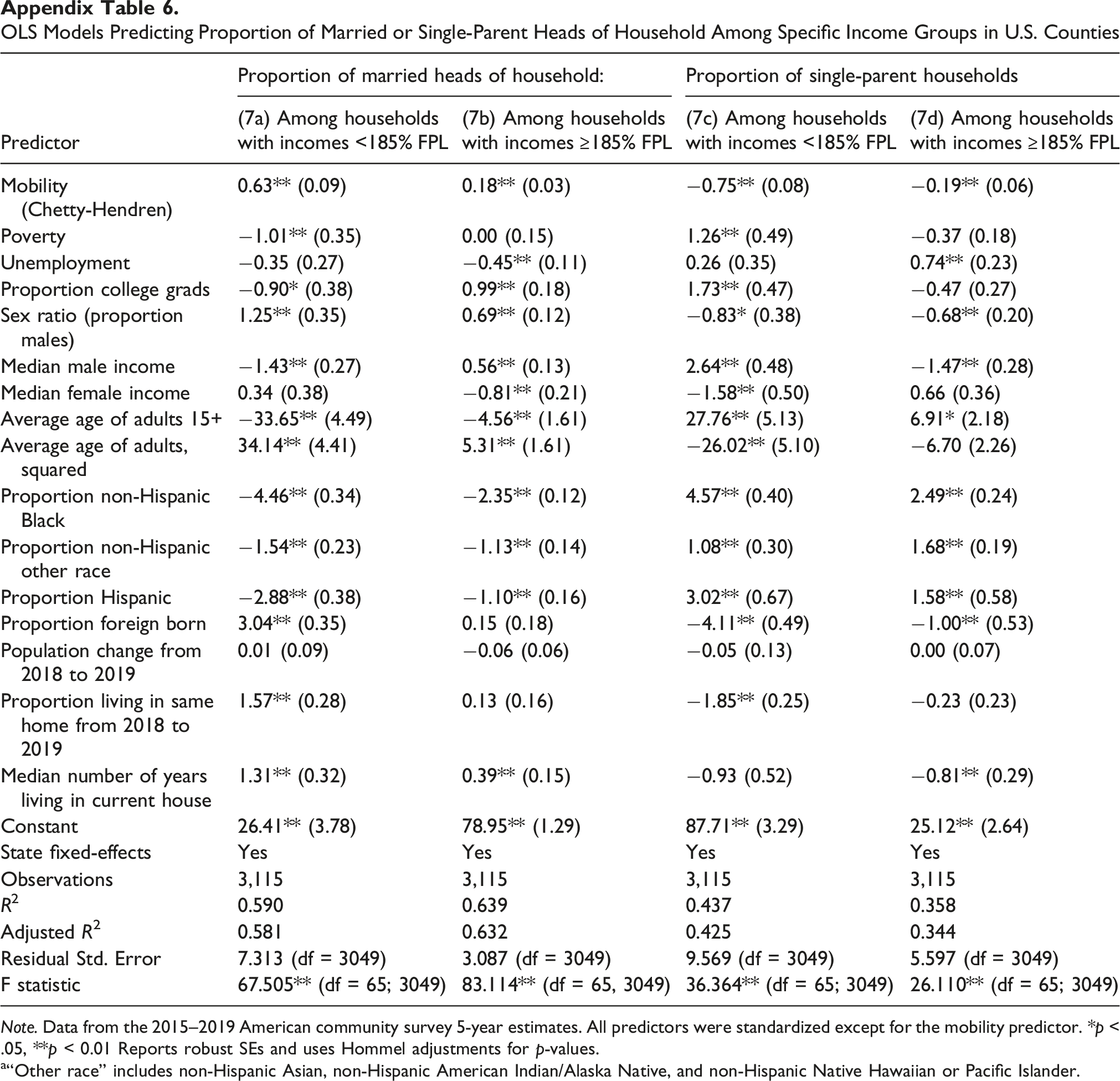
The third robustness check considered whether the relationship between intergenerational mobility and marriage rate was robust among heads of household with less education (high school diploma or less—the group least likely to marry) and, separately, among heads of household with more education (some college or more) using outcomes representing the marriage rate within each group (Models 6a and 6b, respectively). Again, the proportion of single parents among heads of household based on educational attainment was unable to be computed using the 2019 ACS; thus, we only implemented these robustness checks for the marriage rate outcome. In the final robustness check, we considered whether the relationships between intergenerational mobility and the outcomes of interest were robust among households with different incomes. We used outcomes representing the marriage rate among the lower and higher income groups (Models 7a and 7b, respectively) and the rate of single-parent households among the lower and higher income groups (Models 7c and 7d, respectively).

Results

Descriptive Statistics

First, we described the data by examining the means of all variables of interest, mapping the rates of intergenerational mobility and the two outcomes of interest across counties in the United States, and exploring correlations between all variables of interest. The descriptive statistics shown in Appendix 1 allow us to consider an average county in the United States in 2019: individuals who were low-income as children reached the 45.9 percentile income rank in early adulthood; 51.4% of adults ages 15 and over were married; and 29.9% of households with children were headed by single parents in this average county.

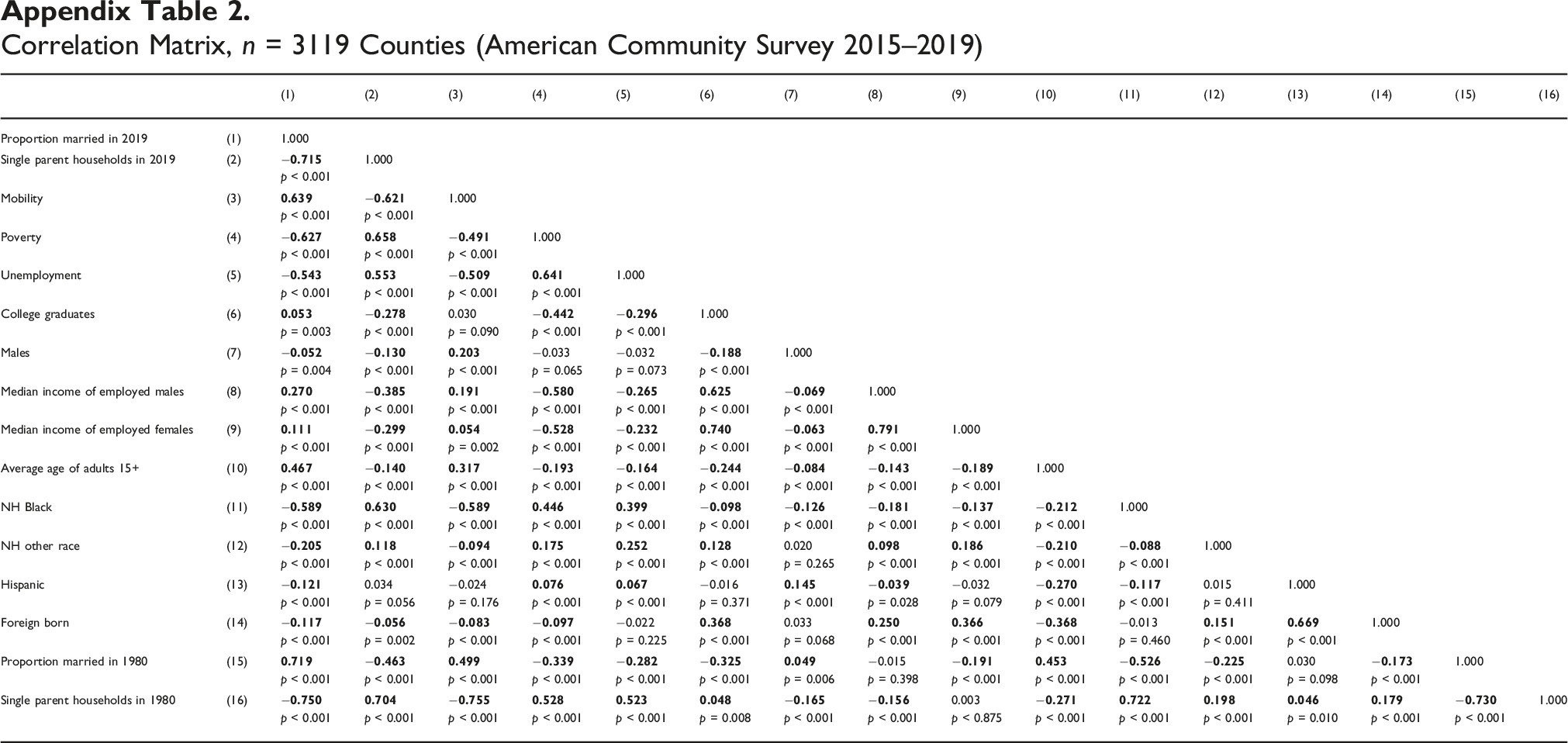
One of the goals of this analysis was to better understand the marked regional variation in marriage and single parenthood rates across the United States. Figure 1 shows variation in intergenerational mobility and marriage rates across U.S. counties, reflecting the strong correlation between intergenerational mobility and marriage (r = 0.64, p < 0.001; see Appendix Table 2). Figure 2 shows variation in intergenerational mobility and rates of single parent households across counties, similarly reflecting the strong correlation between these two variables (r = −0.62, p < 0.001; see Appendix Table 2). In each map, counties are categorized by low, medium, or high rates of intergenerational mobility, as well as low, medium, or high rates of marriage or single parenthood.

Figure 1.

Variation in intergenerational mobility and marriage across U.S. counties

Figure 2.

Variation in intergenerational mobility and households headed by single parents across U.S. counties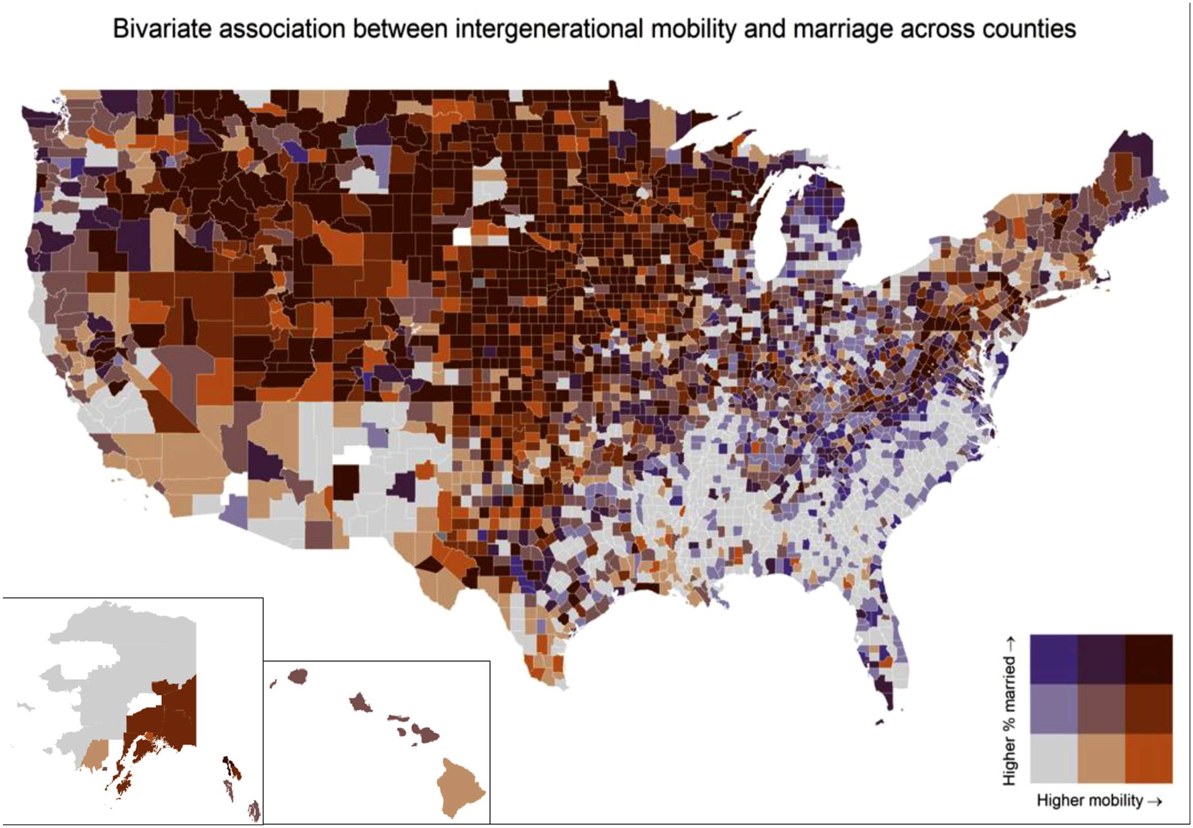

Consistent with our hypothesis, many counties in the low-intergenerational mobility Deep South have subsequent marriage rates that are much lower, and single parenthood rates that are much higher, than in the rest of the country (counties shaded gray in Figures 1 and 2, respectively). Counties in the upper Midwest and Mountain West, on the other hand, show the opposite pattern (counties shaded dark maroon in Figure 1, dark green in Figure 2). Exceptions to these regional patterns include Appalachia and parts of the Bible Belt (the upper South/lower Midwest), where marriage rates remain high and single parenthood rates are low despite limited intergenerational mobility, and parts of New England, where intergenerational mobility is average, yet marriage rates are relatively low and single parenthood rates are high. Overall, only a small proportion of counties display trends contrary to our hypothesis: the combinations of low intergenerational mobility and high marriage rate; high intergenerational mobility and low marriage rate; low intergenerational mobility and low rate of single parenthood; and high intergenerational mobility and high rate of single parenthood are each seen in about 3% of counties.

Intergenerational Mobility, Marriage, and Single Parenthood

Moving into the findings from our OLS regression models, results from Models 1a and 2a are presented in Table 1. In Model 1a, intergenerational mobility was significantly associated with subsequent county-level rates of marriage (B = 0.26, p < 0.01). In Model 2a, as with marriage, intergenerational mobility was significantly associated with subsequent county-level rates of single parenthood (B = −0.43, p < 0.01).

Table 1.

OLS Models Predicting Proportion of Married or Single Parent Heads of Household in U.S. Counties

Predictor	Proportion of married heads of household			Proportion of single parent heads of household
Predictor	Model 1a	Model 1b	Model 1c	Model 2a	Model 2b	Model 2c
Mobility (Chetty-Hendren)	0.26** (0.02)	0.15** (0.04)	0.13** (0.04)	−0.43** (0.03)	−0.30** (0.07)	−0.23** (0.07)
Poverty	−2.22** (0.17)	−1.54** (0.17)	−1.48** (0.15)	3.16** (0.27)	2.71** (0.39)	2.82** (0.38)
Unemployment	−0.75** (0.12)	−0.63** (0.13)	−0.63** (0.12)	0.57** (0.21)	0.37 (0.33)	0.33 (0.31)
Proportion college grads	−1.13** (0.16)	−0.24 (0.15)	−0.08 (0.17)	−0.09 (0.22)	−0.17 (0.38)	−0.60 (0.37)
Sex ratio (proportion males)	−1.00** (0.10)	−0.70** (0.11)	−0.19 (0.13)	−0.36* (0.16)	−0.38** (0.24)	−0.67** (0.28)
Median male income	1.40** (0.17)	1.17** (0.18)	1.11** (0.17)	−1.03** (0.25)	−0.68* (0.20)	−0.54 (0.19)
Median female income	−1.12** (0.20)	−0.22 (0.24)	−0.34 (0.23)	0.55* (0.30)	−0.77* (0.32)	−0.67 (0.34)
Average age of adults 15+	−0.36 (2.72)	−4.53** (2.54)	−6.00** (2.55)	14.58** (2.72)	11.66** (3.94)	16.23** (3.62)
Average age of adults, squared	1.82 (2.67)	5.78** (2.47)	6.96** (2.45)	−13.60** (2.73)	−10.98** (4.02)	−14.74** (3.64)
Proportion non-Hispanic Black	−1.92** (0.10)	−1.39** (0.21)	−1.47** (0.19)	3.86** (0.18)	3.19** (0.37)	3.60** (0.34)
Proportion non-Hispanic other race^a	−0.39** (0.08)	−0.26 (0.15)	−0.46** (0.16)	1.09** (0.19)	0.65** (0.24)	1.09** (0.26)
Proportion Hispanic	−0.68** (0.19)	−0.54** (0.30)	−0.72** (0.28)	1.53** (0.25)	1.95** (0.31)	2.56** (0.39)
Proportion foreign born	0.57** (0.16)	0.59** (0.23)	0.55** (0.22)	−1.06** (0.23)	−1.38** (0.30)	−1.61** (0.32)
Proportion adults (ages 15+) married in 1980	—	2.55** (0.22)	2.25** (0.24)	—	—	—
Proportion single parent households in 1980	—	—	—	—	2.94** (0.43)	2.63** (0.38)
Population change from 2018 to 2019	—	—	−0.06 (0.05)	—	—	0.07 (0.10)
Proportion living in same home from 2018 to 2019	—	—	1.14** (0.15)	—	—	−0.66** (0.23)
Median number of years living in current house	—	—	−0.26 (0.17)	—	—	−0.90** (0.34)
Constant	39.48** (0.97)	44.96** (1.64)	45.40** (1.64)	49.81** (1.51)	39.95** (2.98)	37.26** (3.03)
State fixed-effects	No	Yes	Yes	No	Yes	Yes
Observations	3,117	3,117	3,117	3,117	3,117	3,117
R ²	0.697	0.796	0.807	0.644	0.706	0.713
Adjusted R²	0.696	0.792	0.803	0.643	0.700	0.707
Residual Std. Error	3.878 (df = 3103)	3.208 (df = 3053)	3.122 (df = 3048)	6.325 (df = 3103)	5.798 (df = 3053)	5.724 (df = 3048)
F statistic	548.641** (df = 13; 3103)	188.915** (df = 63; 3053)	192.845** (df = 66; 3048)	432.362 (df = 13; 3103)	116.348** (df = 63; 3053)	114.837** (df = 66; 3048)

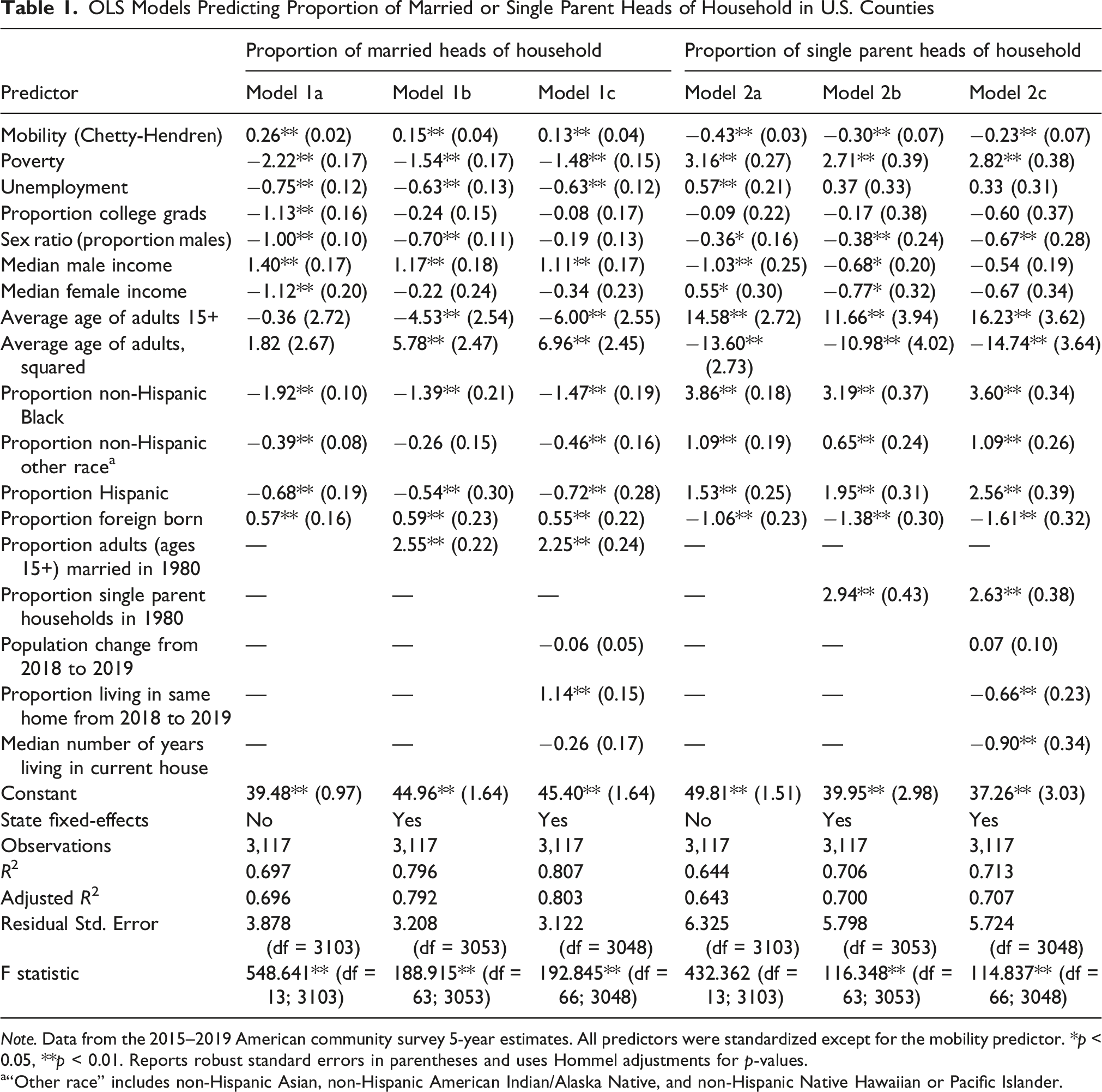
Note. Data from the 2015–2019 American community survey 5-year estimates. All predictors were standardized except for the mobility predictor. *p < 0.05, **p < 0.01. Reports robust standard errors in parentheses and uses Hommel adjustments for p-values.

^a“Other race” includes non-Hispanic Asian, non-Hispanic American Indian/Alaska Native, and non-Hispanic Native Hawaiian or Pacific Islander.

We further explored the relationships between intergenerational mobility and family formation outcomes after adjusting for regional patterns in family formation in the year 1980—around the time that the parents of the cohort represented in the Chetty-Hendren data were in their childbearing years. Results of Models 1b and 2b are also shown in Table 1. In Model 1b, the association between intergenerational mobility and marriage remained statistically significant (B = 0.15, p < 0.01). We also see that the marriage rate in 1980 was significantly associated with the marriage rate in 2019 (B = 2.55, p < 0.01), even adjusting for state fixed effects. Further, in Model 2b, the association between intergenerational mobility and the rate of single parenthood remains statistically significant (B = −0.30, p < 0.01). The rate of single parenthood in 1980 was also significantly related to the rate of single parenthood in 2019, all else equal (B = 2.94, p < 0.01).

We also considered that selective migration out of counties may impact family formation outcomes, as well as the relationships between intergenerational mobility and family formation outcomes. Results of Models 1c and 2c are also shown in Table 1. In Model 1c, the association between intergenerational mobility and marriage remained statistically significant (B = 0.13, p < 0.01). However, only one of the three proxies for out-migration—the proportion of householders living in the same home from 2018 to 2019—was significantly associated with the marriage rate (B = 1.14, p < 0.01). In Model 2c, the association between intergenerational mobility and single parenthood retained statistical significance (B = −0.23, p < 0.01). Further, two of the three proxies for out-migration were significantly associated with single parenthood: the proportion of householders living in the same house from 2018 to 2019 (B = −0.66, p < 0.01) and the median number of years that householders lived at their current addresses (B = −0.90, p < 0.01).

Robustness Check: Exploring Intergenerational Mobility by Sex and Race

We recognize that the associations between intergenerational mobility and county-level rates of marriage and single parenthood may vary among different sociodemographic groups. First, Wilson’s Male Marriageable Pool Hypothesis suggests that intergenerational mobility among women may be less important than intergenerational mobility among men for marriage and, conversely, single parenthood. However, a more recent literature, drawing on immersive interviews with low-income women, suggests that in a more contemporary era, women too must meet a certain economic threshold in order to be considered marriageable, either by their partners or by themselves (Bell et al., 2018; Edin & Nelson, 2013). Additionally, the work of Cross (2020) suggests that the association between intergenerational mobility and marriage (and, conversely, single parenthood) may be weaker among Black adults than among white adults, in part because marriage may confer fewer benefits for child wellbeing in some domains, and single parenthood may confer fewer risks.

We conducted several robustness checks to investigate any such variation; the key results of Models 3a–3d and Models 4a–4d are shown in Table 2 (full results presented in Appendix Tables 3 and 4). When we separately considered the associations between intergenerational mobility and family formation outcomes among male and female residents, all associations were significant, and intergenerational mobility was positively related to marriage rate (Models 3a and 3b) and negatively related to single parenthood rate (Models 4a and 4b). Note that the effect sizes were similar when we considered intergenerational mobility among male versus female residents. However, the effect sizes were substantially different when we considered intergenerational mobility among white residents compared to intergenerational mobility among Black residents. The association was significant in both models exploring intergenerational mobility among white residents, but in only one model exploring intergenerational mobility among Black residents, in line with Cross’s work (2020). Further, the coefficients representing the associations between intergenerational mobility and marriage (Models 3c and 3d) and single parenthood (Models 4c and 4d) were more than twice as large among white residents than Black residents.

Table 2.

OLS Models Predicting Proportion of Married or Single Parent Heads of Household, Considering Mobility by Sex and Race, in U.S. Counties

Predictor	Proportion of married heads of household
Predictor	Model 3a	Model 3b	Model 3c	Model 3d
Mobility among male residents	0.10** (0.04)	—	—	—
Mobility among female residents	—	0.13** (0.03)	—	—
Mobility among Black residents	—	—	0.05* (0.02)	—
Mobility among white residents	—	—	—	0.13** (0.05)
Constant	47.19** (1.44)	45.19** (1.48)	49.56** (0.64)	45.15** (2.02)
R ²	0.807	0.810	0.823	0.808
Adjusted R²	0.803	0.805	0.817	0.804

Predictor	Proportion of single parent heads of household
Predictor	Model 4a	Model 4b	Model 4c	Model 4d
Mobility among male residents	−0.14** (0.06)	—	—	—
Mobility among female residents	—	−0.22** (0.06)	—	—
Mobility among Black residents	—	—	−0.07 (0.03)	—
Mobility among white residents	—	—	—	−0.13* (0.10)
Constant	33.40** (2.46)	37.04** (2.63)	29.62** (1.26)	33.31** (4.46)
R ²	0.711	0.714	0.783	0.712
Adjusted R²	0.705	0.708	0.776	0.706

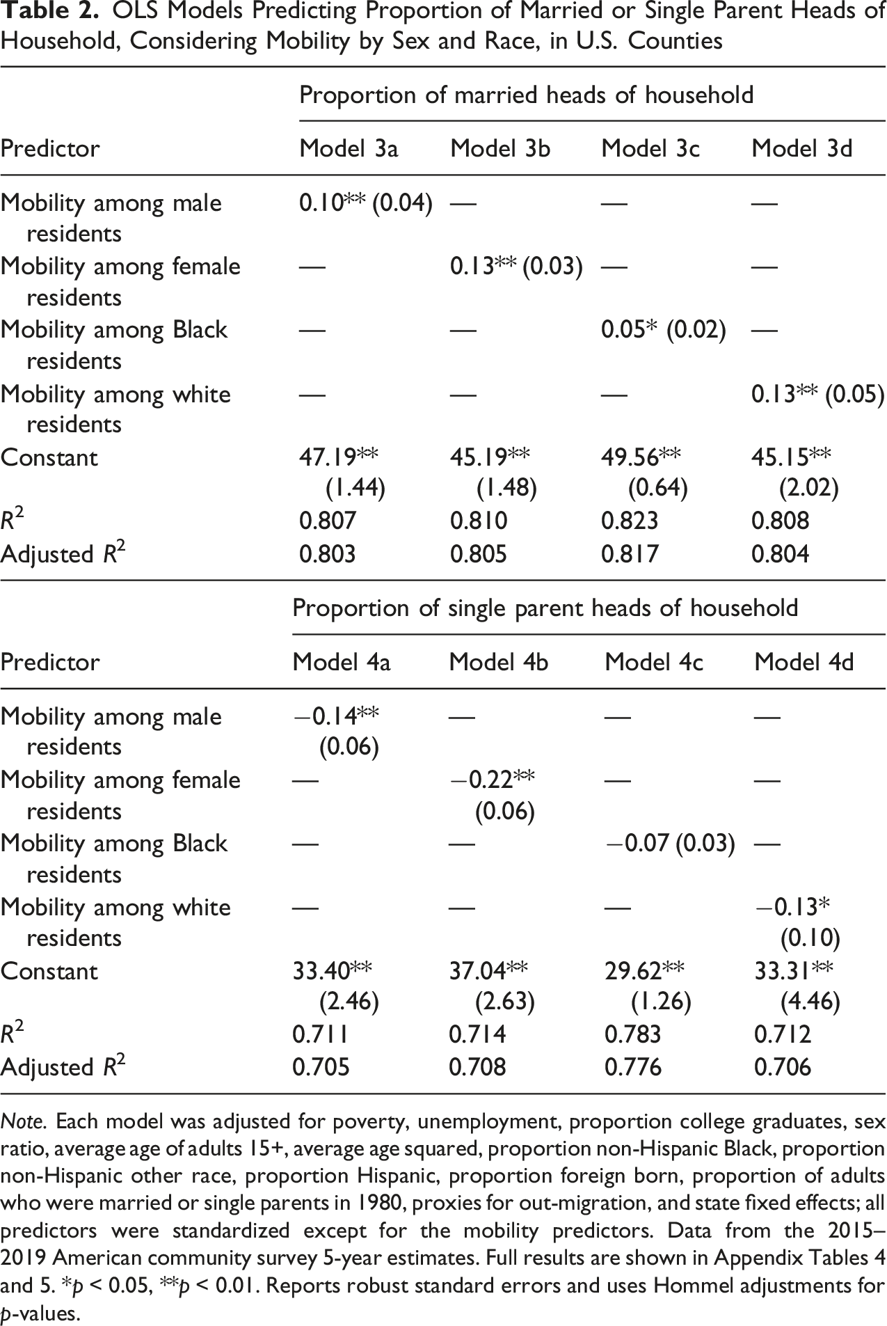
Note. Each model was adjusted for poverty, unemployment, proportion college graduates, sex ratio, average age of adults 15+, average age squared, proportion non-Hispanic Black, proportion non-Hispanic other race, proportion Hispanic, proportion foreign born, proportion of adults who were married or single parents in 1980, proxies for out-migration, and state fixed effects; all predictors were standardized except for the mobility predictors. Data from the 2015–2019 American community survey 5-year estimates. Full results are shown in Appendix Tables 4 and 5. *p < 0.05, **p < 0.01. Reports robust standard errors and uses Hommel adjustments for p-values.

Robustness Check: Intergenerational Mobility, Marriage, and Single Parenthood Among Specific Groups

Considering the associations between intergenerational mobility and subsequent marriage rate among individuals in specific age groups, key results from Models 5a and 5b are shown in Table 3 (full results in Appendix Table 5). The results of Model 5a are striking; the coefficient representing the association between intergenerational mobility and marriage rate among 30–39-year-olds (B = 0.49, p < 0.01) was nearly quadruple the coefficient from Model 1c (the corresponding model including all individuals ages 15 and over; B = 0.13, p < 0.01). This finding suggests that the rate at which young people raised in low-income households rise to the middle class is strongly associated with marriage rate among 30–39-year-olds. Additionally, it stands to reason that the effect sizes of the complementary age group—adults ages 40 and over—would be smaller than the effect sizes among 30–39-year-olds. Indeed, Model 5b suggests that the effect size of the association between intergenerational mobility and marriage was less than half as large for adults ages 40 and over (B = 0.20, p < 0.01) compared to adults ages 30–39.

Table 3.

OLS Models Predicting Proportion of Married Adults Among Specific Groups in U.S. Counties

	Proportion of married heads of household:
	(5a) Among adults ages 30–39	(5b) Among adults ages 40 and over	(6a) Among heads of household who have a high school diploma or less education	(6b) Among heads of households who have some college or more education
Mobility (Chetty-Hendren)	0.49** (0.08)	0.20** (0.04)	0.36** (0.05)	0.05 (0.05)
Constant	35.76** (3.45)	53.62** (1.60)	58.73** (1.98)	86.30** (2.00)
State fixed effects	Yes	Yes	Yes	Yes
Observations	3,115	3,115	3,115	3,115
R ²	0.603	0.694	0.798	0.390
Adjusted R²	0.594	0.687	0.794	0.377
Residual Std. Error	7.135 (df = 3049)	3.677 (df = 3049)	3.811 (df = 3049)	5.094 (df = 3049)
F statistic	71.106** (df = 65; 3049)	106.234** (df = 65; 3049)	185.182** (df = 65; 3049)	29.950** (df = 65; 3049)

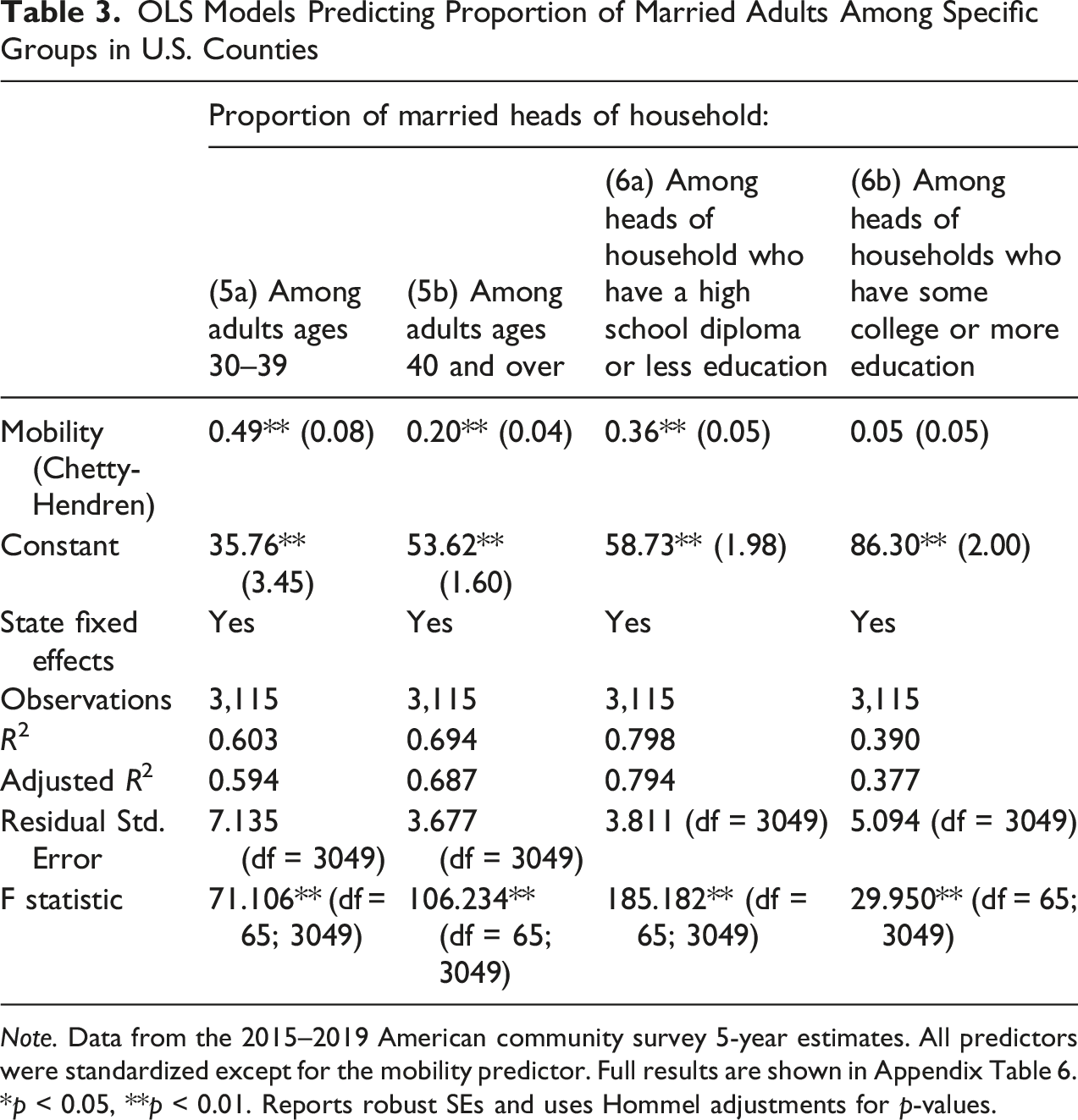
Note. Data from the 2015–2019 American community survey 5-year estimates. All predictors were standardized except for the mobility predictor. Full results are shown in Appendix Table 6. *p < 0.05, **p < 0.01. Reports robust SEs and uses Hommel adjustments for p-values.

Next, considering the associations between intergenerational mobility and marriage rates among individuals with differing educational attainment, key results from Models 6a and 6b are also shown in Table 3 (full results in Appendix Table 5). In Model 6a, we find that the association between intergenerational mobility and marriage among heads of household with a high school diploma or less education is significant (B = 0.36, p < 0.01). However, in Model 6b, considering only those heads of household with some college or more education, we find no significant relationship between intergenerational mobility and marriage, as we would expect.

Lastly, the results of Models 7a–7d confirm our hypothesis that households with somewhat lower incomes (below 185% FPL) would be more sensitive to the effects of intergenerational mobility on family formation outcomes compared to households with higher incomes (greater than or equal to 185% FPL); key results are shown in Table 4 (full results in Appendix Table 6). Considering the marriage rate, the effect size of the association between intergenerational mobility and marriage was more than three times larger among households with lower incomes (i.e., incomes below 185% FPL; Model 7a; B = 0.63, p < 0.01) compared to households with higher incomes (i.e., incomes greater than or equal to 185% FPL; Model 7b; B = 0.18, p < 0.01). Considering the rate of single parenthood, the effect size of the association between intergenerational mobility and single-parent households was also more than three times larger among households with lower incomes (Model 7c; B = −0.75, p < 0.01) compared to households with higher incomes (Model 7d; B = −0.19, p < 0.01).

Table 4.

OLS Models Predicting Proportion of Married or Single-Parent Heads of Household Among Specific Income Groups in U.S. Counties

	Proportion of married heads of household		Proportion of single-parent households
	(7a) Among households with incomes <185% FPL	(7b) Among households with incomes >=185% FPL	(7c) Among households with incomes <185% FPL	(7d) Among households with incomes >=185% FPL
Mobility (Chetty-Hendren)	0.63** (0.09)	0.18** (0.03)	−0.75** (0.08)	−0.19** (0.06)
Constant	26.41** (3.78)	78.95** (1.29)	87.71** (3.29)	25.12** (2.64)
State fixed effects	Yes	Yes	Yes	Yes
Observations	3,115	3,115	3,115	3,115
R ²	0.590	0.639	0.437	0.358
Adjusted R²	0.581	0.632	0.425	0.344
Residual Std. Error	7.313 (df = 3049)	3.087 (df = 3049)	9.569 (df = 3049)	5.597 (df = 3049)
F statistic	67.505** (df = 65; 3049)	83.114** (df = 65, 3049)	36.364** (df = 65; 3049)	26.110** (df = 65; 3049)

Discussion

The decline of marriage and the rise of single parenthood in the 20th and 21st centuries are broadly understood to be among the most consequential demographic shifts in the history of the United States. Quantitative social science has struggled to offer compelling explanations of the causes of these shifts, even while the evidence is clear that growing up with a single parent is associated with a host of deleterious outcomes (Ellwood & Jencks, 2004; McLanahan & Sandefur, 2009). At the same time, scholars are in near consensus that programs and policies seeking to promote marriage have also largely failed to deliver impacts on family formation, at least at this stage (Olivetti & Petrongolo, 2017; Randles, 2016)—although they may improve other outcomes, such as social poverty (Halpern-Meekin, 2020). This paper offers evidence that policies that increase intergenerational economic mobility at the community level should be a key policy goal. However, from a more holistic, societal perspective, acknowledging that many children in the US are being raised by single parents, we should also consider options that would mitigate the negative impacts of single parenthood through policy changes that socialize or otherwise reduce some of the largest costs of raising children, such as childcare (as is the case in most peer nations; Gornick et al., 2022a, 2022b; Hartley et al., 2022; Kwon, 2024).

This study offers empirical evidence that general economic conditions—beyond exogenous economic shocks—are significantly associated with family formation at the aggregate (county) level. Specifically, intergenerational mobility at the county level is positively associated with marriage rate in that county, all else equal. While a significant association between poverty and (in some models) unemployment and marriage remain, our findings suggest that intergenerational mobility is highly salient.

Results related to single parenthood also provide evidence in support of our initial hypothesis: that single parenthood will be less common in communities with relatively high intergenerational mobility. While consistent with literature on the 1970s coal boom in Appalachia, which showed that non-marital childbearing rates fell in the face of the boom (Black et al., 2013), our results are not consistent with an examination of more recent economic shocks to local economies (e.g., the fracking boom of the late 2000s), which showed that both marital and non-marital childbearing rates increased, but not marriage rates (Kearney & Wilson, 2018). Our results are, however, consistent with qualitative work conducted in the 2000s, which argued that, among lower income individuals, economic conditions matter less for childbearing than for marriage (Edin & Kefalas, 2011; Edin & Nelson, 2013; Edin & Reed, 2005; Gibson-Davis et al., 2005). In keeping with this, even in places with low rates of intergenerational mobility, rather than forgo childbearing, more parents are choosing to raise their children alone.

This paper builds on the work of Black et al. (2013), Kearney & Wilson (2018), Autor et al. (2019), and others in examining the strong regional patterns in economic factors, marriage, and single parenthood across the United States. It is worth noting that regional variation in rates of marriage and single parenthood no doubt reflect patterns in other domains—not just economic conditions. Counties with the lowest rates of marriage and highest rates of single parenthood, particularly in the South, also have some of the highest poverty rates (for which we adjusted in this analysis), some of the highest rates of low birthweight babies, and some of the shortest life expectancies in the nation. By contrast, counties in the upper Midwest, which have among the highest marriage and lowest single parenthood rates, have less poverty, fewer low birthweight babies, and longer lifespans than the nation as a whole (Edin et al., 2023, p. 5). These regional patterns are also similar to those seen in rates of “economic connectedness” across communities—the degree to which individuals of high and low socioeconomic standing interact, which can materially affect economic and labor market outcomes of young people with low socioeconomic status (Chetty et al., 2022).

This paper additionally builds on the work of Cherlin et al. (2016)—although we consider county-level intergenerational mobility and county-level family formation outcomes, rather than the relationship between county-level income inequality and individual-level family formation outcomes. Future research that utilizes the approach of Cherlin and colleagues (2016), matching individual-level outcomes with the county-level measure of intergenerational mobility that we utilize in this study, would further research in this area. Such work would permit the exploration of potential mechanisms linking intergenerational mobility within a community to individual marriage and childbearing behaviors.

To address potential concerns that selective migration out of a county may bias the association between intergenerational mobility and family formation outcomes within that county, we adjusted our analyses and robustness checks (where possible) for three proxies for out-migration. Even after doing so, the positive association between intergenerational mobility and marriage rate was robust, as was the negative association between intergenerational mobility and rate of single parenthood. Further, only one of the proxies for out-migration—the proportion of householders in a county who lived in the same house from 2018 to 2019—was consistently associated with both outcomes of interest. The limited evidence of significant associations between the other proxies for out-migration and the outcomes of interest suggests that out-migration does not negate the association between intergenerational mobility and family formation outcomes at the county level.

Our findings are robust to the inclusion of state fixed effects and various covariates known to be related to both marriage and single parenthood, yet this study is not without limitations. First, our findings are descriptive, not causal. While our findings do not directly lend evidence to the causes of the long-term retreat from marriage, they do offer evidence about the conditions in which we might expect marriage to become more common and single parenthood more rare. Second, it is possible that the associations between intergenerational mobility, marriage, and single parenthood that we report on are spurious, the result of other factors not captured in the models. Even so, it is worth noting that our effect sizes are substantively meaningful and our results are robust across a range of model specifications, including models that adjust for rates of marriage and single parenthood in 1980, before the Chetty-Hendren intergenerational mobility metric is captured. This leads us to cautiously reject the possibility that the relationships between mobility and subsequent marriage and single parenthood rates are merely a reflection of place-based differences in these outcomes over the long-term. Third, we encountered several limitations in working with data from the 1980 decennial census and the 2019 ACS. We were unable to construct lagged predictors of marriage and single parenthood rates for specific sociodemographic groups in 1980 and thus could not control for these lagged predictors in all robustness checks. We were also unable to construct rates of single parent households among householders of specific ages or educational attainment using the 2019 ACS data; several of our robustness checks were conducted only with alternate marriage rate outcomes for this reason. Despite these data limitations, our findings are robust across all models and all robustness checks.

Conclusion

Intergenerational mobility declined in the second half of the 20th century, during the same time period that marriage declined dramatically (Chetty et al., 2017; Davis & Mazumder, 2024). The relationship between these two important trends in American life deserves more study. If they are truly tied together, then reversing the trend in the long-term economic prospects of Americans should be a key policy goal. Our findings, viewed in conjunction with the prior literature, suggest that policies should expand economic opportunities for low-income Americans by helping to promote employment and education, boost earnings, and build wealth. These changes would promote not only economic wellbeing, but also child and family wellbeing.

Footnotes

ORCID iD

Michelle Sarah Livings

Ethical Considerations

Ethical approval was not required as the data underlying this article are all publicly available online.

Author Contributions

M.S. Livings: conceptualization; methodology; data curation; formal analysis; writing—original draft, review and editing; and visualization. K.J. Edin: conceptualization; methodology; writing—original draft, review and editing; and supervision. H.L. Shaefer: conceptualization; methodology; writing—original draft, review and editing; and supervision. S. Pachman: conceptualization; methodology; and writing—original draft, review and editing.

Funding

The authors received no financial support for the research, authorship, and/or publication of this article.

Declaration of Conflicting Interests

The authors declared no potential conflicts of interest with respect to the research, authorship, and/or publication of this article.

Data Availability Statement

The county-level measure of intergenerational mobility is available through the Opportunity Insights data repository (Opportunity Insights, 2026, https://opportunityinsights.org/data). All other measures are available through the U.S. Census Bureau website (U.S. Census Bureau, 2026, ).

Appendix

Table 1.

Summary Statistics, n = 3119 Counties (American Community Survey 2015–2019)

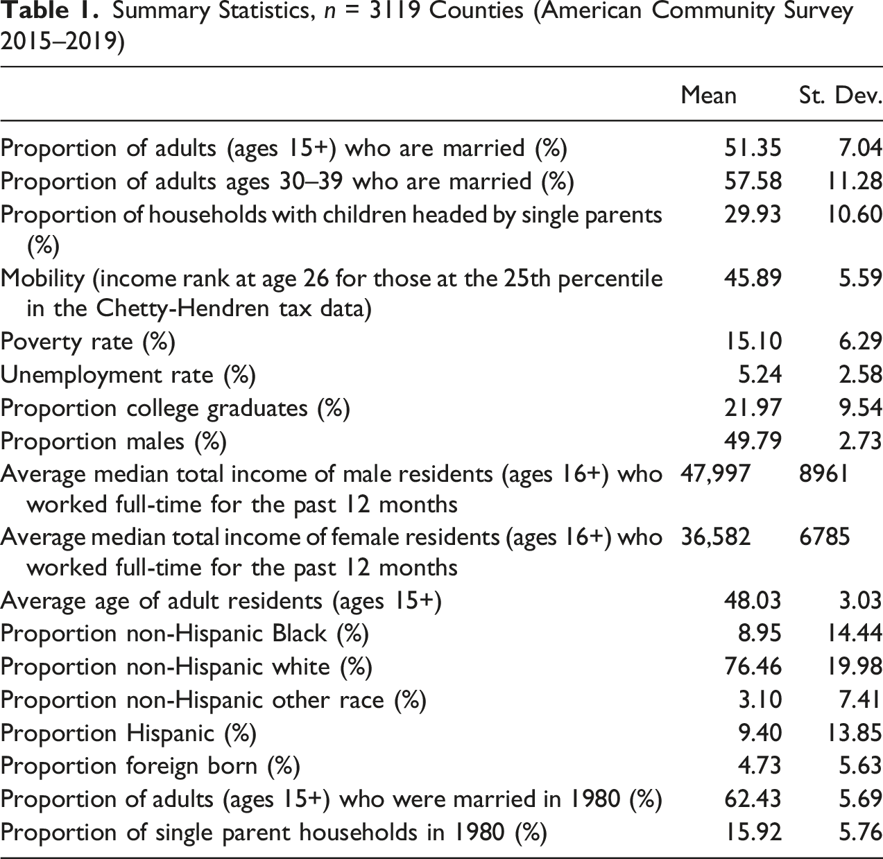
	Mean	St. Dev.
Proportion of adults (ages 15+) who are married (%)	51.35	7.04
Proportion of adults ages 30–39 who are married (%)	57.58	11.28
Proportion of households with children headed by single parents (%)	29.93	10.60
Mobility (income rank at age 26 for those at the 25th percentile in the Chetty-Hendren tax data)	45.89	5.59
Poverty rate (%)	15.10	6.29
Unemployment rate (%)	5.24	2.58
Proportion college graduates (%)	21.97	9.54
Proportion males (%)	49.79	2.73
Average median total income of male residents (ages 16+) who worked full-time for the past 12 months	47,997	8961
Average median total income of female residents (ages 16+) who worked full-time for the past 12 months	36,582	6785
Average age of adult residents (ages 15+)	48.03	3.03
Proportion non-Hispanic Black (%)	8.95	14.44
Proportion non-Hispanic white (%)	76.46	19.98
Proportion non-Hispanic other race (%)	3.10	7.41
Proportion Hispanic (%)	9.40	13.85
Proportion foreign born (%)	4.73	5.63
Proportion of adults (ages 15+) who were married in 1980 (%)	62.43	5.69
Proportion of single parent households in 1980 (%)	15.92	5.76

Appendix Table 2.

Correlation Matrix, n = 3119 Counties (American Community Survey 2015–2019)

		(1)	(2)	(3)	(4)	(5)	(6)	(7)	(8)	(9)	(10)	(11)	(12)	(13)	(14)	(15)	(16)
Proportion married in 2019	(1)	1.000
Single parent households in 2019	(2)	−0.715 p < 0.001	1.000
Mobility	(3)	0.639 p < 0.001	−0.621 p < 0.001	1.000
Poverty	(4)	−0.627 p < 0.001	0.658 p < 0.001	−0.491 p < 0.001	1.000
Unemployment	(5)	−0.543 p < 0.001	0.553 p < 0.001	−0.509 p < 0.001	0.641 p < 0.001	1.000
College graduates	(6)	0.053 p = 0.003	−0.278 p < 0.001	0.030 p = 0.090	−0.442 p < 0.001	−0.296 p < 0.001	1.000
Males	(7)	−0.052 p = 0.004	−0.130 p < 0.001	0.203 p < 0.001	−0.033 p = 0.065	−0.032 p = 0.073	−0.188 p < 0.001	1.000
Median income of employed males	(8)	0.270 p < 0.001	−0.385 p < 0.001	0.191 p < 0.001	−0.580 p < 0.001	−0.265 p < 0.001	0.625 p < 0.001	−0.069 p < 0.001	1.000
Median income of employed females	(9)	0.111 p < 0.001	−0.299 p < 0.001	0.054 p = 0.002	−0.528 p < 0.001	−0.232 p < 0.001	0.740 p < 0.001	−0.063 p < 0.001	0.791 p < 0.001	1.000
Average age of adults 15+	(10)	0.467 p < 0.001	−0.140 p < 0.001	0.317 p < 0.001	−0.193 p < 0.001	−0.164 p < 0.001	−0.244 p < 0.001	−0.084 p < 0.001	−0.143 p < 0.001	−0.189 p < 0.001	1.000
NH Black	(11)	−0.589 p < 0.001	0.630 p < 0.001	−0.589 p < 0.001	0.446 p < 0.001	0.399 p < 0.001	−0.098 p < 0.001	−0.126 p < 0.001	−0.181 p < 0.001	−0.137 p < 0.001	−0.212 p < 0.001	1.000
NH other race	(12)	−0.205 p < 0.001	0.118 p < 0.001	−0.094 p < 0.001	0.175 p < 0.001	0.252 p < 0.001	0.128 p < 0.001	0.020 p = 0.265	0.098 p < 0.001	0.186 p < 0.001	−0.210 p < 0.001	−0.088 p < 0.001	1.000
Hispanic	(13)	−0.121 p < 0.001	0.034 p = 0.056	−0.024 p = 0.176	0.076 p < 0.001	0.067 p < 0.001	−0.016 p = 0.371	0.145 p < 0.001	−0.039 p = 0.028	−0.032 p = 0.079	−0.270 p < 0.001	−0.117 p < 0.001	0.015 p = 0.411	1.000
Foreign born	(14)	−0.117 p < 0.001	−0.056 p = 0.002	−0.083 p < 0.001	−0.097 p < 0.001	−0.022 p = 0.225	0.368 p < 0.001	0.033 p = 0.068	0.250 p < 0.001	0.366 p < 0.001	−0.368 p < 0.001	−0.013 p = 0.460	0.151 p < 0.001	0.669 p < 0.001	1.000
Proportion married in 1980	(15)	0.719 p < 0.001	−0.463 p < 0.001	0.499 p < 0.001	−0.339 p < 0.001	−0.282 p < 0.001	−0.325 p < 0.001	0.049 p = 0.006	−0.015 p = 0.398	−0.191 p < 0.001	0.453 p < 0.001	−0.526 p < 0.001	−0.225 p < 0.001	0.030 p = 0.098	−0.173 p < 0.001	1.000
Single parent households in 1980	(16)	−0.750 p < 0.001	0.704 p < 0.001	−0.755 p < 0.001	0.528 p < 0.001	0.523 p < 0.001	0.048 p = 0.008	−0.165 p < 0.001	−0.156 p < 0.001	0.003 p < 0.875	−0.271 p < 0.001	0.722 p < 0.001	0.198 p < 0.001	0.046 p = 0.010	0.179 p < 0.001	−0.730 p < 0.001	1.000

Appendix Table 3.

OLS Models Predicting Proportion of Married Heads of Household, Considering Mobility by Sex and Race, in U.S. Counties

Predictor	Proportion of married heads of household
Predictor	Model 3a	Model 3b	Model 3c	Model 3d
Mobility among male residents	0.10** (0.04)	—	—	—
Mobility among female residents	—	0.13** (0.03)	—	—
Mobility among Black residents	—	—	0.05* (0.02)	—
Mobility among white residents	—	—	—	0.13** (0.05)
Poverty	−1.50** (0.15)	−1.48** (0.15)	−1.70** (0.16)	−1.49** (0.15)
Unemployment	−0.65** (0.12)	−0.65** (0.12)	−0.59** (0.13)	−0.64** (0.12)
Proportion college grads	−0.11 (0.18)	0.23 (0.18)	−0.22 (0.24)	−0.13 (0.18)
Sex ratio (proportion male)	−0.15 (0.13)	−0.21 (0.13)	0.05 (0.18)	−0.19 (0.13)
Median male income	1.15** (0.18)	1.16** (0.17)	1.07** (0.19)	1.15** (0.18)
Median female income	−0.33 (0.23)	−0.29 (0.22)	−0.18 (0.24)	−0.31 (0.23)
Average age of adults 15+	−6.32** (2.55)	−6.14** (2.54)	−5.60 (3.03)	−6.12** (2.56)
Average age squared	7.28** (2.46)	7.11** (2.44)	6.70** (2.97)	7.05** (2.46)
Proportion non-Hispanic Black	−1.53** (0.19)	−1.48** (0.18)	−1.74** (0.18)	−1.73** (0.17)
Proportion non-Hispanic other race^a	−0.49** (0.16)	−0.45** (0.16)	−0.48 (0.18)	−0.63** (0.17)
Proportion Hispanic	−0.76** (0.27)	−0.65** (0.28)	−0.64** (0.28)	−0.78** (0.25)
Proportion foreign born	0.58** (0.22)	0.53** (0.23)	0.37 (0.27)	0.55** (0.20)
Proportion adults (ages 15+) married in 1980	2.25** (0.23)	2.21** (0.23)	2.05** (0.24)	2.28** (0.23)
Population change from 2018 to 2019	−0.06 (0.05)	−0.07 (0.05)	−0.05 (0.04)	−0.04 (0.05)
Proportion living in same home from 2018 to 2019	1.15** (0.14)	1.13** (0.15)	1.18** (0.17)	1.11** (0.15)
Median number of years living in current house	−0.23 (0.17)	−0.29 (0.17)	−0.31 (0.17)	−0.25 (0.17)
Constant	47.19** (1.44)	45.19** (1.48)	49.56** (0.64)	45.15** (2.02)
State fixed-effects	Yes	Yes	Yes	Yes
Observations	3,108	3,105	1,911	3,111
R ²	0.807	0.810	0.823	0.808
Adjusted R²	0.803	0.805	0.817	0.804
Residual Std. Error	3.114 (df = 3041)	3.089 (df = 3038)	2.709 (df = 1844)	3.110 (df = 3044)
F statistic	192.799** (df = 66; 3041)	195.749** (df = 66; 3038)	130.026** (df = 66; 1844)	193.721** (df = 66; 3044)

Note. Data from the 2015–2019 American community survey 5-year estimates. All predictors were standardized except for the mobility predictors. *p < .05 **p < 0.01 Reports robust SEs and uses Hommel adjustments for p-values.

^a“Other race” includes non-Hispanic Asian, non-Hispanic American Indian/Alaska Native, and non-Hispanic Native Hawaiian or Pacific Islander.

Appendix Table 4.

OLS Models Predicting Proportion of Single-Parent Heads of Household, Considering Mobility by Sex and Race, in U.S. Counties

Predictor	Proportion of single-parent households
Predictor	Model 4a	Model 4b	Model 4c	Model 4d
Mobility among male residents	−0.14** (0.06)	—	—	—
Mobility among female residents	—	−0.22** (0.06)	—	—
Mobility among Black residents	—	—	−0.07 (0.03)	—
Mobility among white residents	—	—	—	−0.13* (0.10)
Poverty	2.83** (0.39)	2.82** (0.38)	3.20** (0.49)	2.75** (0.38)
Unemployment	0.32 (0.31)	0.30 (0.30)	0.20 (0.49)	0.32 (0.30)
Proportion college grads	−0.67 (0.37)	−0.57 (0.36)	−0.85* (0.40)	−0.64 (0.35)
Sex ratio (proportion male)	−0.71** (0.27)	−0.70** (0.27)	−1.07** (0.23)	−0.69** (0.27)
Median male income	−0.47 (0.20)	−0.54 (0.21)	−0.59 (0.31)	−0.54 (0.20)
Median female income	−0.69 (0.35)	−0.63 (0.38)	−0.74 (0.44)	−0.65 (0.35)
Average age of adults 15+	16.34** (3.56)	15.82** (3.53)	19.05** (3.56)	15.76** (3.55)
Average age squared	−14.84** (3.57)	−14.31** (3.55)	−17.30** (3.63)	−14.32** (3.57)
Proportion non-Hispanic Black	3.62** (0.35)	3.59** (0.34)	4.24** (0.36)	3.86** (0.38)
Proportion non-Hispanic other race^a	1.16** (0.27)	1.09** (0.27)	1.11** (0.22)	1.33** (0.29)
Proportion Hispanic	2.70** (0.40)	2.52** (0.42)	2.43** (0.34)	2.72** (0.37)
Proportion foreign born	−1.71** (0.33)	−1.60** (0.33)	−1.25** (0.43)	−1.79** (0.36)
Proportion single-parent households in 1980	2.84** (0.36)	2.71** (0.38)	2.11** (0.37)	2.98** (0.36)
Population change from 2018 to 2019	0.07 (0.10)	0.08 (0.10)	0.18 (0.11)	0.07 (0.10)
Proportion living in same home from 2018 to 2019	−0.70** (0.22)	−0.67** (0.23)	−1.10** (0.23)	−0.64* (0.22)
Median number of years living in current house	−0.96** (0.33)	−0.90** (0.33)	−1.05** (0.42)	−0.98** (0.34)
Constant	33.40** (2.46)	37.04** (2.63)	29.62** (1.26)	33.31** (4.46)
State fixed-effects	Yes	Yes	Yes	Yes
Observations	3,108	3,105	1,911	3,111
R ²	0.71	0.714	0.783	0.712
Adjusted R²	0.705	0.708	0.776	0.706
Residual Std. Error	5.736 (df = 3041)	5.703 (df = 3038)	4.857 (df = 1844)	5.731 (df = 3044)
F statistic	113.603** (df = 66; 3041)	115.077** (df = 66, 3038)	101.003** (df = 66; 1844)	113.961** (df = 66, 3044)

Note. Data from the 2015–2019 American Community Survey 5-year estimates. All predictors were standardized except for the mobility predictors. *p < .05, **p < 0.01 Reports robust SEs and uses Hommel adjustments for p-values.

^a“Other race” includes non-Hispanic Asian, non-Hispanic American Indian/Alaska Native, and non-Hispanic Native Hawaiian or Pacific Islander.

Appendix Table 5.

OLS Models Predicting Proportion of Married Heads of Household Among Specific Groups in U.S. Counties

Predictor:	Proportion of married heads of household:
Predictor:	(5a) Among adults ages 30–39	(5b) Among adults ages 40 and over	(6a) Among heads of household who have a high school diploma or less education	(6b) Among heads of households who have some college or more education
Mobility (Chetty-Hendren)	0.49** (0.08)	0.20** (0.04)	0.36** (0.05)	0.05 (0.05)
Poverty	−1.90** (0.35)	−2.01** (0.24)	−2.40** (0.23)	−0.75** (0.29)
Unemployment	−0.84** (0.19)	−0.54** (0.13)	−0.59** (0.12)	−0.73** (0.16)
Proportion college grads	−1.10** (0.53)	0.33 (0.18)	−0.62** (0.24)	0.82** (0.26)
Sex ratio (proportion male)	−2.00** (0.36)	−0.27 (0.17)	0.94** (0.21)	0.57** (0.13)
Median male income	1.89** (0.45)	1.22** (0.20)	0.19 (0.14)	0.76** (0.25)
Median female income	−0.20 (0.36)	−0.65** (0.26)	−0.32 (0.22)	−0.99** (0.31)
Average age of adults 15+	−15.14** (4.74)	−10.89** (2.62)	−15.40** (2.31)	−4.84 (1.79)
Average age of adults, squared	13.18** (4.87)	9.94** (2.56)	15.65** (2.28)	5.87 (1.73)
Proportion non-Hispanic Black	−4.05** (0.29)	−2.66** (0.19)	−3.76** (0.19)	−2.28** (0.12)
Proportion non-Hispanic other race^a	−1.49** (0.33)	−0.62** (0.18)	−1.51** (0.13)	−0.98** (0.23)
Proportion Hispanic	−1.91** (0.67)	−0.63** (0.36)	−1.99** (0.28)	−0.65 (0.19)
Proportion foreign born	0.88* (0.45)	0.42 (0.30)	0.54** (0.28)	0.45 (0.23)
Population change from 2018 to 2019	−0.15 (0.14)	−0.08 (0.08)	−0.07 (0.07)	−0.05 (0.07)
Proportion living in same home from 2018 to 2019	1.53** (0.37)	1.30** (0.17)	0.67** (0.20)	−0.16 (0.20)
Median number of years living in current house	−0.79* (0.40)	0.30 (0.20)	0.81** (0.18)	0.46 (0.32)
Constant	35.76** (3.45)	53.62** (1.60)	58.73** (1.98)	86.30** (2.00)
State fixed-effects	Yes	Yes	Yes	Yes
Observations	3,115	3,115	3,115	3,115
R ²	0.603	0.694	0.798	0.390
Adjusted R²	0.594	0.687	0.794	0.377
Residual Std. Error	7.135 (df = 3049)	3.677 (df = 3049)	3.811 (df = 3049)	5.094 (df = 3049)
F statistic	71.106** (df = 65; 3049)	106.234** (df = 65; 3049)	185.182** (df = 65; 3049)	29.950** (df = 65; 3049)

Note. Data from the 2015–2019 American community survey 5-year estimates. All predictors were standardized except for the mobility predictor. *p < .05, **p < 0.01 Reports robust SEs and uses Hommel adjustments for p-values.

^a“Other race” includes non-Hispanic Asian, non-Hispanic American Indian/Alaska Native, and non-Hispanic native Hawaiian or Pacific Islander.

Appendix Table 6.

OLS Models Predicting Proportion of Married or Single-Parent Heads of Household Among Specific Income Groups in U.S. Counties

Predictor	Proportion of married heads of household:		Proportion of single-parent households
Predictor	(7a) Among households with incomes <185% FPL	(7b) Among households with incomes ≥185% FPL	(7c) Among households with incomes <185% FPL	(7d) Among households with incomes ≥185% FPL
Mobility (Chetty-Hendren)	0.63** (0.09)	0.18** (0.03)	−0.75** (0.08)	−0.19** (0.06)
Poverty	−1.01** (0.35)	0.00 (0.15)	1.26** (0.49)	−0.37 (0.18)
Unemployment	−0.35 (0.27)	−0.45** (0.11)	0.26 (0.35)	0.74** (0.23)
Proportion college grads	−0.90* (0.38)	0.99** (0.18)	1.73** (0.47)	−0.47 (0.27)
Sex ratio (proportion males)	1.25** (0.35)	0.69** (0.12)	−0.83* (0.38)	−0.68** (0.20)
Median male income	−1.43** (0.27)	0.56** (0.13)	2.64** (0.48)	−1.47** (0.28)
Median female income	0.34 (0.38)	−0.81** (0.21)	−1.58** (0.50)	0.66 (0.36)
Average age of adults 15+	−33.65** (4.49)	−4.56** (1.61)	27.76** (5.13)	6.91* (2.18)
Average age of adults, squared	34.14** (4.41)	5.31** (1.61)	−26.02** (5.10)	−6.70 (2.26)
Proportion non-Hispanic Black	−4.46** (0.34)	−2.35** (0.12)	4.57** (0.40)	2.49** (0.24)
Proportion non-Hispanic other race	−1.54** (0.23)	−1.13** (0.14)	1.08** (0.30)	1.68** (0.19)
Proportion Hispanic	−2.88** (0.38)	−1.10** (0.16)	3.02** (0.67)	1.58** (0.58)
Proportion foreign born	3.04** (0.35)	0.15 (0.18)	−4.11** (0.49)	−1.00** (0.53)
Population change from 2018 to 2019	0.01 (0.09)	−0.06 (0.06)	−0.05 (0.13)	0.00 (0.07)
Proportion living in same home from 2018 to 2019	1.57** (0.28)	0.13 (0.16)	−1.85** (0.25)	−0.23 (0.23)
Median number of years living in current house	1.31** (0.32)	0.39** (0.15)	−0.93 (0.52)	−0.81** (0.29)
Constant	26.41** (3.78)	78.95** (1.29)	87.71** (3.29)	25.12** (2.64)
State fixed-effects	Yes	Yes	Yes	Yes
Observations	3,115	3,115	3,115	3,115
R ²	0.590	0.639	0.437	0.358
Adjusted R²	0.581	0.632	0.425	0.344
Residual Std. Error	7.313 (df = 3049)	3.087 (df = 3049)	9.569 (df = 3049)	5.597 (df = 3049)
F statistic	67.505** (df = 65; 3049)	83.114** (df = 65, 3049)	36.364** (df = 65; 3049)	26.110** (df = 65; 3049)

^a“Other race” includes non-Hispanic Asian, non-Hispanic American Indian/Alaska Native, and non-Hispanic Native Hawaiian or Pacific Islander.

References

Aaronson

Mazumder

(2008). Intergenerational economic mobility in the United States, 1940 to 2000. Journal of Human Resources, 43(1), 139–172. https://doi.org/10.3368/jhr.43.1.139

Autor

Dorn

Hanson

(2019). When work disappears: Manufacturing decline and the falling marriage market value of young men. American Economic Review: Insights, 1(2), 161–178. https://doi.org/10.1257/aeri.20180010

Bell

M. C.

Edin

Wood

H. M.

Mondé

G. C.

(2018). Relationship repertoires, the price of parenthood, and the costs of contraception. Social Service Review, 92(3), 313–348. https://doi.org/10.1086/699159

Black

D. A.

Kolesnikova

Sanders

S. G.

Taylor

L. J.

(2013). Are children “normal”. The Review of Economics and Statistics, 95(1), 21–33. https://doi.org/10.1162/REST_a_00257

Cherlin

A. J.

Ribar

D. C.

Yasutake

(2016). Nonmarital first births, marriage, and income inequality. American Sociological Review, 81(4), 749–770. https://doi.org/10.1177/0003122416653112

Chetty

Grusky

Hell

Hendren

Manduca

Narang

(2017). The fading American dream: Trends in absolute income mobility since 1940. Science, 356(6336), 398–406. https://doi.org/10.1126/science.aal4617

Chetty

Hendren

(2018). The impacts of neighborhoods on intergenerational mobility II: County-level estimates. The Quarterly Journal of Economics, 133(3), 1163–1228. https://doi.org/10.1093/qje/qjy006

Chetty

Hendren

Kline

Saez

(2014). Where is the land of opportunity? The geography of intergenerational mobility in the United States. The Quarterly Journal of Economics, 129(4), 1553–1623. https://doi.org/10.1093/qje/qju022

Chetty

Jackson

M. O.

Kuchler

Stroebel

Hendren

Fluegge

R. B.

Gong

Gonzalez

Grondin

Jacob

Johnston

Koenen

Laguna-Muggenburg

Mudekereza

Rutter

Thor

Townsend

Zhang

Bailey

Wernerfelt

(2022). Social capital I: Measurement and associations with economic mobility. Nature, 608(7921), 108–121. https://doi.org/10.1038/s41586-022-04996-4

10.

Connolly

Haeck

(2024). Differences across place in intergenerational income mobility. In Research handbook on intergenerational inequality (pp. 178–191). Edward Elgar Publishing, Inc. https://www.elgaronline.com/edcollchap/book/9781800888265/book-part-9781800888265-22.xml

11.

Cross

C. J.

(2020). Racial/ethnic differences in the association between family structure and children’s education. Journal of Marriage and Family, 82(2), 691–712. https://doi.org/10.1111/jomf.12625

12.

Davis

J. M. V.

Mazumder

(2024). The decline in intergenerational mobility after 1980. The Review of Economics and Statistics, 108(1), 1–47. https://doi.org/10.1162/rest_a_01413

13.

Edin

K. J.

Kefalas

M. J.

(2011). Promises I can keep: Why low-income women put motherhood before marriage (Revised ed.). University of California Press.

14.

Edin

K. J.

Nelson

T. J.

(2013). Doing the best I can: Fatherhood in the inner city. University of California Press.

15.

Edin

K. J.

Reed

J. M.

(2005). Why don’t they just get married? Barriers to marriage among the disadvantaged. The Future of Children, 15(2), 117–137. https://doi.org/10.1353/foc.2005.0017

16.

Edin

K. J.

Shaefer

H. L.

Nelson

T. J.

(2023). The injustice of place: Uncovering the legacy of poverty in America. Mariner Books.

17.

Ellwood

D. T.

Jencks

(2004). The spread of single-parent families in the United States since 1960. KSG Working Paper No. RWP04-008. https://doi.org/10.2139/ssrn.517662

18.

Federal Interagency Forum on Child and Family Statistics . (2023). America’s children: Key national indicators of well-being, 2023. Federal Interagency Forum on Child and Family Statistics. https://www.childstats.gov/americaschildren/

19.

Gibson-Davis

C. M.

Edin

McLanahan

(2005). High hopes but even higher expectations: The retreat from marriage among low-income couples. Journal of Marriage and Family, 67(5), 1301–1312. https://doi.org/10.1111/j.1741-3737.2005.00218.x

20.

Gibson-Davis

C. M.

Gassman-Pines

Lehrman

(2018). “His” and “Hers”: Meeting the economic bar to marriage. Demography, 55(6), 2321–2343. https://doi.org/10.1007/s13524-018-0726-z

21.

Gornick

J. C.

Maldonado

L. C.

Sheely

(2022a). Effective policies for single-parent families and prospects for policy reforms in the United States: Concluding reflections. The ANNALS of the American Academy of Political and Social Science, 702(1), 236–251. https://doi.org/10.1177/00027162221133682

22.

Gornick

J. C.

Maldonado

L. C.

Sheely

(2022b). Single-parent families and public policy in high-income countries: Introduction to the volume. The ANNALS of the American Academy of Political and Social Science, 702(1), 8–18. https://doi.org/10.1177/00027162221133250

23.

Halpern-Meekin

(2020). Social poverty and relational resources. Contexts, 19(2), 40–45. https://doi.org/10.1177/1536504220920195

24.

Hartley

R. P.

Mattingly

M. J.

Waldfogel

Wimer

(2022). Paying for childcare to work? Evaluating the role of policy in affordable care and child poverty. Social Service Review, 96(1), 34–72. https://doi.org/10.1086/718635

25.

Hommel

(1988). A stagewise rejective multiple test procedure based on a modified bonferroni test. Biometrika, 75(2), 383–386. https://doi.org/10.2307/2336190

26.

Ishizuka

(2018). The economic foundations of cohabiting couples’ union transitions. Demography, 55(2), 535–557. https://doi.org/10.1007/s13524-018-0651-1

27.

Jácome

Kuziemko

Naidu

(2021). Mobility for all: Representative intergenerational mobility estimates over the 20th century. NBER Working Paper Series, 29289, 302. https://ideas.repec.org//p/pri/cepsud/302.html

28.

Kearney

M. S.

Wilson

(2018). Male earnings, marriageable men, and nonmarital fertility: Evidence from the fracking boom. The Review of Economics and Statistics, 100(4), 678–690. https://doi.org/10.1162/rest_a_00739

29.

Kwon

S. J.

(2024). The effects of the child and dependent care tax credit (CDCTC) on child-care use and maternal labor supply. Social Service Review, 98(2), 293–328. https://doi.org/10.1086/730124

30.

Lichter

D. T.

Price

J. P.

Swigert

J. M.

(2020). Mismatches in the marriage market. Journal of Marriage and Family, 82(2), 796–809. https://doi.org/10.1111/jomf.12603

31.

Livingston

(2018, April 25). The changing profile of unmarried parents. Pew Research Center. https://www.pewresearch.org/social-trends/2018/04/25/the-changing-profile-of-unmarried-parents/

32.

Lopoo

L. M.

Carlson

M. J.

(2008). Marriageability among the partners of young mothers. Social Service Review, 82(2), 253–271. https://doi.org/10.1086/589902

33.

Mann

Edin

K. J.

Shaefer

H. L.

(2024). Understanding the relationship between intergenerational mobility and community violence. Proceedings of the National Academy of Sciences, 121(33), Article e2309066121. https://doi.org/10.1073/pnas.2309066121

34.

McLanahan

Sandefur

G. D.

(2009). Growing up with a single parent: What hurts, what helps. Harvard University Press.

35.

Olivetti

Petrongolo

(2017). The economic consequences of family policies: Lessons from a century of legislation in high-income countries. Journal of Economic Perspectives, 31(1), 205–230. https://doi.org/10.1257/jep.31.1.205

36.

Parker

Stepler

(2017, September 14). As U.S. marriage rate hovers at 50%, education gap in marital status widens. Policy Commons. https://policycommons.net/artifacts/617670/as-us/1598523/

37.

Randles

(2016). Proposing prosperity? Marriage education policy and inequality in America. Columbia University Press. https://doi.org/10.7312/rand17030

38.

Tolnay

Beck

E. M.

(1995). A festival of violence: An analysis of southern lynchings, 1882-1930. University of Illinois Press. https://www.press.uillinois.edu/books/?id=p064135

39.

U.S. Census Bureau . (2024). American community survey (ACS). Census.Gov. https://www.census.gov/programs-surveys/acs

40.

Waller

M. R.

McLanahan

S. S.

(2005). “His” and “her” marriage expectations: Determinants and consequences. Journal of Marriage and Family, 67(1), 53–67. https://doi.org/10.1111/j.0022-2445.2005.00005.x

41.

Watson

McLanahan

(2011). Marriage meets the Joneses: Relative income, identity, and marital status. The Journal of Human Resources, 46(3), 482–517. https://doi.org/10.3368/jhr.46.3.482

42.

Wilson

W. J.

(1987). The truly disadvantaged: The inner city, the underclass, and public policy (2nd ed.). University of Chicago Press.

43.

Wilson

W. J.

Neckerman

K. M.

(1987). Poverty and family structure: The widening gap between evidence and public policy issues. In Fighting poverty: What works and what doesn’t (pp. 232–259). Harvard University Press.