Evidence-Based Medicine in Otolaryngology,Part 3: Everyday Probabilities

Everyday Statistics: Predictive Values of Binary Diagnostic Tests

Understanding the predictive probabilities associated with diagnostic testing allows us to convey accurate information to patients, a key aspect of evidence-based practice. It is a critical skill, ideally based on some familiarity with conditional probabilities. This skill is frequently needed in common clinical scenarios, such as the following:

Answer 1: A, 23%. The most common numerical error made by physicians is inaccurate determination of the predictive value of a diagnostic test. ¹ When physicians are tested with a clinical scenario like the one above, only 3% to 22% can identify the correct predicted probability of disease.^2-8 In general, most physicians will overestimate the probability of true disease.^1,8 As many as 78% to 95% of physicians will make this specific error.^3,8

As otolaryngologists, our daily routines are ensconced in numbers. Some are certainties, such as measured weights and heights or established medication doses. Others, like many aspects of medicine, are uncertainties, such as whether a specific individual patient with malignancy will be alive in 5 years or whether a specific individual will have a future perioperative complication. Insidious and ubiquitous, probabilities are present whenever we consider diagnostic tests, management of disease, or risks of interventions.

One of the key obstacles to evidence-based practice is physician innumeracy. Such innumeracy additionally creates the potential to convey inaccurate information to patients, even with the best of intentions. Multiple publications have described the statistics needed to understand published data from clinical studies. Those statistics are crucial when considering the efficacy of interventions in clinical studies, and we espouse learning those concepts well. Additional statistics are, however, omnipresent in everyday clinical life, even for those of us who do not participate in research or academic projects. Understanding these concepts is a cornerstone of evidence-based practice. Therefore, the next installments in this series focus on statistics relevant to our daily practices. This installment will focus on probabilities associated with diagnostic tests with binary results, that is, those with only positive or negative results. The subsequent installment will focus on the probabilities associated with diagnostic test results with multilevel or continuous results.

Diagnostic Tests

Ideally, diagnostic test results have strong validity, meaning they are true measures of the disease state in question. The validity of diagnostic tests is typically described in terms of their sensitivity and specificity. These descriptions are useful in that they measure the properties of the test itself, irrespective of the patient population in which it is utilized. Understanding the properties of the test itself can be very useful when planning a screening program for a large population or when comparing options for diagnostic tests. In day-to-day clinical practice, however, the key question is not about the test, but about the patient. The crucial question is, “If this test is positive, then does my patient have disease?” While sensitivity and specificity are useful, they alone are not sufficient to answer this clinical question. They cannot independently estimate the probability of disease in a particular patient, given a particular test result. Therefore, we will describe them briefly, but we spend the bulk of this discussion on Bayes theorem and the conditional probabilities that determine positive and negative predictive values of diagnostic tests.

Sensitivity and Specificity of Diagnostic Tests

Diagnostics tests with binary results yield positive or negative results, which can be true positives, false positives, true negatives, or false negatives ( Figure 1 ). The sensitivity of a test for a given disease is defined as the proportion of patients who truly have a disease that tests positive for that disease. If the sensitivity for the test is high, then the risk of false negatives is low. To better understand this relationship, consider how sensitivity is calculated: sensitivity = true positives / (true positives + false negatives). If the number of false negatives is 0, sensitivity is 100%. A negative result is therefore more valid (ie, a negative result is more likely to represent true lack of disease) when a test has high sensitivity. For example, if the sensitivity of a test is 95%, then the risk of false negatives is quite low at 5%, which suggests that a negative test is very likely to represent a true lack of disease.

OPEN IN VIEWER

Figure 1.

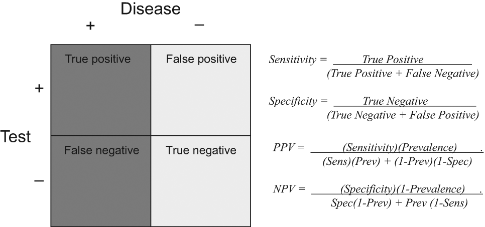
Calculations for sensitivity, specificity, positive predictive value (PPV), and negative predictive value (NPV) in tests with binary results.

The specificity of a test for a disease is defined as the proportion of patients who truly are disease free that tests negative for that disease. A high specificity means that the false positive rate is low. To better understand this meaning, consider how specificity is calculated: specificity = true negatives / (true negatives + false positives). Thus, if the number of false positives is 0, then specificity is 100%. A positive result is thus more meaningful when a test has high specificity. If the specificity of a test is estimated at 97%, then there is a 3% risk of false positives, which suggests that a positive result is very likely to represent the presence of true disease.

Both sensitivity and specificity are conditional probabilities where one conditions on the presence of disease or the absence of disease, respectively. Conditional probabilities describe the chance of an event occurring, given that another event has already occurred. Sensitivity describes the probability of a positive test result among those who truly have disease. Specificity describes the probability of a negative test result among those who actually have no disease. While these probabilities are conditional on disease presence or absence, they are not conditional on patient characteristics. Whether the test is performed on the first or last patient of the day, its inherent sensitivity and specificity will remain the same.

These metrics, however, provide no immediate answers when that first or last patient asks, “Given that my test was positive, what is the probability that I actually have cancer?” Since sensitivity is defined on the basis of only people who truly have disease, it can only describe a population in which everyone has disease. Likewise, since specificity is defined on the basis of only people who actually are without disease, it can only describe a population in which everyone is disease free ( Figure 2 ). The presence or absence of the disease in a given patient in the office is an unknown—it is unclear whether she truly has the disease or not (otherwise, you would not be ordering a diagnostic test!). Therefore, this uncertainty cannot be described solely in terms that describe a population that is purely diseased or purely disease free. The patient in the office is best described in terms of a population that contains both diseased and disease-free patients ( Figure 3 ).

OPEN IN VIEWER

Figure 2.

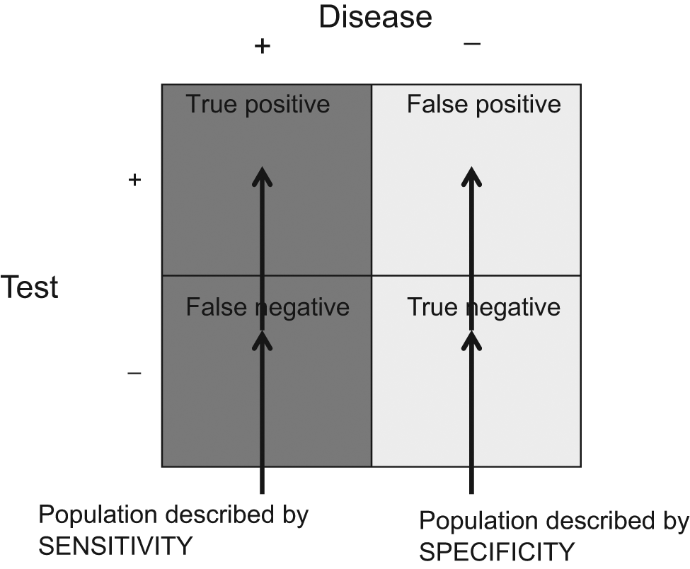
Populations described by sensitivity (all with disease) and specificity (all without disease). Sensitivity and specificity are defined in populations that are either purely diseased (dark gray) or purely disease free (light gray).

OPEN IN VIEWER

Figure 3.

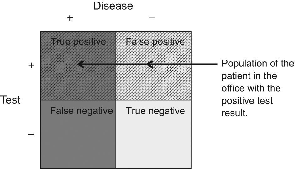
The population of patients with a positive test result is mixed; it contains those with true disease as well as those without true disease.

Predictive Values of Diagnostic Tests

The key point of interest in each patient encounter is the predictive value of the diagnostic test result for that patient; that is, given that the test was positive in this patient, what is the probability that this patient has true malignancy? This question defines the positive predictive value (PPV), a probability defined in a population of mixed disease status. The predictive value of a diagnostic test in such a mixed population depends on the prevalence of the disease and on the inherent properties of the test. The prevalence of the disease dictates the overall risk of disease in that underlying mixed population. That overall risk is then more specifically defined based on the presence of a positive test result.

Therefore, predictive values are conditional probabilities, where one conditions on the test result (not the presence or absence of disease). Such conditional probabilities can be calculated according to Bayes theorem. Bayes theorem can be expressed in several ways. The most widely used definition can be conveyed in terms of 2 events, A and B. The conditional probability of event A given that event B has occurred is given by the joint probability of events A and B divided by the unconditional probability of event B. Expressed in mathematic terms, this is Pr(A|B) = Pr(A, B)/Pr(B). In English, this means that the predictive value of the test is calculated from the prevalence of disease, the intrinsic characteristics of the test, and the probability of the test result. Mathematically, this means the probability that disease is present given that the test is positive (PPV) is equal to the probability of a positive test given that the disease is present, multiplied by the prevalence of disease, divided by the probability of a positive test ( Figure 4 ). These Bayesian calculations may seem like a mouthful, but they can be calculated in a straightforward way. If test results are binary, they can be calculated from the sensitivity, specificity, and prevalence of disease ( Figure 1 , Figure 4 ). In addition, predictive values vary according to expected rules, making them less complicated than they may initially seem. Positive predictive value will increase if prevalence increases, sensitivity increases, and the overall probability of a positive result decreases.

OPEN IN VIEWER

Figure 4.

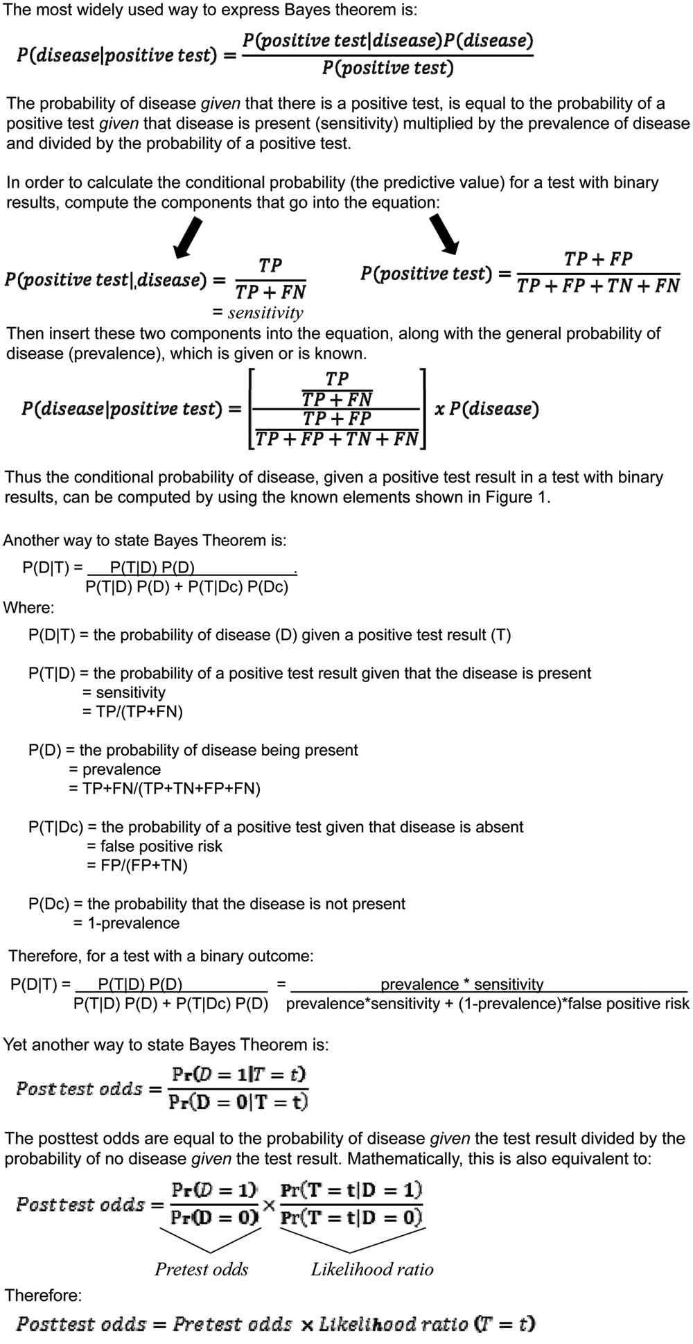
Calculation of positive and negative predictive values according to Bayes theorem.

Likelihood Ratios

Likelihood ratios (LRs) are another way to determine the probability of disease in a specific patient, given a known test result. The LR for a given test result is simply defined as the ratio of the probability of the test result in patients with the disease to the probability of the test result in patients without the disease ( Figure 5 ). Like the sensitivity and specificity, the LR is a property of the diagnostic test itself. In fact, for binary test results, one can mathematically simplify the LR to simple equations defined in terms of the sensitivity and specificity. The LR for a positive test result (LR+) is the ratio of the sensitivity to the false positive fraction. The LR for a negative test result (LR−) is the ratio of the false negative fraction to the specificity. For example, if both sensitivity and specificity are estimated at 85%, the LR if the test result is positive (LR+) is 5.7. The LR if the test result is negative (LR−) is 0.2. Like sensitivity and specificity, however, the LR is not enough alone to determine the probability of disease in the patient sitting in the office.

OPEN IN VIEWER

Figure 5.

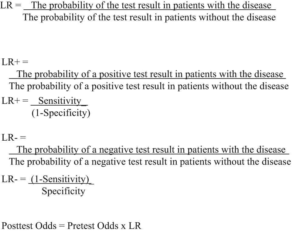
Likelihood ratios (LRs). Formulas are shown for the LR for a positive test result (LR+) and the LR for a negative test result (LR–).

Pretest odds are needed to use the LR to determine the posttest potential for true disease in that patient. Pretest odds quantify the expected potential for disease, given known patient features prior to the diagnostic test. Pretest odds describe the same state as pretest probability but quantify it in a different way. For example, in patients who have been irradiated, the pretest probability of malignancy is 30%. This probability has been calculated from numbers that suggest that 3 out of 10 irradiated patients with thyroid nodules have malignancy; that is, pretest probability = 3/10 = 0.3 = 30%. That same risk can also be described in terms of odds, which is the probability that an event will occur divided by the probability that it will not occur. Odds describe the chance that the event will happen compared with it not happening. In this case, pretest odds = 0.3/(1 – 0.3) = 0.3/0.7 = 0.43. This is the patient in your office asking, “Doc, how much more likely is it that I have cancer rather than no cancer?”

Multiplying the pretest odds by the LR gives the posttest odds of disease. The posttest odds define the odds of true disease, given the diagnostic test finding and the pretest patient characteristics. For example, in the scenario with the irradiated patient, the posttest odds with a positive test result are 2.45 (0.43 × 5.7 = 2.45). Odds can be converted back to probability: probability = odds/(odds + 1). In this case, 2.45 translates to a posttest probability of 71%. This is another method to derive Bayesian results. For a test with binary results, the odds that disease is present given a positive test result are mathematically equal to the pretest odds of disease multiplied by the ratio of sensitivity to false positive fraction ( Figure 5 ). Both methods are valid ways to determine the posttest risk of disease.

Uncertainty in the Characteristics of Diagnostic Tests

There is some uncertainty in determining a point estimate of sensitivity and specificity. In all of the examples above, in order to streamline the explanations, we have described the point estimate for sensitivity and other measurements of the characteristics of diagnostic tests. Just as we should expect to see 95% confidence intervals (CIs) in reports of the results of comparative treatment interventions, we should also expect to see such measures of variance in studies that measure the characteristics of diagnostic tests. This measure of variance is critical to a true understanding of the diagnostic test in question. The 95% CI indicates that if 100 samples from the relevant population were tested, 95 of the results would fall within the range given. The 95% CI around an estimate of sensitivity is a function of the measured proportions and the sample size.^12,13 Conceptually, the 95% CI provides a range of plausible values for the true sensitivity. If the 95% CI is very tight, then the data are more meaningful; if it is very wide, then the data become meaningless.

The reported estimates of sensitivity and specificity are only as meaningful as the study that produced the estimates, with the quality of the study being affected by the consistency of the measurements, the sample size, and the choice of gold standard. The choice of gold standard (ie, what defines the true disease state’s presence or absence) is the cornerstone against which sensitivity and specificity are measured. If the gold standard is not stable or accurate, then this problem will be magnified when Bayes theorem is applied. If no reliable gold standard is available, compensatory statistical methods may be applied, ¹⁴ but it remains a limitation in determining the sensitivity and specificity of a diagnostic test.

In addition to sensitivity and specificity, other descriptors of possible sources of uncertainty in diagnostic tests may be utilized. A specific understanding of the terminology is useful for discourse on the topic. Precision is used to describe how little variance or how much reproducibility there is around a measurement. An estimate with a tight 95% CI has high precision. Accuracy is used to describe how close a measurement is to the true value. Accuracy is equivalent to the proportion of true results (whether true positive or true negative) in the entire tested population. For diagnostic tests, it is more explicitly delineated as sensitivity and specificity. Results may be accurate but not precise, or vice versa ( Figure 6 ). Both terms are distinct from validity, which indicates not only the numerical properties but all the properties that contribute to whether a measurement is a true representative of the population value in question. Ideal validity requires high accuracy, high precision, and a strong underlying study design, including a meaningful gold standard.

OPEN IN VIEWER

Figure 6.

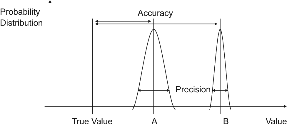
Accuracy and precision. A is more accurate (closer to the true value) but less precise (wider variance). B is less accurate but more precise.

There is also some inherent uncertainty in tests that utilize cutoff points; unless test results are strictly binary, the sensitivity and specificity will vary depending on the cutoff point for the test. Therefore, when thinking about these numbers and conveying the results to patients, it is worthwhile to remember that these probabilities remain estimates.

Multitiered Diagnostic Test Results

Diagnostic tests may have more than 2 levels of results. In the discussion above, FNA was discussed in a simplified form, as though it has only positive and negative results, for the purpose of focusing on binary diagnostic tests. In actuality, thyroid FNA may have 6 potential tiers of results:^10,11 malignant (positive), suspicious (indeterminate), neoplasm (indeterminate), follicular lesion of undetermined significance (includes atypia, indeterminate), benign (negative), and nondiagnostic. Thus, a more robust understanding of FNA results means that sensitivity and specificity go beyond calculating 2 simple fractions, and posttest probabilities cannot simply be calculated with the same formulas discussed in this installment. Thus, evaluating diagnostic tests with multiple tiers will be the topic of the next installment in this series.

Practicalities

One must understand the true nature of these probabilities and their calculations in order to have an accurate understanding of the implications of diagnostic test results. This accurate understanding is necessary to convey correct information to patients. Most clinicians, however, are not innate statisticians who are facile with calculating conditional probabilities. It may be too much to expect clinicians to perform Bayesian or LR calculations every day. Fortunately, there are shortcuts to ascertain the correct probabilities. One such option is in Fagan’s nomogram ( Figure 7 ), which provides a graphical method to determine the correct posttest probability. A second option is to utilize electronic calculators. Such calculators are available online and for handheld devices. (A relatively comprehensive calculator can be found at http://araw.mede.uic.edu/cgi-ebm/testcalc.pl. A calculator with an interactive nomogram can be found at http://www.cebm.net/index.aspx?o=1161. Additional sites with relevant online tools include http://ktclearinghouse.ca/cebm/toolbox/statscalc and http://department.obg.cuhk.edu.hk/researchsupport/Post_test_probability.asp. There are also applications that can be downloaded for the iPhone or iPod: http://appshopper.com/medical/bayes-post-test-probability-calculator.) One can also use these methods to precalculate the probabilities for diagnostic tests that are most frequently used in one’s practice and become familiar with these numbers for regular use. Such precalculations can be performed for a low, intermediate, and high pretest probability (ie, low, intermediate, and high clinical suspicion prior to diagnostic testing, similar to the three clinical scenarios described above) for one’s most commonly used diagnostic tests. While these methods still do require some additional effort, it is a worthwhile investment because they are the means to convey accurate information for ourselves and our patients.

OPEN IN VIEWER

Figure 7.

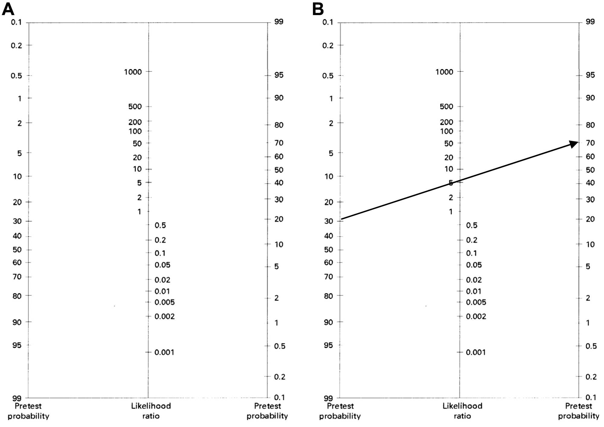
Fagan’s nomogram. (A) The nomogram shows the pretest probability on the left, the likelihood ratio (LR) in the middle, and the posttest probability on the right. (B) A line drawn from the pretest probability on the left, through the LR in the middle, will continue to the right to intersect the nomogram at the level of the anticipated posttest probability. The line demonstrates that a pretest probability of 30% with a LR of 5.7 corresponds to a posttest probability of 71%.

Summary and Conclusion

We frequently use diagnostic tests to guide our impressions of whether true disease is present. Correct interpretation of the results of these tests requires an understanding of predictive values. We must understand predictive values to convey accurate implications of test results to patients. Conveying accurate information to patients is our responsibility and is integral to evidence-based practice.

Author Contributors

Jennifer J. Shin, initial outline, writing on all drafts, data analysis, corresponding author, final approval; Sandra Stinnett, statistical analysis and exposition, writing on drafts, final approval; John Page, epidemiologic analysis and exposition, writing on drafts, final approval; Gregory W. Randolph, intermediate and final draft reviews, revisions for intellectual content, final approval.

Disclosures

Competing interests: Jennifer J. Shin is an editor of Evidence-Based Otolaryngology. John Page is an employee and owns stock in Amgen. Gregory W. Randolph is an editor of Evidence-Based Otolaryngology (Shin J, Hartnick CJ, Randolph G, eds. New York: Springer Science + Business Media, LLC; 2008).

Sponsorships: None.

Funding source: None.