To P or Not to P : Backing Bayesian Statistics

Almost every otolaryngologist spent their formative years becoming familiar with arithmetic, algebra, calculus, and trigonometry—the so-called mathematics of certainty. Then came the numeracy of uncertainty. ¹ We discovered that collecting measurements or counting patients required much more than averages and percentages. Why? Within any system, especially biological systems, there is variability. It is imperative to differentiate what is attributable to chance variation and what is truth before we dare generalize what we see in a sample of subjects to the population at large.

We learned about null hypothesis significance testing (NHST). Strangely, we had to propose our hypothesis (eg, “antibiotics reduce posttonsillectomy hemorrhage”), collect data (eg, retrospective chart review), and then reject some other “null” hypothesis (eg, “antibiotics do not change the rate of posttonsillectomy hemorrhage”) or demonstrate that it was very unlikely. These mental gymnastics made our heads spin. We tried to calculate the probability that the data we had collected could be as extreme as we had encountered (or even more extreme) if the null hypothesis was indeed true. Recall that the null hypothesis was our pet hypothesis’ nihilistic archrival just waiting to rain on our parade. Our hope was that the probability of our data happening by pure chance, if the null hypothesis were true, was too unlikely and therefore the null hypothesis could be rejected.

For decades, research progressed using NHST methods and the P values they generated. Mathematicians and statisticians assure us that these are sound techniques. We feel comforted by the simplicity of a binary decision: accept the null hypothesis if the P value ≥.05 or reject the null hypothesis if the P value is <.05. The .05 number is not a natural constant but a reasonable, although arbitrary, cutoff. Nobody would naïvely believe that a P value of .051 is fundamentally different from a P value of .049, yet our arbitrary dichotomous classification declares that in the first circumstance, we accept the null hypothesis, and in the latter, we reject it. Many a doctor has experienced heightened glee and confidence the lower the P value is. Some statistical packages annotate t tests results with 1, 2, or 3 asterisks (*, **, ***) ² depending on how close the P value approximates .000. A few authors name the levels “statistically significant,” “highly statistically significant,” and “very highly statistically significant” as the P value decreases.^3,4 Alas, there is a major problem. The meaning of P values is misconceived by most. No less than the American Statistical Association issued a statement cautioning against the misuse of P values. ⁵ A smaller P value does not mean a larger effect of whatever is investigated, nor does a P value measure the importance of a result. A researcher, striving to tell a story, can be tempted to “P hack,” where he or she spuriously contrasts factors with a P value <.05 against those factors whose P value is >.05. We now live in the era of big data in which we frequently have thousands of cases with hundreds of variables and, in the case of genetics, millions of variables. Such data lend themselves to a panoply of depressed P values that are probably meaningless.

NHST and P values are the outputs of a branch of statistics called “frequentist statistics.” Another distinct frequentist output that is more useful is the 95% confidence interval. The interval shows a range of null hypotheses that would not have been rejected by a 5% level test. In other words, it gives us a feeling of the potential magnitude of an effect, otherwise known as the parameter estimate. A parameter estimate might refer to a continuous parameter such as a concentration expressed in mg/mL or a frequency parameter such as the incidence of a particular complication in a cohort of patients. We, and many statistically educated individuals, succumb to temptation by interpreting the 95% confidence interval as if there was a 95% chance that the true estimate falls in that range. This is not what a 95% confidence interval actually means, but fortuitously, in many situations, that notion does hold true. The 95% confidence interval from our particular sample is merely just one range whereby 95% of such samplings would generate an interval that would include the true parameter. The implication is that 5% of such intervals would not include the true value of the parameter. Once again, our heads spin. Wouldn’t it be nice if instead of working backward, calculating the probability of getting the data we got if the null hypothesis were true, we could instead work forward by calculating the probability of our hypothesis given the data?

Bayesian statistics, in common with frequentist statistics, provide us with an estimate of a parameter. For instance, we can estimate the change in hearing loss or the percentage of patients who develop a cerebrospinal fluid (CSF) leak following a procedure. Only Bayesian methods will give a probability distribution for a parameter. In other words, we can ascribe a probability to our best estimate and to all the possible values of the parameter. Furthermore, we can start with a blank slate where everything is possible and all possibilities are equally likely, or we can start with our beliefs from data collected during previous studies.

Our starting beliefs are called prior probabilities. We then collect and enter our data. A common workflow would proceed with our computers executing a sampling algorithm that randomly runs through the data thousands of times to determine how likely or unlikely a particular event or a particular parameter value is. The results of all simulations are assembled to provide a posterior probability in the form of a probability distribution. We can directly read the most probable estimate of the parameters. We can directly read where 95% of the simulations end up and thereby declare a 95% credible interval that genuinely is an interval in which there is a 95% probability of the true population estimate falling (in contrast to the 95% confidence interval).

For instance, let us assume that 2 interventions to improve hearing are being compared. They may be clinically equivalent if the absolute difference is ≤6 decibels. We can declare the whole region from −6 dB (“orange” intervention negligibly better than “blue” intervention) to +6 dB (“blue” intervention negligibly better than “orange” intervention) to be the region of practical equivalence (ROPE). We can then directly read the number of simulations that fall inside the ROPE and, more importantly, the number that fall outside of the ROPE. In so doing, we can declare the probability that one intervention is actually clinically superior to another (see Figure 1 and Figure 2 ). The posterior probability then serves as the prior probability when more data become available and then we can update the posterior probability.

OPEN IN VIEWER

Figure 1.

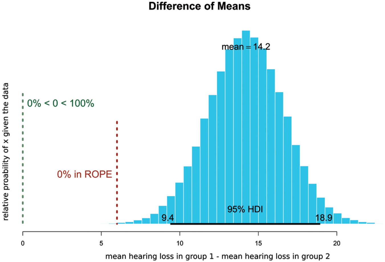
Comparison of hearing loss in 2 simulated groups that are statistically significantly different and are not clinically equivalent. The graph is the probability, on the y-axis, of each possible value of mean difference, given the data.^10-12 HDI, high-density interval; ROPE, region of practical equivalence.

OPEN IN VIEWER

Figure 2.

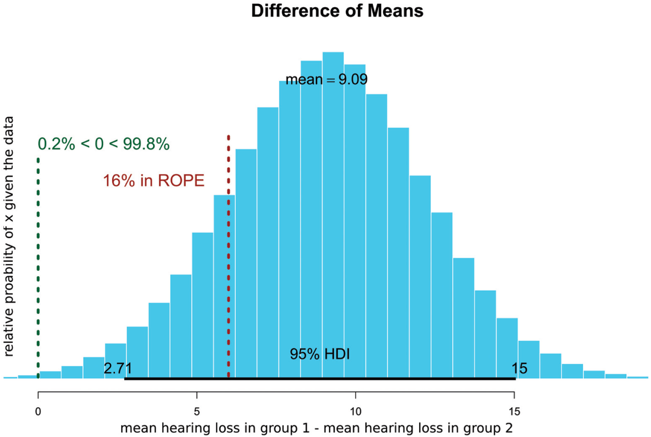
Comparison of hearing loss in 2 simulated groups that are statistically significantly different but may be clinically equivalent. Ten percent of the probability distribution is in now in the ROPE. HDI, high-density interval; ROPE, region of practical equivalence.

Attempts are being made to deal with limitations and misinterpretations of frequentist statistics. Some are radical such as the recent ban on P values and NHST by the Journal of Basic and Applied Social Psychology. ⁶ As published research is full of significance tests, clinicians and researchers will continue to be confronted by their use, and discarding them altogether may not be the answer, particularly without education increasing on the usage of Bayesian methods. For most otolaryngologists, putting Bayesian methods into practice is a challenge. The adoption of Bayesian statistics is relatively new, and even recently graduated trainees are unfamiliar with the principle, whereas frequentist NHST remains familiar. Taking courses or working with a statistician will decrease gaps in knowledge. A good starting place for the interested reader are gentle introductions to Bayesian analysis by van de Schoot et al ⁷ and Spiegelhalter et al. ⁸ Regardless of familiarity, specifying a prior probability has many pitfalls. We have to decide what our prior beliefs are. For example, when considering the incidence of CSF leaks following translabyrinthine skull base surgery, we may start with a prior probability in which every incidence from 0% to 100% is equally likely ⁹ : a uniform distribution. Alternatively, we may specify that some incidences are more likely than others (eg, incidences between 2% and 25% are much more likely than those around 60% and above). Skill, art, and subjectivity are all brought to bear on the process by which our subjective belief is translated into a mathematical model. Furthermore, Bayesian statistics, especially when using complex models and involving many variables, is computationally intensive.

In summary, frequentist NHST is not wrong, but its results are susceptible to confident misinterpretation. Bayesian statistics provide direct answers to how confidently we should believe what we believe. It is time to embrace and encourage the use of these methods in our otolaryngology research.