
Abstract
This paper studies the forecast accuracy and explainability of a battery of dayahead (Henry Hub and Title Transfer Facility (TTF)) natural gas price and volatility models. The results demonstrate the dominance of non-linear, non-parametric models with deep structure relative to various competing model specifications. By employing the explainable artificial intelligence (XAI) approach, we document that the price of natural gas is formed strategically based on crude oil and electricity prices. While the conditional volatility of natural gas returns is driven by long-memory dynamics and crude oil volatility, the informativeness of the electricity predictor has improved over the most recent volatile time period. Although we reveal that predictive non-linear relationships are inherently complex and time-varying, our findings in general support the notion that natural gas, crude oil and electricity are interconnected. Focusing on the periods when markets experienced sharp structural breaks and extreme volatility (e.g., the COVID-19 pandemic and the Russia-Ukraine conflict), we show that deep learning models provide better adaptability and lead to significantly more accurate forecast performance.
Keywords
1. Introduction
An accurate forecasting model for natural gas price is essential not only for gas trading, but also for gas production, storage, and distribution. Economic planning, investments in the energy sector, and environmental protection represent additional activities that may rely on accurate gas price forecasting. Considering the increased construction rate of gas-fired power plants over the past 10 years, such a model could assist government policy-makers in their planning efforts for electric power production and market design.
Within the boundaries of Central and Western European natural gas markets, it is common to price long-term natural gas contracts by using an oil-indexed formula (Fiorenzani et al., 2012). 1 This formula ties the natural gas price to the price of alternative fuels, namely crude oil and its derivatives (heating oil, diesel, etc.). Such a traditional approach to modeling natural gas prices is rooted in the phenomenon that natural gas was often a by-product of crude oil exploration and due to the fact that natural gas and oil are related in terms of consumption. If we assume that the oil-indexed formula contains n factors, the price of natural gas at time t (Pt) can be generally expressed as follows (Franza, 2014; Tusiani and Shearer, 2007):

where P0 is the contracted (base) price of natural gas at time 0, ωi’s (i = 1,…,n) are weighting factors that define the relative contribution of each of the n factors (alternative fuels) to the pricing formula, βi’s (i = 1,…,n) are linear regression coefficients that represent slope parameters for the factors Fi (i = 1,…,n), Fit is the price of factor i at time t, while Fi0 is the (base) price of factor i at time 0.
A panel of possible n predictors (i.e., factors) in the model may include crude oil price, fuel oil with a maximum sulfur content of 1% (or 3%), coal price, and diesel gas price. The factors Fit are estimated as moving averages on the time interval from 0 to t, where t could range from three to nine months (Gerner, 2010). For example, the factor prices are averaged over a period of nine months in Russia and the Republic of Serbia.
This paper analyzes the viability of a more general, non-linear model specification for forecasting natural gas price in the U.S. market. Such a model can be written as

where ΔPt is the change in the logarithm of natural gas price over a certain time period (e.g., daily), i.e., ΔPt = ln(Pt) - ln(Pt–1), while ΔFit’s are the logarithmic changes of the predictors. 2 In this context, our paper relies on a non-linear model architecture that allows for rather complex relationships between predictors and the dependent variable, non-normality of gas price return distributions and, also, facilitates adaptive learning. 3
It is important to stress that the motivation for introducing electricity as an additional predictor stems from its increased interconnections to natural gas pricing and consumption over recent years. For instance, the share of electricity generation from natural gas has increased from 14% to 23% over the past 35 years, while the corresponding shares from oil and coal have declined from 11% to 3% and 38% to 36%, respectively. 4 The informativeness of crude oil price, as a main factor in the oil-indexed formula, has been researched in the past (e.g., Ji et al. 2018; Asche et al. 2017; Nick and Thoenes 2014; Brown and Yücel 2008), but the literature has been relatively silent on the role of electricity in gas price formation. In addition, to the authors’ best knowledge, none of the previous scholarly works have attempted to explain the complex non-linear relationships inherent in gas price and volatility forecasting by using the explainable artificial intelligence (XAI) method.
In general, our paper fits within the active research area of natural gas price forecasting that has received additional attention due to the recent downturns in energy markets. In a seminal paper, Buchanan et al. (2001) utilized natural gas futures market positions of large hedgers and speculators to find that weekly spot gas prices are inefficient in the semi-strong form. Furthermore, Mishra and Smyth (2016) could not forecast daily Henry Hub natural gas spot prices by using futures prices better than a random walk. Among other predictors, the information from forward contract prices was also explored in Nguyen and Nabney (2010). They combined wavelet transform with non-linear models (multi-layer perceptron, radial basis function, and GARCH) and concluded that wavelets in general improve point forecasting for the U.K. daily gas prices. Salehnia et al. (2013) extended the set predictors of spot gas prices for several non-linear models including artificial neural networks (ANNs) that stood out as the most accurate (day-ahead) forecasting method. Similarly, Čeperić et al. (2017) enhanced the support vector machine and ANN models with a feature selection algorithm to improve one-day-ahead (and one-week-ahead) Henry Hub spot price forecast accuracy. They identified a few informative predictors (e.g., heating oil prices, total U.S. market natural gas production, the U.S, natural gas rotary rig count and coal prices), but they did not rank them according to their non-linear importance in the models. The results of Čeperić et al. (2017) essentially confirmed those of Busse et al. (2012) for the German market: ANN natural gas forecasting models were only marginally dominant when compared to traditional time-series methods (e.g., AR and ARIMA) and the random walk model. Recent scholarly contributions such as Su et al. (2019) and Mouchtaris et al. (2021) also stressed the usefulness of ANN (machine learning) models in predicting natural gas prices. 5
This paper complements existing literature by introducing original predictors (electricity prices, air temperature, prices of fuel oils of various sulfur content) and by employing a multitude of linear and non-linear models (deep ANN, random forest, extreme gradient boosting, lasso, ridge and elastic net model). Moreover, we assess the relative importance of the non-parametric models’ inputs via the XAI methods. Put differently, we evaluate and rank the non-linear importance of predictors in forecasting natural gas prices and volatility. Much of the literature has dealt with the input selection problem by using input selection algorithms (e.g., Čeperić et al. 2017) or by testing ˇ alternative model variants (e.g., Nguyen and Nabney, 2010), but a predictor’s relative impact on the model’s output has never been gauged. This exercise allows us to interpret results theoretically, in terms of the potential shift from traditional oil-indexed formula to a new pricing paradigm.
We find that our non-linear model specifications are superior to the linear model (and the benchmarks: random walk model and AR(1)), while the best performing model is an ANN model with deep structure. In terms of the inputs’ significance, we report that the most important predictors for gas returns (Henry Hub and TTF) are crude oil price, temperature and electricity price. The corresponding set of volatility predictors does not perform as well on the 2015–2020 data, except for the crude oil volatility that nicely complements the long-memory characteristics of natural gas conditional volatility. It is worthwhile to note that the price (volatility) of European Emission Allowances (EUA) has emerged as the second most (the most) informative predictor for the TTF Hub natural gas price (volatility). Taken together, our results suggest that traditional oil-indexed pricing formula has evolved to incorporate electricity price as an equally important input. 6 Even though we do not empirically test causality direction between gas and electricity prices, we show that electricity prices act as one of the most informative predictors for natural gas prices, and to a lesser extent for the conditional volatility.
Extending our empirical framework, we further explore the predictive performance of the models during the periods of the COVID-19 pandemic and the Russia-Ukraine crisis. Our findings reveal that, during such periods when sharp structural changes and extreme uncertainty occur in the market, deep learning models provide better adaptability and lead to significantly better forecast performance. This highlights the potential advantages of using AI-based methods for accommodating the dynamics of energy markets.
The remainder of the paper is laid out as follows. In Sections 2 and 3, we describe the methodology and the data, respectively. Sections 4 and 5 present the results of our empirical analysis, while Section 6 outlines the predictive performance of models during the COVID-19 pandemic and the Russia-Ukraine crisis. Section 7 concludes the paper.
2. Methodology
2.1 Feedforward Deep Artificial Neural Network (FF-D-ANN)
To explain the concept of an FF-D-ANN model, we will assume that natural gas returns at time t + 1 (ΔPt+1) are forecasted by n predictors or factors (ΔF1t,i = 1,…,n), and that this mapping is a non-linear function (ϕ) whose parameters will be estimated (i.e., ΔPt+1 = ϕ(ΔF1t, ΔF2t, …, ΔFnt)). The parameters are called connection weights (αij and βj) and node biases (αj0 and β0). Figure 1 shows the structure of an FF-D-ANN model that is used to approximate the non-linear mapping. It consists of three building blocks that are the input layer (where predictors are fed into the model), hidden layers (where the functional approximation or learning takes place) and the output layer (where the gas returns forecast is generated).
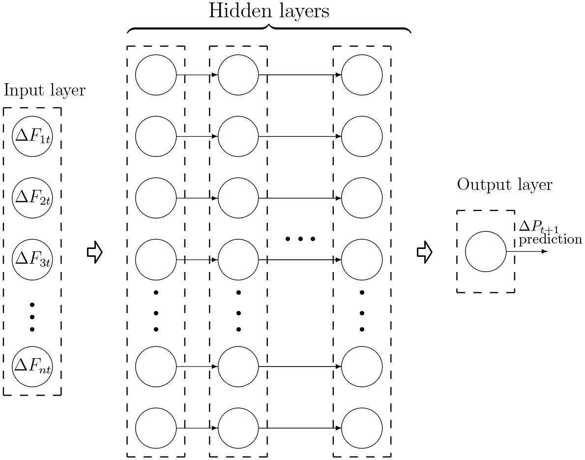
Feedforward deep learning artificial neural network (FF-D-ANN) model
If we initially assume the model architecture involves only one hidden layer with q computational elements (nodes or neurons), the FF-D-ANN model is estimated as:
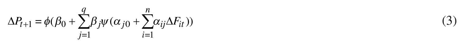
In this example, q is the number of hidden nodes, where the single hidden and the output layers are characterized by two flexible classes of non-linearities: ψ and ϕ, respectively. αij and βj denote appropriate connection weights between the adjacent layers. Subscripts 0 for α and β stand for the biases. When it contains multiple hidden layers, this model is also called a multilayer perceptron (MLP). In such a case, Equation 3 becomes more complex with more non-linearities nested in each other. Nevertheless, the logic of transforming inputs into each node by taking their weighted average, adding biases, and non-linearly transforming the sum (that is passed forward to the subsequent layer’s nodes) still applies. It is worthwhile to stress that a multilayered model structure with at least two hidden layers is what facilitates ‘deep learning’ in practical applications. In our model design, we rely on complex D-ANN models that can extract predictive information from a variety of inputs (lagged factors), while utilizing a deep structure with multiple hidden layers.
The training algorithm is Adam, a deep learning first-order gradient-based optimizer based on adaptive estimates of lower-order moments. It is computationally efficient and suitable for large datasets with a lot of parameters to estimate. The default parameters follow those provided in Kingma and Ba (2015). The activation function types used in the hidden layers are sigmoid, with the linear function in the output layer. To control for overfitting, we use a 10% dropout. Validation data is used to select the optimal model architecture. The model will set apart 10% of training data, will not train on it, and will evaluate loss (i.e., mean-squared error) and any model metrics on this data at the end of each epoch. If, during the last 5 epochs monitored quantity (validation loss) has no improvement, training will be stopped.
2.2 Random Forest (RF) Model
A random forest (RF) is an ensemble machine learning technique introduced by Breiman (2001). It consists of a collection of regression trees whose averaged outputs determine the final prediction of the ensemble. RF learning is based on an extension of bootstrap aggregation (bagging) using random features subspace selection. Through a bagging procedure, each tree in the ensemble has randomly selected portions of training samples (with replacement) from the original dataset.
However, in order to avoid possible correlations between constituent random trees and enhance the estimation performance of the RF model, the idea of a random features subspace is introduced. As a result, each tree is grown on the basis of a randomly chosen input subset. For each node, the splitting algorithm searches over a subset of selected features to determine the best split point. The algorithm continues splitting new nodes until a stop criterion is reached, e.g., the number of instances of the node is less than a preset number. RF growth during the learning process is determined by two parameters: the size of the features subset used in each regression tree and the number of trees that form the forest. In our implementation, we select the features subset size as the first integer lower than log2n + 1, where n is the number of inputs (ΔFit,i = 1,…,n), while 80 trees were adopted to build the RF structure. 7
In the process of constructing each decision tree by splitting its nodes into descendant ones, the RF learning algorithm uses the classification and regression trees (CART) learning algorithm (Breiman et al., 1984) which adopts the Gini index as the impurity-based measure (classification), or a “goodness of fit” measure (regression). In the regression context, a typical splitting criterion is the sum of squared residuals at the node where the optimal cut-off point is determined on the basis of evaluation of splits between every distinct pair of consecutive values. For a given input vector x, the final RF regression prediction
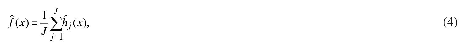
where
2.3 LASSO, Elastic Net and Ridge Regression
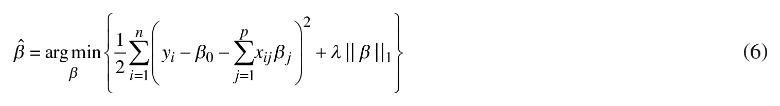
The least absolute shrinkage and selection operator (LASSO) model is a variant of the least squares regression that constrains the sum of the absolute values of regression coefficients as follows (Hastie et al., 2015):
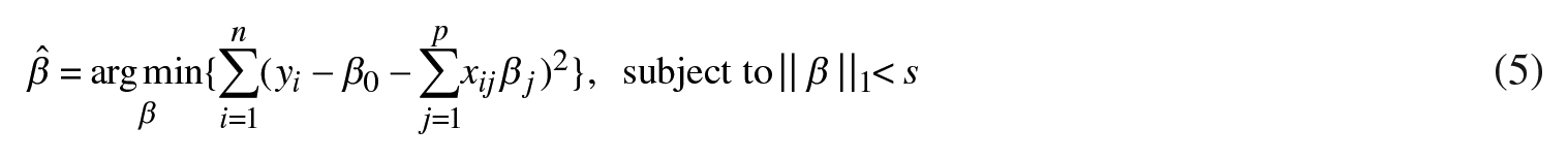
where yi is the ith observation of the dependent variable, β0 is an intercept, xij is the ith observation of the jth predictor and βj’s are the corresponding coefficients,
When s becomes large, the constraint ||β||1< s has no effect and the model becomes a standard linear regression. However, for sufficiently small (but positive) values of s, the estimated parameters (βj) are reduced when compared to the least squares method’s counterparts, while certain parameters βj are often equal to zero. The cross-validation method is typically used to find the optimal value of s (and, also, for the parameter λ below) and, thus, this paper will follow the same approach.
Also, the LASSO optimization problem can be written in a Lagrangian form:
Henceforth, the LASSO regression will be estimated by using the coordinate descent algorithm that includes two steps (Friedman et al., 2007): 1) λ will be estimated via ten-fold cross-validation and 2) based on the estimated λ, βj’s will be estimated.
To forecast natural gas returns, we also include the elastic net method in our set of competing predictive models. This model is considered an improvement over the LASSO regression as it introduces additional constraints on the regression coefficients in the following manner (Zou and Hastie, 2005):
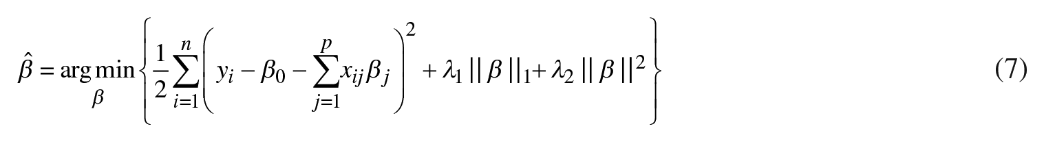
Elastic net was developed to tackle the issue of potential significant correlations among regression predictors and improve the forecast ability of the LASSO approach.
In our efforts to improve the least squares method, the final comparative model that will be tested is the ridge regression (Hoerl and Kennard, 1970). This model is the least complex in regards to the constraints imposed on the regression coefficients whereas only the L2 norm is used:
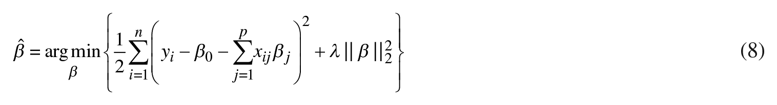
At the heart of the ridge method is the technique that alleviates the problem of high degree of multicollinearity among the predictors. It is aimed at improving the forecast accuracy of linear models and is often used as an alternative to a simple linear regression.
3. Data Description
The data were sampled daily and collected from the Bloomberg platform. Our sample covers the periods 2015–2020 in the first part of the analysis that concerns only Henry Hub, but that both TTF and Henry Hub (returns and volatility) are forecasted on the expanded more recent data spanning the years 2020–2022. The dependent variable is the spot natural gas (Henry Hub) returns calculated as ΔPt = ln(Pt) – ln(Pt–1). The predictors (in first differences), selected on the basis of theoretical and empirical considerations from the literature and data availability, are as follows: heating oil prices (New York Harbour)(Δhoil), crude oil prices (WTI Crude Oil)(Δcoil), fuel oil with the up to 1% sulfur content prices (New York Harbour)(Δfoil1p), fuel oil with the up to 3.5% sulfur content prices (New York Harbour)(Δfoil35p), diesel gas with ultra low sulfur prices (Gulf Coast)(Δdiesel), electricity prices (PJM West)(Δelec), and temperatures in Fahrenheit (New York State)(Δtemp).
We begin our analysis by displaying the summary statistics for each time series. Table 1 shows that the average return for all variables is small, which suggests that the prices were relatively stable during the 2015–2020 period. 8 However, except for the gas returns, the differences between arithmetic means and medians are in some cases noticeable. Specifically, the median is greater than the mean for heating oil, diesel, crude oil and temperature. This may indicate a negatively skewed distribution of returns, but the skewness coefficient is within the (–0.5, +0.5) interval in all cases; thus, the distributions appear to be mostly symmetric. Next, we can observe that the standard deviations are small which confirms the data period had not much volatility. Finally, the kurtosis figures for the predictors point to leptokurtic distributions that significantly depart from normality. 9
Summary statistics
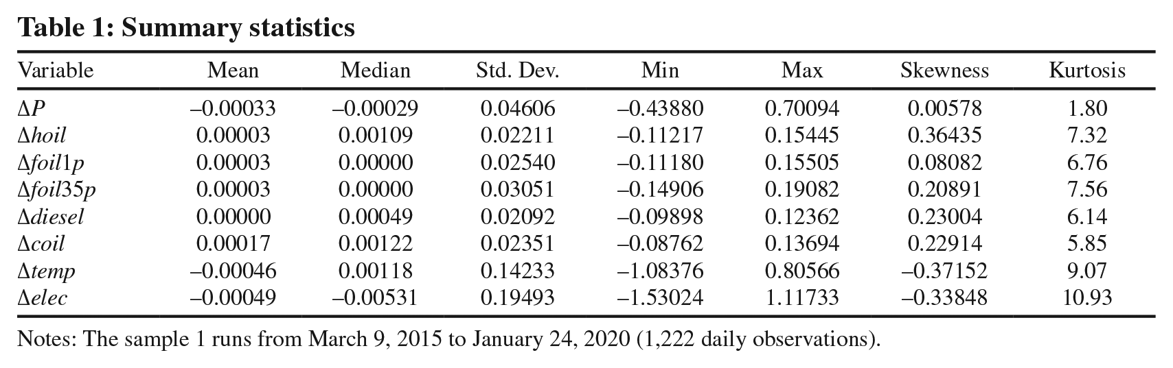
Notes: The sample 1 runs from March 9, 2015 to January 24, 2020 (1,222 daily observations).
In the last part of our data description, we will run a simple linear regression model. This will allow us to understand the nature of the linear relationship between each predictor and gas price movements. Table 2 presents the estimates of the following contemporaneous regression 10 :

Linear regression estimates
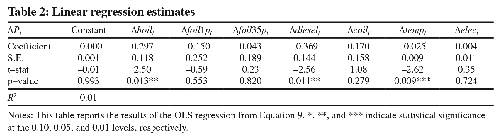
Notes: This table reports the results of the OLS regression from Equation 9. *, **, and *** indicate statistical significance at the 0.10, 0.05, and 0.01 levels, respectively.
Table 2 demonstrates the inability of the linear model to explain gas price fluctuations (R2 = 0.01). The statistically significant estimates were β1 (Δhoilt; at the 5% significance), β4 (Δdieselt; at the 5% significance) and β6 (Δtempt; at the 1% significance). Gas prices are inversely related to air temperature (β6 < 0). These results emphasize that a linear model specification is inappropriate and, in our further empirical work, we turn our attention to non-linear models.
4. Empirical results: Forecasting returns
The competing models with seven lagged predictors (as in Equation 2) will be estimated based on the first 80% of our data set (i.e., the training data set) or 977 days. The remaining data are used for model validation (10%) and testing (10%). This leaves 122 observations out-of-sample for which we compare the one-day-ahead forecast performance of the following models: FF-D-ANN, RF, random walk (RW) model, linear model (LINEAR), AR(1), ridge regression (RIDGE), lasso regression (LASSO), and elastic net (ELASTIC) regression.
The RW model is specified as follows:

where ΔPt denotes the natural gas log-returns. We generally use a “driftless” form of the RW model (α = 0).
The optimal model architecture (obtained from the validation data) for the FF-D-ANN model is “7-22-14-1”, i.e., two hidden layers with 22 and 14 neurons, respectively. The RF model was specified as explained in subsection 2.2. We estimate the LASSO, RIDGE and ELASTIC models by using the coordinate descent algorithm that involves two stages (Friedman et al., 2007). In the first stage, we estimate the tuning parameters (α and/or λ) with ten-fold cross-validation on the in-sample data. In the second stage, from the estimates of the tuning parameters, we estimate the vector of regression coefficients, and then generate out-of-sample forecasts.
Table 3 shows the statistical accuracy reflected in the mean squared prediction error (MSPE) and the mean absolute prediction error (MAPE) of the models that were tested on out-of-sample data. We find evidence of non-linear one-day-ahead predictability of natural gas returns. The FF-D-ANN model produces the most accurate forecasts; it is able to improve upon the RW and LINEAR models by about 4–6% in terms of the MSPE and by about 3–4% in terms of the MAPE. A surprising finding is that the RF underperformed relative to the FF-D-ANN model. It is also striking that the LINEAR and AR(1) models performed the poorest. The alternatives to the LINEAR model (LASSO, RIDGE and ELASTIC) show marginal improvements and are in general inferior to the RW model. Clearly, it is imperative to rely on a non-linear model specification when forecasting natural gas price fluctuations.
Comparison of predictive models for returns
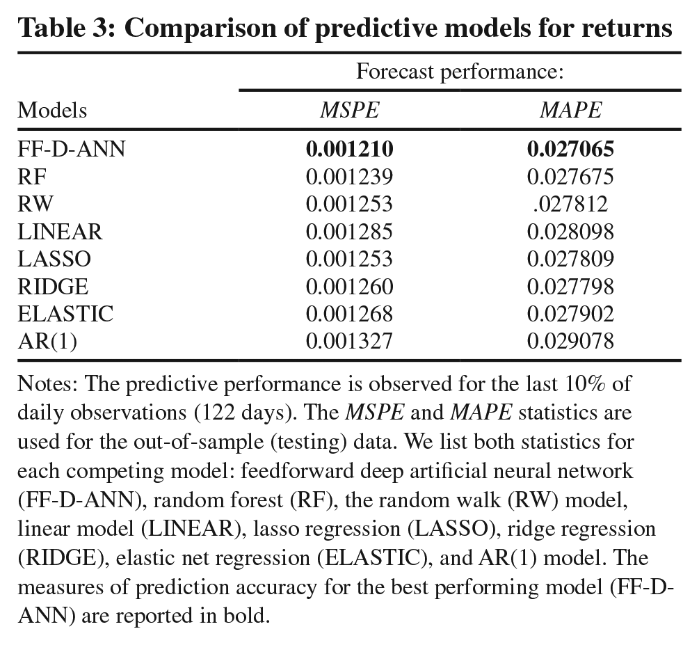
Notes: The predictive performance is observed for the last 10% of daily observations (122 days). The MSPE and MAPE statistics are used for the out-of-sample (testing) data. We list both statistics for each competing model: feedforward deep artificial neural network (FF-D-ANN), random forest (RF), the random walk (RW) model, linear model (LINEAR), lasso regression (LASSO), ridge regression (RIDGE), elastic net regression (ELASTIC), and AR(1) model. The measures of prediction accuracy for the best performing model (FF-DANN) are reported in bold.
Considering that non-parametric, non-linear models have often been blamed for their lack of economic interpretability, next, we tackle this problem by using the XAI approach. More precisely, the increased model complexity obscures the understanding of which predictors influence the model. However, managers in the gas industry need to know what to base their decisions on. To quantify the non-linear importance of the predictors (or features), first, we will utilize the method of pseudo-weights proposed by Qi and Maddala (1996). This will enable us to identify the non-linear economic importance of the inputs of the FF-D-ANN model. Basically, the weighted average of the input weights is used to find the marginal contribution of each input variable to the output. The formula for a pseudo-weight for the ith input (PWi, i = 1,…,k) of a FF-D-ANN with n hidden layers can, in general, be written as
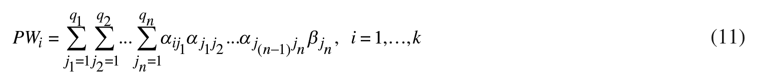
where q1,q2,…,qn is the number of nodes in each of the n hidden layers;
Then, we will compare the results obtained from the pseudo-weights to the Gini indices estimated from the RF model. The Gini index describes a decrease in the RF node impurity weighted by the probability of reaching that node:
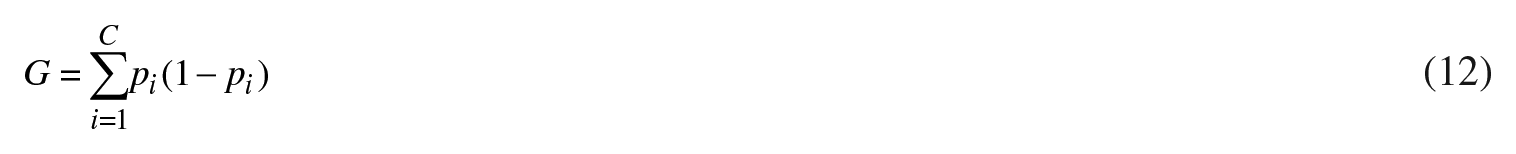
where pi is the node probability calculated as the number of observations that reach the node divided by the total number of observations and C is the number of classes in the target variable. Feature importance in the form of Gini index is commonly used to identify the contribution of individual predictors toward explaining the output (natural gas daily returns).
Table 4 lists seven inputs along with their corresponding estimated (in-sample) pseudo-weights (PWi, i = 1,…,7) and Gini indices (Gi, i = 1,…,7). Over the whole data range of almost five years of pre-COVID-19 pandemic observations, it transpires that natural gas prices have been mostly driven by the price of electricity, followed by the crude oil price and temperature. The other predictors have a substantially lower impact on gas prices. It appears that natural gas prices are strategically formed based on crude oil and electricity prices. The fact that the evidence from the pseudo-weights is similar to that from the Gini indices adds to the strength of the results and the validity of our approach.
Relative contribution of predictors
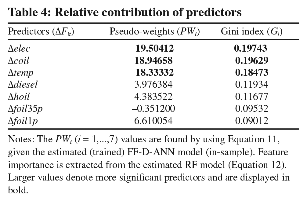
Notes: The PWi (i = 1,…,7) values are found by using Equation 11, given the estimated (trained) FF-D-ANN model (in-sample). Feature importance is extracted from the estimated RF model (Equation 12). Larger values denote more significant predictors and are displayed in bold.
Finally, we expand the XAI analysis by introducing the Shapley additive explanations (SHAP) values for our set of inputs (Lundberg and Lee, 2017). The advantage of this method lies in its ability to explain the output of any machine learning model. Essentially, the SHAP values show how much each predictor contributes (positively or negatively) to the output. Another benefit of the SHAP approach is its local interpretability where each observation is assigned its own set of SHAP values. In contrast, pseudo-weights and Gini indices only average the results across the entire data set, but they do not focus on individual observations or subsets of data. First, we will estimate the SHAP values across the whole training data set for the RF model by taking (1) the mean absolute value of each feature (Figure 2: Panel A) and (2) the maximum absolute value of each feature (Figure 2: Panel B).
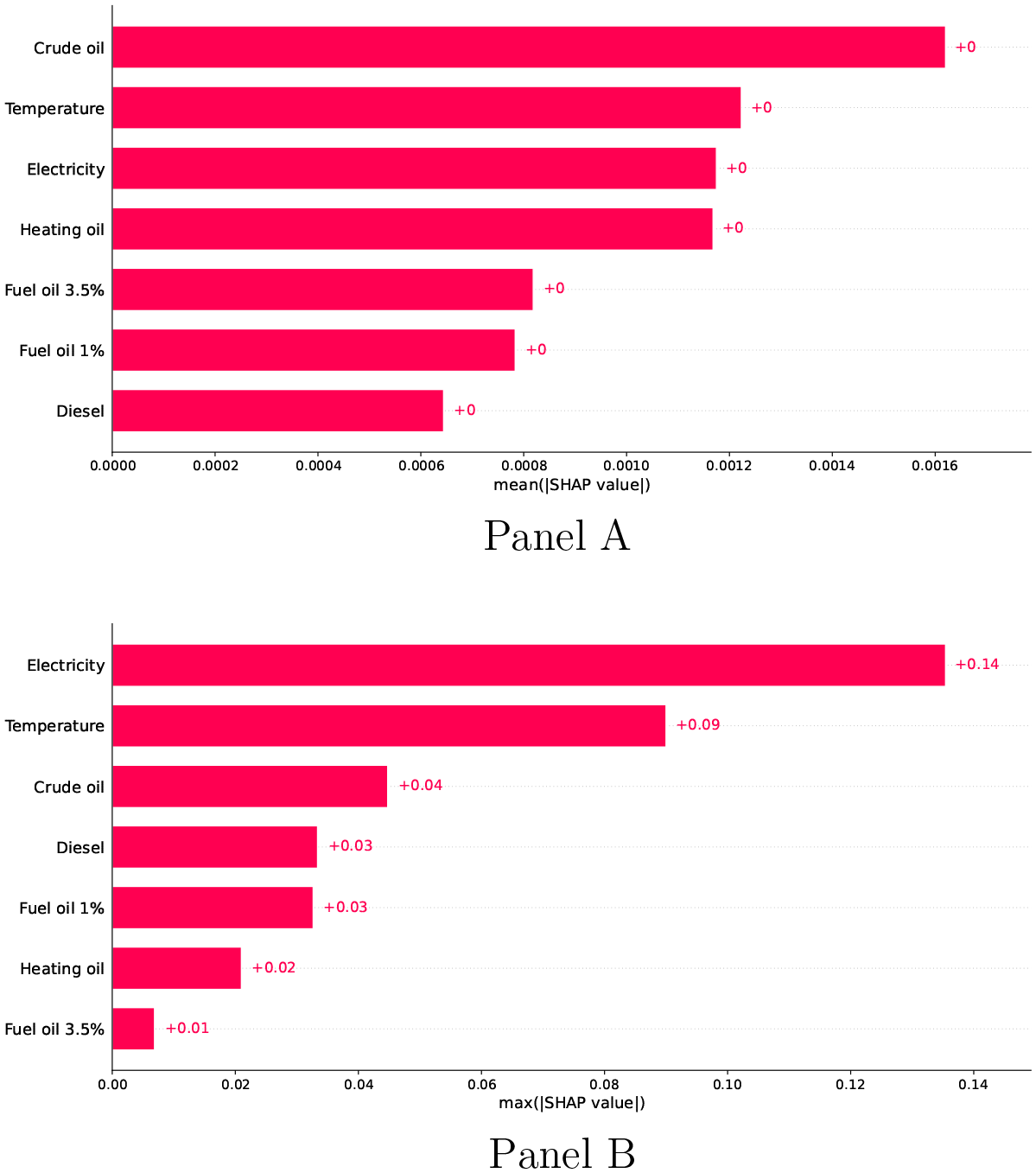
SHAP values - bar plot
Figure 2 (Panel A) demonstrates the key role that crude oil price, electricity price and temperature play in forecasting natural gas prices. When compared to our previous findings, crude oil price emerges as the driving force for gas price changes, while heating oil price becomes as important as electricity price. It is worthwhile to note that such results are based on the mean absolute value of all training instances, i.e., they represent aggregate measures of feature importance. On the contrary, when we used the maximum absolute value of the features, the evidence presented in Figure 2 (Panel B) suggests that electricity price has the most pronounced impact on gas prices. This can be interpreted as a series of extreme effects that electricity prices may occasionally exert on gas prices. Hence, although, on average, crude oil price is the most dominant factor, electricity prices seem to be related to stronger movements in gas prices. In addition, according to the SHAP values plotted in both panels of Figure 2, with respect to the three most significant factors, the results are consistent with those from Table 4.
To obtain deeper insights into the relative importance of predictors, we visualize the magnitude of each feature by using a heatmap plot (Figure 3). The heatmap shows the relationships in two dimensions. The predictor importance is shown in descending order on the vertical axis, while the observation (instance) number of training data is on the horizontal axis. Specifically, the SHAP values are found for each instance-input combination and their relationship to the output is denoted by red (direct relationship) or blue (inverse relationship) rectangles. It can be observed that higher values of gas returns are mostly associated with higher values of electricity returns (i.e., red color). The relationship is remarkably stable across time. In contrast, the relationship between gas prices and temperature is generally negative, i.e., blue colored rectangles are dominant in the second row of the heatmap. It is intriguing to report that such relationships are in accord with the results from the linear model (Table 2).
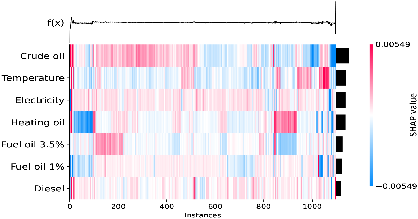
SHAP values - heatmap
The association between natural gas and crude oil is, however, more complicated. In particular, the observed negative association requires more care to interpret. First, by plotting the price of natural gas alongside crude oil price in Figure 4, one can notice they initially moved in tandem, but the decoupling of oil and gas prices took place in late 2017. At the same time, the U.S. shale gas and oil production both experienced declines between the years 2015–2017, while they picked up in the third quarter of 2017 and have been steadily increasing ever since. 11 We speculate that fluctuations in U.S. shale production caused the decoupling of oil and gas prices, as indicated by the heatmap in Figure 3. Essentially, weak (strong) regional natural gas supply from shale production facilitates coupling (decoupling), because oil is a global commodity. 12
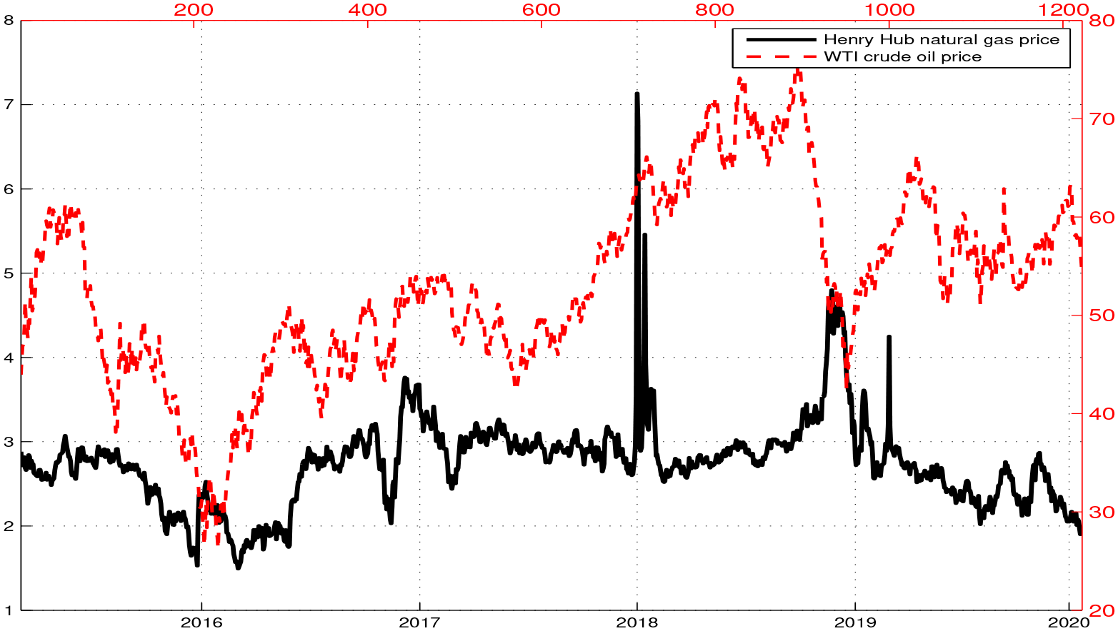
Natural gas and crude oil time series plot
5. Empirical results: Forecasting volatility and dynamic interactions
Having assessed the performance of non-linear models for forecasting natural gas prices, we now extend our framework and look into volatility forecasting. 13 We proceed as follows. First, in the next subsection, we estimate a conditional volatility model which permits incorporating various forms of empirical features embedded in the volatility of gas prices (such as long memory, volatility clustering, fat tails, effects of asymmetric shocks and returns). Upon fitting the model, we obtain the time series of (in-sample) conditional volatility and use it as input for our (out-of-sample) forecasting procedures. Second, next to our volatility prediction analysis, we revisit in subsection 5.2 our discussion pertaining to the relationship between natural gas and crude oil. In particular, we reassess patterns revealed in Figure 4 and estimate dynamic correlations as well as covariances between these two variables. Finally, subsection 5.3 presents our forecasting results for conditional volatility measures, based on a set of advanced non-linear models.
5.1 Conditional Volatility
To estimate conditional volatility of natural gas prices, we estimate a FIEGARCH (1, d, 1) model with three explanatory variables (in the variance equation): temperature, crude oil and electricity. The model allows us to accommodate volatility clustering, long memory, effects of shocks in terms of sign and magnitude, and we estimate the model using the Student’s t distribution to account for fat tails. 14
Table 5 presents model specification and reports estimation results. Several findings stand out. First, consistent with the well-known stylized characteristics of financial assets (e.g., stocks, bonds and exchange rates), volatility of natural gas exhibits significant volatility clustering (i.e., ARCH and GARCH effects). 15 There is strong evidence of long memory (d = 0.657) and the assumption of normal distribution is clearly rejected (υ = 5.298). Interestingly, the estimated coefficients of the explanatory variables x1, x2 and x3 (crude oil, temperature and electricity) are statistically insignificant and hence they fail to influence conditional variance of natural gas. 16 Moreover, we find no evidence for asymmetric (i.e., negative vs. positive) effects of shocks on volatility, thereby there is no sign effect, as the first coefficient of the EGARCH component (γ1 = −0.007) is not statistically significant. The magnitude effect appears to be considerably significant (γ2 = −0.443), however, which suggests that larger shocks hitting natural gas tend to increase conditional volatility over time. 17
Estimation results of FIEGARCH (1, d, 1) model for natural gas returns
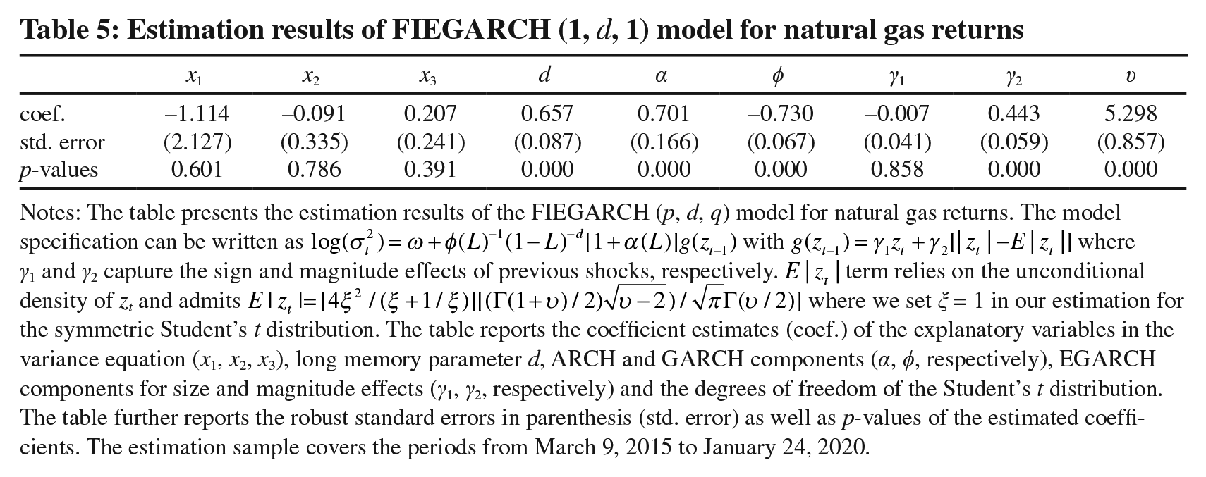
Notes: The table presents the estimation results of the FIEGARCH (p, d, q) model for natural gas returns. The model specification can be written as
5.2 Dynamic Correlations and Covariances
In addition to our assessment of conditional volatility dynamics, we now closely explore the link between natural gas and crude oil in light of the regularities highlighted in Figure 4. For this objective, we estimate a dynamic conditional correlation (DCC) model based on the previously used FIEGARCH specification with the multivariate Student’s distribution. After fitting the model, we compute the dynamic correlations as well as covariances between crude oil and natural gas over the full sample.
As displayed in Figure 5 (left panel), the correlation between natural gas and crude oil is relatively time-varying and asymmetric over the business cycle. 18 It is also noticeable that correlations exhibit swift ups-and-downs and that pattern is potentially attributed to market conditions, as discussed earlier, affecting (both) crude oil and natural gas. While the correlation is mostly positive during the first half of 2018, we observe a negative correlation in late 2018 with a large downward spike occurring in November 2018. It is, nevertheless, worth mentioning that these daily correlations vary between –0.10 and 0.14 and hence appear to be weak in most periods.
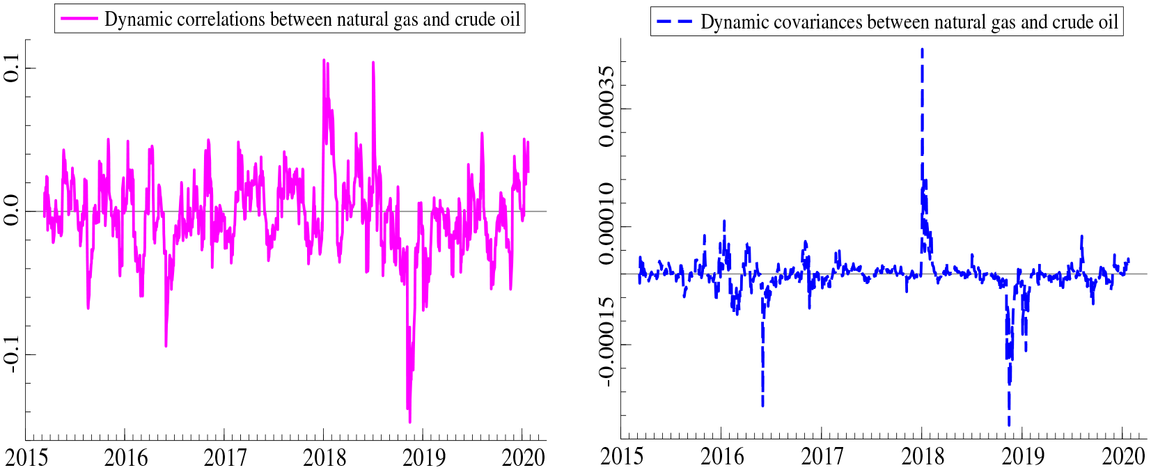
Dynamic correlations and covariances between natural gas and crude oil
To make the CAViaR approach even more realistic on the financial side, we consider both short and long trading positions of energy market investors. Our VaR results reveal considerably good performance, in particular, for the long trading positions. Intuitively, when investors take long positions, their “downside” risk exposure “hits” due to sharp price declines do not exceed those captured by our VaR forecasts. In other words, our volatility model is rather appropriate such that empirical VaR forecasts (hits) inferred from it are statistically similar to the expected VaR α levels. In contrast, the reverse mechanism (i.e, short trading position) does not generate very accurate forecasts, especially when the risk tolerance is considered as extremely low (i.e., at the quantile of 99% and above). One possible explanation could be related to the asymmetric nature between “extreme” left and “extreme” right tail behavior of return distributions. For quantiles of 95%, our empirical VaR forecasts based on short trading positions are, once again, in line with the expected values (with the p-value around 0.753), revealing good detection (hitting) performance. These VaR results are unreported for brevity, but they are available upon request. We thank the anonymous referee for this suggestion.
The right panel of Figure 5 further shows the dynamic (daily) covariances between crude oil and gas. It is quite visible that covariance between crude oil and gas changes its sign over time and there are three distinct episodes in which covariance becomes relatively high. The covariance appears to be sharply negative in May 2016 and late 2019 whereas we observe a sudden upward increase in the beginning of 2018.
5.3 Predictive Models and Forecasting Results
This subsection will report the results of forecasting the conditional volatility of natural gas returns

where
Table 6 shows the statistical accuracy of competing models. Surprisingly, the AR(2) model fared well against sophisticated alternatives. The forecast gains from including conditional volatilities of crude oil, electricity and temperature returns are modest (below 3%). We note that the RF model demonstrated the lowest prediction errors, only slightly better than the FF-D-ANN model. Despite its recent popularity in machine learning, the XGB model performed poorly. In all, our findings suggest that forecasting natural gas volatility is an elusive goal that is potentially hindered by geopolitical shocks and multifractality in natural gas markets (Lv and Shan, 2013).
Comparison of predictive models for conditional volatility
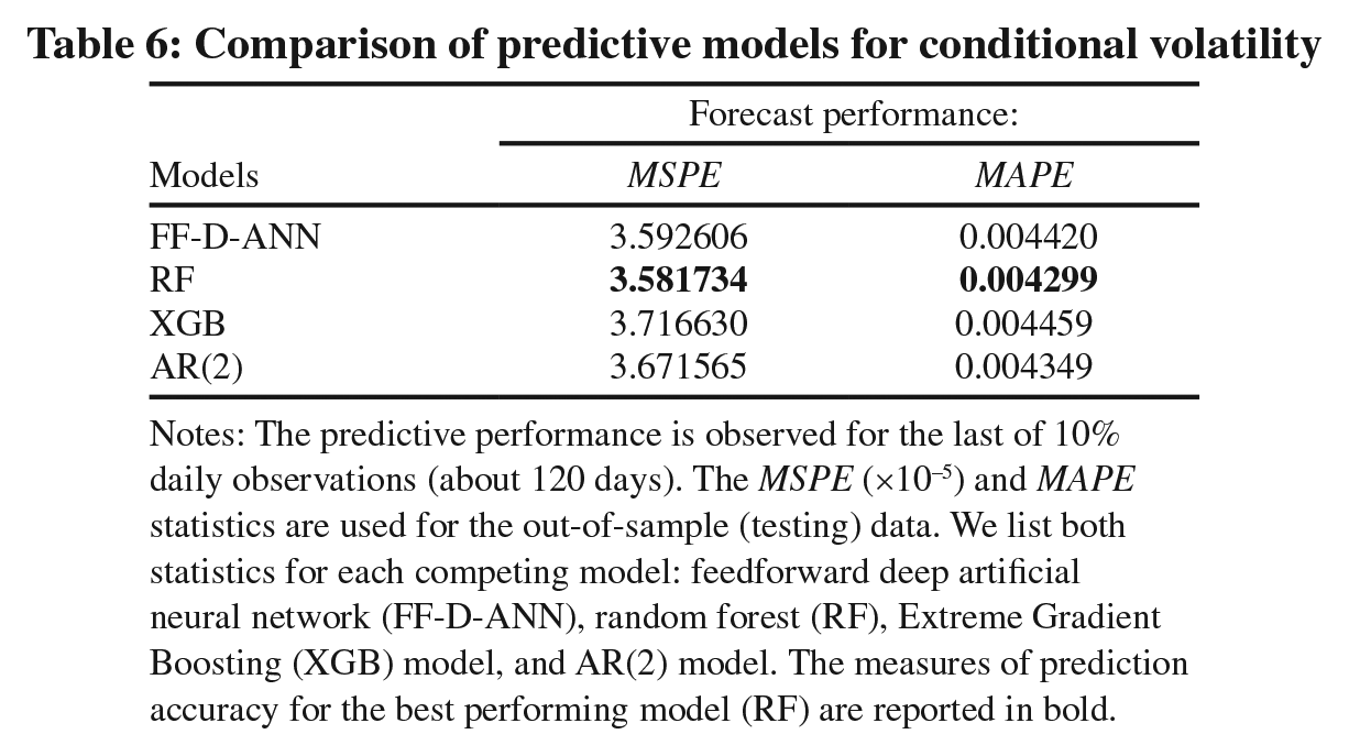
Notes: The predictive performance is observed for the last of 10% daily observations (about 120 days). The MSPE (×10−5) and MAPE statistics are used for the out-of-sample (testing) data. We list both statistics for each competing model: feedforward deep artificial neural network (FF-D-ANN), random forest (RF), Extreme Gradient Boosting (XGB) model, and AR(2) model. The measures of prediction accuracy for the best performing model (RF) are reported in bold.
To understand the relative contribution of input features and their role in volatility forecasting, as we did in Table 4, we turn to the XAI methods next. Table 7 lists the SHAP (column 2) and Gini (column 3) values for the estimated RF model. Both methods emphasize the importance of volatility dynamics and long memory
19
in the natural gas market, with both lags—
Relative contribution of volatility predictors
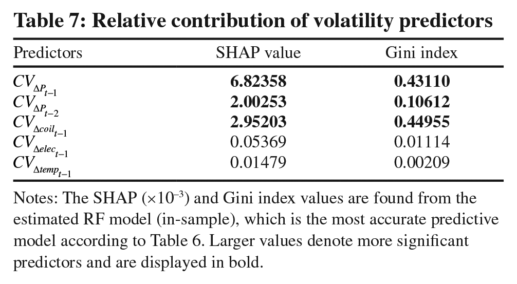
Notes: The SHAP (×10−3) and Gini index values are found from the estimated RF model (in-sample), which is the most accurate predictive model according to Table 6. Larger values denote more significant predictors and are displayed in bold.
6. Predictability during covid-19 and russia-ukraine crisis
This section tests alternative model specifications for both the U.S. and European natural gas markets on an updated data set that spans the January 1, 2020 to July 5, 2022 time period (approximately 640 daily observations). 20 It is worthwhile to note that, when compared to 2015–2020, the most recent time period was marked by higher volatility in the U.S. (COVID-19 pandemic) and extreme volatility in the E.U. in 2022 (Ukraine crisis). First, the forecasting model for the U.S. market is expanded to include a seasonal component as in Berrisch and Ziel (2022). Then, in the spirit of Berrisch and Ziel (2022). we define a non-linear one-day-ahead forecasting model for the E.U. gas returns as follows:

where ΔTTF is the change in the logarithm of daily TTF Hub natural gas price (ΔTTFt = ln(TTFt) – ln(TTFt–1)), Δelec is the logarithmic change of the German day-ahead peak power price, Δcoil is the logarithmic change of the one-month-ahead Brent crude oil futures price, Δtemp is the daily change of the average German temperature, Δeua is the logarithmic change of the spot price of the EUA, Δstorage is the logarithmic change of the European natural gas storage levels, and seas is a seasonal component computed as a one-week moving average in TTFt, lagged by one year.
Since we are especially interested in how agile the non-linear artificial intelligence (AI) models would be to adjust to market regime shifts (and the resulting excess volatility) during the 2020–2022 period, relative to the traditional linear model, in Table 8, we compare the return forecasts generated by the following models: feedforward deep artificial neural network (FF-D-ANN), random forest (RF), Extreme Gradient Boosting (XGB) model, and the linear model (LINEAR). Such analysis would shed light on whether the AI methods for natural gas forecasting may represent a viable approach to practitioners, considering their high implementation cost.
Comparison of predictive models for returns (2020–2022)
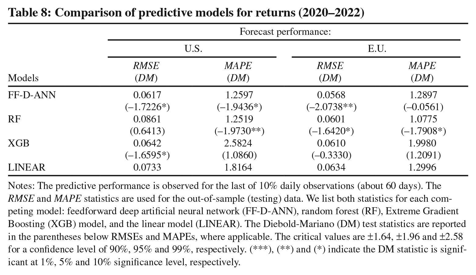
Notes: The predictive performance is observed for the last of 10% daily observations (about 60 days). The RMSE and MAPE statistics are used for the out-of-sample (testing) data. We list both statistics for each competing model: feedforward deep artificial neural network (FF-D-ANN), random forest (RF), Extreme Gradient Boosting (XGB) model, and the linear model (LINEAR). The Diebold-Mariano (DM) test statistics are reported in the parentheses below RMSEs and MAPEs, where applicable. The critical values are ±1.64, ±1.96 and ±2.58 for a confidence level of 90%, 95% and 99%, respectively. (***), (**) and (*) indicate the DM statistic is significant at 1%, 5% and 10% significance level, respectively.
As explained in subsection 2.1, the optimal FF-D-ANN model architecture for the E.U. model was obtained from the validation data as follows: “6-7-11-1”, i.e., two hidden layers with 7 and 11 neurons, respectively (with sigmoid activation functions). The optimal RF model structure (from the validation data) follows subsection 2.2, with 80–100 trees that form the forest. Similar settings were used for the XGB model: 80–120 trees with no restriction on the maximum depth of each tree.
Table 8 reveals that for both the U.S. and the E.U. markets non-linear models deliver statistically significant forecast improvements as measured by the Diebold and Mariano (1995) (DM) test statistic. 21 Specifically, the RF and the FF-D-ANN models forecast natural gas returns better than the linear model for most of the performance metrics. For the U.S. (E.U.), the FF-D-ANN model produces an improvement of 16% (11%) based on the root-mean-squared prediction error (RMSE) and it is statistically significant at the 10% (5%) significance level. The forecast improvements in the MAPE generated by the RF model range from 17% (E.U.) to 31% (U.S.). This leads to the conclusion that the extreme volatility observed in the E.U. in early 2022 somewhat diminished the forecast gains from non-linear models, but they were still substantially more accurate than that from the linear model. The XGB model did not exhibit any consistent forecast accuracy during the 2020–2022 time period. In comparison to our analysis in Section 4, the results presented in Table 8 demonstrate predictive usefulness and adaptability of AI models when markets experience structural breaks and increased volatility. 22
Table 9 displays the SHAP values for each predictor of the best-performing U.S. and E.U. models in terms of the RMSE (i.e., the FF-D-ANN model). The electricity price emerges as the most dominant predictor in both markets, while the crude oil price seems to have lost its predictive power. Clearly, the decoupling of oil and natural gas prices depicted in Figure 4 that commenced in late 2017 has permeated over the past few years. Also, the results support the inclusion of the seasonal component that is important for forecasting both Henry Hub and TTF Hub returns. Finally, the non-linear effect of the EUA spot price (Δeua) is the third most important for predicting ΔTTF fluctuations. These findings complement Berrisch and Ziel (2022) in that they found the effect of Δeua to be significantly positive in the one-day-ahead ΔTTF forecasting. 23 They also conjectured the existence of unexploited non-linear dependencies originating in Δeua and seas, for which we provide empirical evidence.
Relative contribution of predictors for returns (2020–2022)
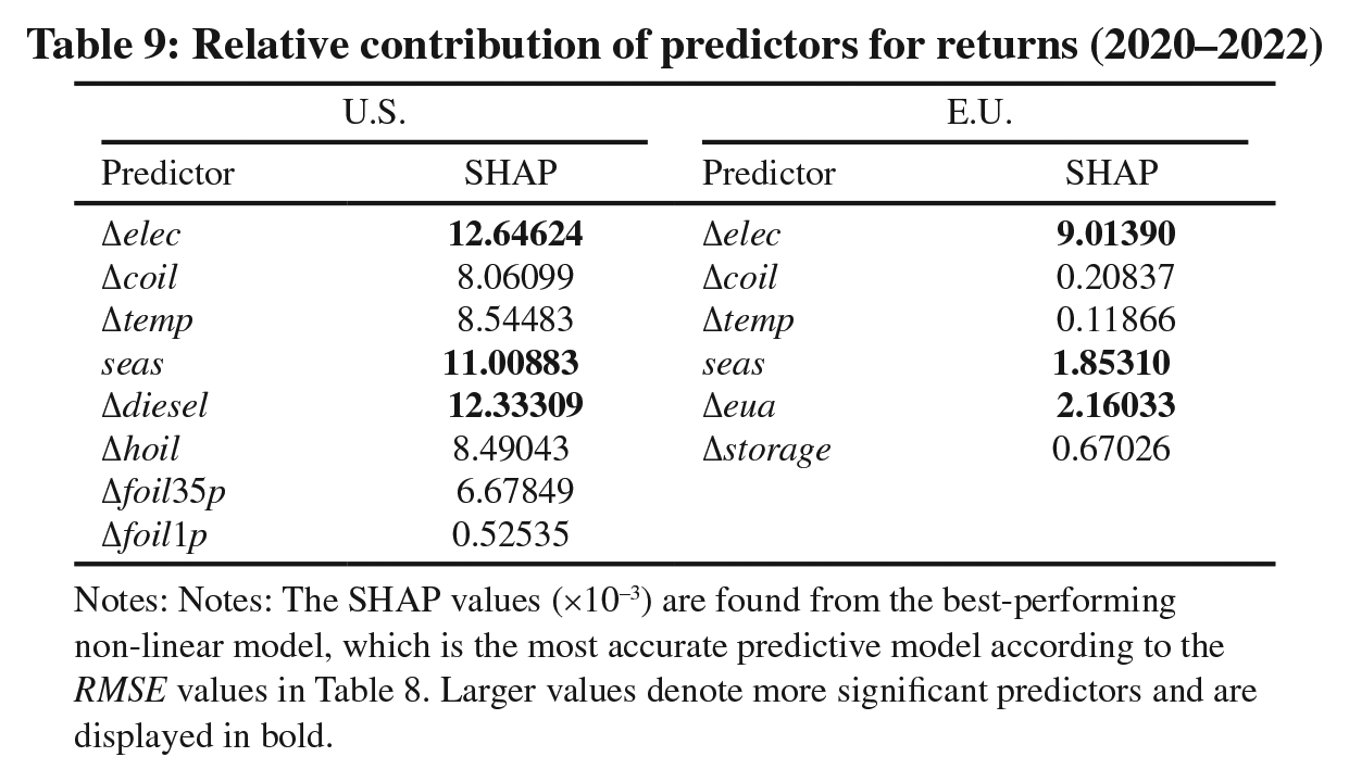
Notes: Notes: The SHAP values (×10−3) are found from the best-performing non-linear model, which is the most accurate predictive model according to the RMSE values in Table 8. Larger values denote more significant predictors and are displayed in bold.
We focus on the conditional volatility of natural gas returns and the corresponding predictors next. We follow the same approach as in Equation 13, with the inclusion of the seasonal component. The results of our predictive exercises are listed in Table 10. There are several notable findings that warrant attention. First, all non-linear models performed remarkably well for the U.S. market and their out-of-sample forecasts are statistically significantly (at the 1% significance level) more accurate than those of the linear model. The forecast improvements in the RMSE (MAPE) range from 42% to 74% (57% to 78%). We can conclude that high volatility that characterized the U.S. natural gas market during the 2020–2022 period was to a large degree predictable with the AI methods, while the linear model faced considerable difficulties adapting to structural breaks. Then, the E.U. market reveals a different story, with only the FF-D-ANN model performing consistently well in forecasting the conditional volatility of natural gas returns. It appears that in comparison to decision tree models such as RF and XGB, sophisticated deep learning models provide better adaptability in the presence of extreme market volatility. 24
Comparison of predictive models for conditional volatility (2020–2022)
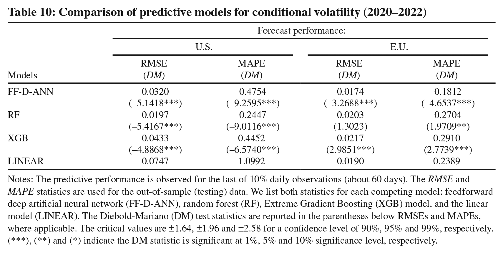
Notes: The predictive performance is observed for the last of 10% daily observations (about 60 days). The RMSE and MAPE statistics are used for the out-of-sample (testing) data. We list both statistics for each competing model: feedforward deep artificial neural network (FF-D-ANN), random forest (RF), Extreme Gradient Boosting (XGB) model, and the linear model (LINEAR). The Diebold-Mariano (DM) test statistics are reported in the parentheses below RMSEs and MAPEs, where applicable. The critical values are ±1.64, ±1.96 and ±2.58 for a confidence level of 90%, 95% and 99%, respectively. (***), (**) and (*) indicate the DM statistic is significant at 1%, 5% and 10% significance level, respectively.
To explore the relative usefulness of predictors in forecasting conditional volatility of gas returns in the U.S. and E.U. markets (2020–2022), we perform the SHAP analysis similar to that in Table 7. From Table 11, we find that the conditional volatility of electricity returns, and the conditional volatility of diesel and fuel oil returns are most informative for predicting the conditional volatility of gas returns in the U.S. market. On the other hand, the most important predictor for the conditional volatility of gas returns in the E.U. market is the conditional volatility of EUA returns. This shows that CVΔeua significantly impacted the coal-to-gas switching cost and thus gas demand when extreme market volatility hit the E.U. over the 2020–2022 period.
Relative contribution of predictors for volatility (2020–2022)
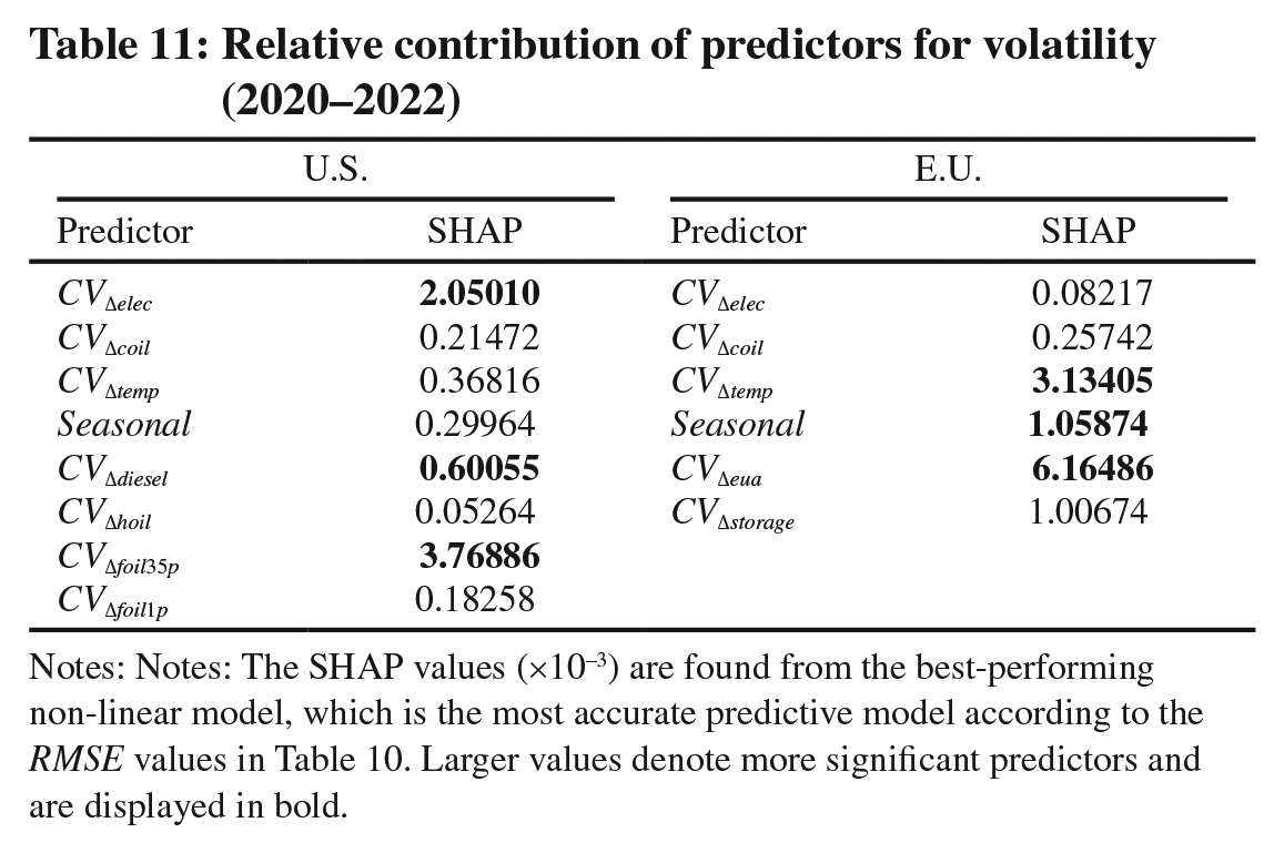
Notes: Notes: The SHAP values (×10−3) are found from the best-performing non-linear model, which is the most accurate predictive model according to the RMSE values in Table 10. Larger values denote more significant predictors and are displayed in bold.
To further gauge the forecast ability of the competing models, next, we perform the ranking analysis using the model confidence set (MCS) by Hansen et al. (2011). Table 12 contains MCS p-values and model rankings for returns forecasting with respect to two loss functions: the squared error (SE) and the absolute error (AE). Clearly, the results are in accord with those from Table 8 and show that the FF-D-ANN model consistently outperforms the competing methods in both markets. 25 It is statistically significantly ranked first across the two loss functions and natural gas markets, while the linear model is ranked last or second last.
MCS for linear and non-linear return forecasts (2020–2022)
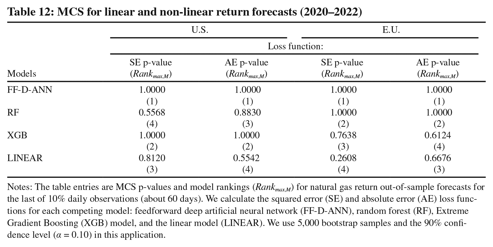
Notes: The table entries are MCS p-values and model rankings (Rankmax,M) for natural gas return out-of-sample forecasts for the last of 10% daily observations (about 60 days). We calculate the squared error (SE) and absolute error (AE) loss functions for each competing model: feedforward deep artificial neural network (FF-D-ANN), random forest (RF), Extreme Gradient Boosting (XGB) model, and the linear model (LINEAR). We use 5,000 bootstrap samples and the 90% confidence level (α = 0.10) in this application.
As for the volatility forecasting, Table 13 reveals slightly more complex rankings that do not show a clear dominance of a single model. Nevertheless, non-linear AI methods (FF-D-ANN and RF) are robustly more accurate than the linear model across the SE, the AE, and the Gaussian likelihood (QLIKE) loss functions. For the majority of the cases, the linear model is statistically excluded from the rankings due to its poor performance. Such findings essentially mirror the evidence from Table 10. 26
MCS for linear and non-linear volatility forecasts (2020–2022)
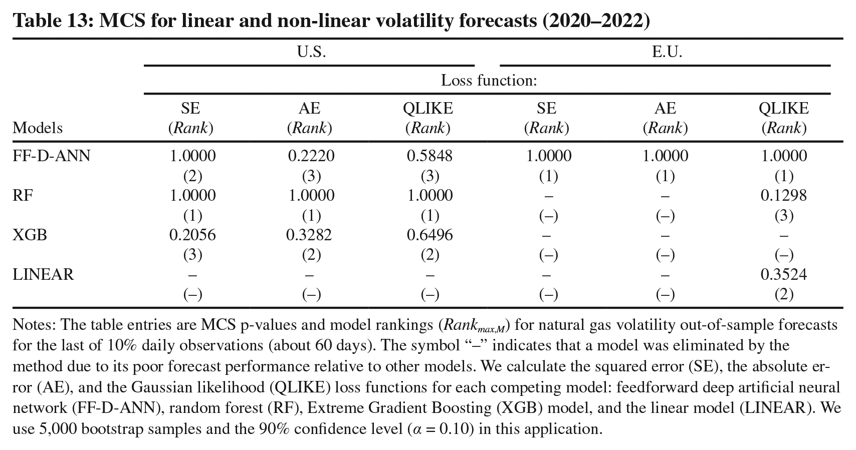
Notes: The table entries are MCS p-values and model rankings (Rankmax,M) for natural gas volatility out-of-sample forecasts for the last of 10% daily observations (about 60 days). The symbol “–” indicates that a model was eliminated by the method due to its poor forecast performance relative to other models. We calculate the squared error (SE), the absolute error (AE), and the Gaussian likelihood (QLIKE) loss functions for each competing model: feedforward deep artificial neural network (FF-D-ANN), random forest (RF), Extreme Gradient Boosting (XGB) model, and the linear model (LINEAR). We use 5,000 bootstrap samples and the 90% confidence level (α = 0.10) in this application.
7. Conclusions: Explainable Non-Linearities
Forecasting natural gas prices and volatility at day-ahead horizons poses a major research challenge. While traditional wisdom has been to rely on the oil-indexed formula (e.g., in Central Europe and Asia), the interaction between demand and supply forces has been the primary driver of gas prices in the U.K. and the U.S. It is unclear, however, whether it would be possible to combine factors related to the oil-indexed formula with other potential gas price predictors such as electricity price and temperature. We propose a two-stage strategy to, first, forecast natural gas price returns as well as volatility and, then, to quantify and interpret the model predictors. In the first stage, we run sophisticated non-parametric models based on machine learning and demonstrate their forecast superiority relative to a barrage of alternative model specifications. We also find that the linear model and its variants (RIDGE, LASSO, and ELASTIC) are inaccurate and perform no better than a random walk. Our robust XAI analysis pins down the most important non-linear predictors of the Henry Hub spot price movements over the 2015–2020 period, namely crude oil price, electricity price, and temperature. Even though the findings emphasize the time-varying complexity of relationships, the model shows that crude oil and electricity act as important drivers for natural gas. We provide compelling evidence that the oil-indexed formula suffers from an omitted variable bias and is an imperfect approximation of natural gas price dynamics. Volatility forecasting, however, presents additional difficulties where the informativeness of temperature- and electricity-related predictors vanishes from the model. Our results highlight the ubiquitous role of crude oil in forecasting both natural gas returns and volatility as well as the complex non-linear and dynamic nature of such interactions.
In addition to these insights and assessments, we further examine the predictive performance of the models during periods of high uncertainty (i.e., 2020–2022), and explore in particular the impact of the COVID-19 pandemic and the Russia-Ukraine crisis. In these periods when sharp structural breaks and extreme volatility grip the markets, we show that deep learning models provide better adaptability and lead to statistically significantly dominant forecast performance.
Our future research efforts will concentrate on linking gas prices and volatility to new prospective predictors. Given that geopolitical and pandemic uncertainties have caused recent excessive volatility episodes in gas prices, it would be sensible to quantify such forces into a global natural gas market ‘fear indicator’ that, for example, might be based on the implied volatility of natural gas option contracts. 27 Theoretically speaking, option prices are forward-looking and represent discounted expectations of future outcomes of the underlying price. Consequently, a stress indicator that is calculated from options could potentially serve as a useful gauge of gas price fluctuations. Furthermore, recent scholarly work suggests that carbon risk factors can explain part of the cross-sectional variation of stock returns (Oestreich and Tsiakas, 2015). Considering that a natural gas turbine produces about 30% (50%) less CO2 per MWh of electricity than a fuel oil (coal)-fired generating station, it would be natural to empirically explore the non-linear interplay between carbon price, natural gas price, oil price, electricity price and stock prices. In light of the findings of Prokopczuk et al. (2021), such interactions can be further mapped into a trading strategy, particularly by utilizing intraday data, or an in-depth VaR-type assessment for measuring extreme risk exposures. Last but not least, understanding the carbon price and volatility dynamics in both time and frequency domains, driven by the relative importance of various factors, might deliver valuable lessons about the effectiveness of particular carbon policies.

Supplemental Material
sj-pdf-1-enj-10.5547_01956574241277302 – Supplemental material for Drilling Deeper: Non-Linear, Non-Parametric Natural Gas Price and Volatility Forecasting
Supplemental material, sj-pdf-1-enj-10.5547_01956574241277302 for Drilling Deeper: Non-Linear, Non-Parametric Natural Gas Price and Volatility Forecasting by Dusan Bajatovic, Deniz Erdemlioglu and Nikola Gradojevic in The Energy Journal
Footnotes
1.
Recent studies indicate the rising role of alternative pricing mechanisms, next to oil-indexation, or the so-called “oil price escalation” (OPE). Among those works, the “gas-on-gas competition” (GOG) appears to stand out, as a market-based hub pricing through which market competitively determines the price of natural gas by demand and supply. New forms of arrangements become more favorable, particularly for the buyer-side. Indexation-based pricing, however, has lost its attractiveness at the global level: more countries continue to adopt the new GOG mechanism, while oil-indexation has been steadily diminishing. For example, Till and McHich (2020) show that there are about 14 countries using the GOG in 2012 whereas this number increased to 34 in 2019. For an in depth discussion on the relevance of oil-indexation and alternative contract mechanisms, see e.g., Till and McHich (2020) and ![]() .
.
2.
Considering that the majority of our predictors will be prices that are presumably non-stationary processes, log differencing is necessary to achieve stationarity. We demonstrate this on our data set in Section 3.
3.
5.
Other studies on the predictability of natural gas prices include Gaillard et al. (2016) and Wang et al. (2020a), among others. See also Mirantes et al. (2012), who characterize the seasonality in natural gas prices. ![]() further examine the hedging implications of size risk with a particular focus on the U.S. gas market.
further examine the hedging implications of size risk with a particular focus on the U.S. gas market.
6.
See Zhang et al. (2015) for a related discussion. ![]() further argue that the relationship between natural gas prices and electricity prices is in fact bi-directional. On the one hand, higher gas prices could translate into higher electric power generation costs that may be borne by electricity consumers. On the other hand, higher demand for electricity (e.g., due to extremely hot weather) would increase electricity prices and that may translate into higher demand for natural gas (and higher gas prices).
further argue that the relationship between natural gas prices and electricity prices is in fact bi-directional. On the one hand, higher gas prices could translate into higher electric power generation costs that may be borne by electricity consumers. On the other hand, higher demand for electricity (e.g., due to extremely hot weather) would increase electricity prices and that may translate into higher demand for natural gas (and higher gas prices).
7.
We do not empirically restrict the maximum depth of the tree, because we find that the RF model’s forecast performance is not sensitive to reasonable choices such as 10 or 20 levels.
8.
The sample ends prior to the COVID-19 pandemic. Hence, the impact of potential structural breaks on our results is minimal.
9.
As is standard, we perform unit root tests on all variables. For the majority of cases, the null hypothesis of non-stationarity is not rejected at the 1% significance level and the first difference transform had to be applied to achieve stationarity. These test results are unreported for brevity, but they are available upon request.
10.
The linear regression was run with robust standard errors. We did not detect any significant multicollinearity problems with regressors. The average VIF was around 4 and no larger than 8 for any regressor. An alternative regression setting with lagged regressors is even more misspecified where the only statistically significant parameter was β7 (Δelect+1).
12.
For further insights on out-of-sample forecasting of commodity prices, see e.g., Wang et al. (2020b) and ![]() .
.
13.
In this line of research, see Mu (2007) and ![]() , who explore the impact of weather shocks and demand shocks on natural gas volatility, respectively.
, who explore the impact of weather shocks and demand shocks on natural gas volatility, respectively.
14.
We obtain strong convergence using numerical derivatives based on the Broyden-Fletcher-Goldfarb-Shanno (BFGS) algorithm as our estimation method.
15.
The estimated coefficient of GARCH is negative, but this is due to the FIEGARCH specification and we confirm that conditional variance is still positive. By estimating a GARCH model rather than a FIEGARCH specification, we further assessed this particular case and found that the estimated coefficient (based on the estimated standard GARCH model) is statistically significant with positive sign. These results are available upon request.
16.
This result holds even if we use the volatility of explanatory variables in the variance equation, rather than returns. Further, our findings remain unchanged when we use only electricity as a single explanatory variable. It is also worth mentioning that the estimation of FIAPARCH model reveals no evidence for asymmetric (negative vs. positive) effects of returns on volatility, which in turn confirms that there is no asymmetric (sign) effect.
17.
From a risk management perspective, it is of interest to conduct a value-at-risk (VaR) analysis based on our underlying conditional volatility model. For this purpose, we adopt the dynamic, “conditional autoregressive VaR (CAViaR) approach” of ![]() and test the accuracy of our VaR forecasts accordingly. This specific VaR measurement approach relies on non-linear regressions (with respect to parameters) and hence it is compatible with our framework.
and test the accuracy of our VaR forecasts accordingly. This specific VaR measurement approach relies on non-linear regressions (with respect to parameters) and hence it is compatible with our framework.
18.
To assess the statistical significance of our estimated dynamic correlations properly, we further performed a formal statistical test. Our results indicate a very low uncertainty around the mean correlations and, also, that the mean value of estimated correlations is statistically different from zero. Moreover, as we focus more on the significance of each (i.e., single, daily) estimated correlation value, we identify a very small fraction of daily correlations that are within this range. These results are unreported for brevity, but they are available upon request.
20.
We are thankful to the three anonymous Referees for their thoughtful and constructive comments, which have substantially improved the paper. We are also grateful to Professor James L. Smith, Professor Adonis Yatchew, and Mr. David Williams for the valuable feedback. Luka Vulicevic provided some excellent research assistance.
21.
The DM test is used to test the null hypothesis that there is no difference in the RMSE and MAPE of two alternative forecasting models. It is asymptotically distributed as a N(0,1).
22.
It is perhaps worth mentioning that, by definition, the RMSE is more sensitive to outliers than the MAPE (i.e., it penalizes extreme forecast errors more), but it is an unbiased measure. This is the likely reason for the differences in performance. However, they are both statistical measures, not economic measures that a practitioner would need to consider for trading decisions. We believe a practitioner should first rely on directional forecasts (that we leave for future research), then the RMSE, followed by the MAPE.
23.
In unreported results, based on a heatmap plot (available upon request), we document a mostly positive non-linear relationship between Δeua and ΔTTF as well. This can be interpreted as a situation where positive Δeua make power generation by using natural gas more attractive (than by using coal) and ΔTTF becomes positive.
24.
The predictive performance of models remained unchanged even after we had controlled for several volatility dummy variables: 1) COVID-19 period, 2) Ukraine crisis period, 3) COVID-19 and the Ukraine crisis combined, 4) “high uncertainty shocks” in the E.U. between 2020–2022 (this dummy controls for turbulent market conditions), and 5) “low uncertainty shocks” in the E.U. between 2020–2022 (this dummy controls for calm market conditions). Moreover, it is worth stressing that ![]() shows no DM sign switching across indicators (MAPE, RMSE) but still across markets (US, EU). Only the FF-D-ANN performs robustly better than the linear model across markets and indicators and does so for both returns and volatility forecasts.
shows no DM sign switching across indicators (MAPE, RMSE) but still across markets (US, EU). Only the FF-D-ANN performs robustly better than the linear model across markets and indicators and does so for both returns and volatility forecasts.
25.
26.
It is worth emphasizing that complex non-linear models may fare less well than a simple linear model. This shows that the latter is not nested in the former. More importantly, on the trading side, models deployed for actual trading must be robust and more complex (and hence harder to program, check and maintain), and they must perform significantly and robustly better than simpler alternatives.
27.
As a point of comparison, in equity markets, the VIX is an index providing theoretical 30-day market expectations based on option contracts written on the S&P 500 Index. The VIX indicates the level of fear (or stress) in the stock market and is often referred to a the ‘fear index’. Similar risk indicators have been devised in Gradojevic (2021) and ![]() .
.
References
Supplementary Material
Please find the following supplemental material available below.
For Open Access articles published under a Creative Commons License, all supplemental material carries the same license as the article it is associated with.
For non-Open Access articles published, all supplemental material carries a non-exclusive license, and permission requests for re-use of supplemental material or any part of supplemental material shall be sent directly to the copyright owner as specified in the copyright notice associated with the article.