Outsourcing Strategy of E-waste Collection Activity for a Manufacturer

Abstract

A pair of mixed integer linear programming model is developed for manufacturers to formulate e-waste collection outsourcing strategy in India. The pair consists of single and multi-period decision models for manufacturer to choose from based on their requirement.

Keywords

E-waste collection outsourcing strategy Indian electronic products manufacturer

Introduction and Motivation

The E-waste (Management and Handling) Act, 2012 mandates a manufacturer to engage in collection of e-waste activity in-house or outsource to independent collection firms (ICFs). Past literature on the collection activity outsourcing strategy was limited to collection of used products by a single collection firm in single period context (Atasu, Toktay, & Van Wassenhove, 2013; Savaskan, Bhattacharya, & Van Wassenhove, 2004).

In real-life situation, a number of potential independent firms are available at various locations to the manufacturer, to perform e-waste collection at dissimilar transfer prices. The quantity of the e-waste delivered to a collection firm is uncertain but can be estimated. The e-waste is disposed by consumers in multiple periods. Under these conditions, a manufacturer has to optimally select ICFs and in-house collection facility for performing e-waste collection for minimizing costs.

Model Formulation

In this paper, for the e-waste collection strategy problem of a manufacturer, a single period mixed integer linear programming (MILP) model is formulated, which is extended to multi-period context. Following assumptions are made for developing the mathematical models to realize the research objectives.

There is huge demand for the remanufactured products in India and all the recovered products in a period can be sold in the same period (Mitra, 2007; Ordoobadi, 2009; Srivastava & Srivastava, 2006).

Customers return products only on completion of the service life of products (Kushwaha & Bhattacharya, 2015).

The quantity of e-waste likely to be received at a potential collection centre can be estimated (Martin et al., 2010; Ordoobadi, 2009; Ovchinnikov et al., 2014).

For a single period situation production, use and product return occur in same period.

A product is consisting of several types of subassemblies. A product consists of exactly one subassembly of each type (Abbey, Guide, & Souza, 2013; Ordoobadi, 2009).

The e-wastes are disassembled, the subassemblies with acceptable service life are inventoried and remaining is disposed off (Ordoobadi, 2009).

The products will be remanufactured using inventoried recovered subassemblies only (Abbey et al., 2013; Ordoobadi, 2009).

Customers who are likely to return e-waste to a potential collection centre which is not authorized will return the products to the manufacturer (Acer, n.d.; Dell, n.d.; Samsung, n.d.).

The subassemblies which are left out at end of finite planning period will be disposed off at a salvage value (Ordoobadi, 2009).

For a finite planning period model if an independent firm is selected at the beginning of the first period, it will be authorized and will remain selected for remaining periods (Ovchinnikov et al., 2014).

The manufacturer has one facility to perform reverse supply chain activities (Atasu et al., 2013; Ordoobadi, 2009; Ovchinnikov et al., 2014; Savaskan et al., 2004).

Only outsourcing of e-waste collection activity to potential ICFs are considered. The manufacturer will remanufacture and remarket the recovered products. Hence, the objective of the manufacturer could be cost minimization as the revenue is fixed.

The total cost of e-waste collection consist of the fixed cost and total variable cost involved in collection of used products by manufacturer, and the total transfer fee paid to selected ICFs (notations are given in Appendix 1):

Z = F_{A 0} D_{A 0} + ​ \sum^{​} ​ A_{0 i} X_{i}^{1} + ​ \sum^{​} ​ A_{i} X_{i}^{1}

(1)

First and second terms are the fixed and the variable cost incurred by manufacturer for collection of e-waste. The third term is the total transfer fee paid to the ICFs.

Constraints: The constraints are:

\sum^{​} ​ X_{i}^{1} = ​ α p_{1}

(2)

X_{i}^{1} = �_{i} α p_{t - r} D_{A i} \forall i = 1, 2, . . ., I

(3)

X_{0 i}^{1} = ε_{i} α p_{t - r} (1 - D ​_{A i}) \forall i = 1, 2, . . ., I

(4)

X_{0}^{1} \leq 2 p_{1} D ​_{A 0}

(5)

X_{i}^{1} \geq 0 \forall i = 0, 1, 2, . . ., I

(6)

D ​_{A i} \in {0, 1} \forall ​ i = 0, 1, 2, . . ., I

(7)

Constraint (2) ensures that all available product returns are received by manufacturer and the ICFs. Constraint (3) makes sure that an ICF receives the estimated number of product returns only if selected and authorized. Quantity of used products received by manufacturer from individual region where an ICF is not selected is given by Constraint (4). Constraint (5) implies that the manufacturer engages in collection activity only if the product returns are received. The RHS gives an upper bound on the product returns received by the manufacturer. Constraint (6) enforces non-negativity of decision variables. Constraint (7) imposes binary constraint on decision variable for selection and authorization of ICF. The cost function Z is to be minimized subjected to Constraints (2) to (7).

The single period model is further extended to multi-period model. The total costs is the summation of fixed cost incurred by manufacturer in setting up used product collection facility and variable costs of performing reverse supply chain activities. The discounted costs function for the planning period is:

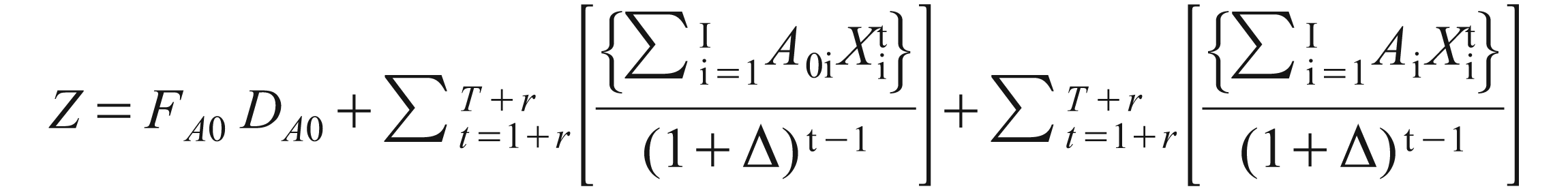
Z = F ​_{A 0} D ​_{A 0} + \sum^{​} ​ [\frac{{\sum^{​} ​ A_{0 i} X_{i}^{t}}}{{(1 + Δ)}^{t - 1}}] + \sum^{​} ​ [\frac{{\sum^{​} ​ A_{i} X_{i}^{t}}}{{(1 + Δ)}^{t - 1}}]

(8)

First term on RHS of (8) is the fixed cost incurred by manufacturer and the second and third terms are variable costs incurred for used product collection by the manufacturer and ICFs.

Constraints: The constraints are:

\sum^{​} ​ ​ X_{i}^{t} = α p_{t - r} \forall t = 1, . . ., T + r

(9)

X_{i}^{t} = ε_{i} α p_{t - r} D ​_{A i} \forall i = 1, 2, . . ., I a n d \forall t = 1, 2, . . ., T + r

(10)

X_{0 i}^{t} = ε_{i} α p_{t - r} (1 - D ​_{A i}) \forall i = 1, 2, . . ., I a n d \forall t = 1, 2, . . ., T + r

(11)

X_{0}^{t} \leq \sum^{​} ​ p_{t - r} D ​_{A 0} \forall t = 1 + r, . . ., T + r

(12)

X_{i}^{t} \geq 0 \forall i = 0, 1, 2, . . ., I a n d \forall t = 1, 2, . . ., T + r

(13)

D ​_{A i} \in {0, 1} \forall i = 0, 1, 2 . . ., ​ I

(14)

Constraints (9) through (14) are multi-period extensions of Constraints (2) through (7). The objective function Z is to be minimized subjected to Constraints (9) to (14).

Solution Approach

The models developed come under the category of MILP. The branch and bound algorithms available in the software LINDO could be used to arrive at a solution.

The parameter values can be chosen after literature review and conducting case studies for e-waste collection for some selected products like batteries, televisions, laptops and mobile phone handsets. Sensitivity analysis using the formulated models is to be used for examining the sensitivity of the solution to changes in the parameter values.

Contribution

Manufacturers in India would be able to formulate optimal outsourcing strategy for e-waste collection. The development of multi-period outsourcing decision models for manufacturers is contribution of the study to OEMs (original equipments manufacturers) and other manufacturing firms.

Appendix 1: Notations

Indices

i: Index of potential firm for collection of used products, = 1 ... I

t: Index of time period, = 1 ... T, for the single period model T = 1

s: Index of subassembly in the product, = 1 ... S

Parameters

r: Lead time between sales and return of e-waste, considered as constant in multi-period context. Note that in a single period context, it is assumed the used products are returned in the same period as that of production.

P_t: Quantity of new products produced by manufacturer in period t; t = 1, 2, . . ., T.

α: Fraction of new products produced in time period t which are returned in period t + r; t = 1, 2, . . ., T.

β_s: Fraction of subassembly type s in the total returned products which have acceptable service life for recovery and inventoried for reassembly.

F_A₀: Fixed cost incurred by manufacturer for engaging in collection of used products at the beginning of the planning period.

A_0i: Per unit variable cost of e-waste collection incurred by manufacturer from ICF i.

A_i: Per unit variable cost paid by manufacturer to authorized ICF i for collecting product returns and supplying to manufacturer, i = 1, 2, . . ., I.

ε_i: Estimated fraction of total product returns likely to be received by potential ICFi; $i = 1, 2 . . . I; \sum^{} ε_{i} \leq 1$ .

Δ: Rate of discount for calculating discounted cost.

Decision Variables

$X_{0}^{t}$ : Quantity of used products received by the manufacturer in the period t. For single period context t = 1. For multi-period context t = 1 + r, 2 + r, …, T + r.

$X_{0 i}^{t}$ : Quantity of used products received by the manufacturer directly from consumer in vicinity of ICF i in the period t. For single period context t = 1. For multi-period context t = 1 + r, 2 + r, …, T + r.

$X_{i}^{t}$ : Estimated quantity of used product returns at potential ICF i in the period t. For single period context t = 1. For multi-period context t = 1 + r, 2 + r, …, T + r.

D_A₀: A binary variable

= 1 if manufacturer is engaged in collection of used product

= 0, otherwise.

D_Ai: Binary variables, i = 1, 2, . . ., I

= 1 if a potential ICF i is selected and authorized for used product collection

= 0, otherwise.

References

Abbey

J. D.

, Guide

V. D. R.

, & Souza

G. C.

(2013). Delayed Differentiation for Multiple Lifecycle Products. Production and Operations Management, 22(3), 588–602.

Acer (n.d.). Acer India-eWaste Program-Recycle your old technology Acer computer and help protect environment. Retrieved November 13, 2014, from http://www2.acer.co.in/ewaste/Index.htm

Atasu

, Toktay

L. B.

, & Van Wassenhove

L. N.

(2013). How Collection Cost Structure Drives a Manufacturer’s Reverse Channel Choice. Production and Operations Management, 22(5), 1089–1102

Dell (n.d.), Recycling-Frequently acked questions, Retrived February 19, 2015 from http://www.dell.com/learn/in/en/incorp1/corp-comm/recycling-faq-apj-in?c=in&l=en&s=corp&cs=incorp1

Kushwaha

& Bhattacharya

(2015). Impact of cannibalization on product return under different demand scenarios. IUP Journal of Operations Management. 14(1), 39–53.

Martin

, Guide Jr., R

V. D.

., & Craighead

C. W.

(2010). Supply Chain Sourcing in Remanufacturing Operations: An Empirical Investigation of Remake Versus Buy. Decision Sciences, 41(2), 301–324.

Mitra

(2007). Revenue management for remanufactured products. Omega, 35(5), 553–562. doi:10.1016/j.omega.2005.10.003

Ordoobadi

S. M.

(2009). Outsourcing reverse logistics and remanufacturing functions: a conceptual strategic model. Management Research News, 32(9), 831–845.

Ovchinnikov

, Chao, & Xiang. (2014). Remanufacturing Strategies for OEMs without Remanufacturing Capabilities. Production and Operations Management.

10.

Samsung (n.d.) Samsung take back and recycling program, retriveed November 22, 2014 from http://www.samsung.com/in/samsungrecycle/

11.

Savaskan

R. C.

, Bhattacharya

, & Van Wassenhove

L. N.

(2004). Closed-Loop Supply Chain Models with Product Remanufacturing. Management Science, 50(2), 239–252.

12.

Srivastava

S. K.

, & Srivastava

R. K.

(2006). Managing product returns for reverse logistics. International Journal of Physical Distribution & Logistics Management, 36(7), 524–546.