
Abstract
This article reviews the different aspects involved in computational form finding of bending-active structures based on the dynamic relaxation technique. Dynamic relaxation has been applied to form-finding problems of bending-active structures in a number of references. Due to the complex nature of large spatial deformations of flexible beams, the implementation of suitable mechanical beam models in the dynamic relaxation algorithm is a non-trivial task. Type of discretization and underlying beam theory have been identified as key aspects for numerical implementations. References can be classified into two groups depending on the selected discretization: finite-difference-like and finite-element-like. The first group includes 3- and 4-degree-of-freedom implementations based on increasingly complex beam models. The second gathers 6-degree-of-freedom discretizations based on co-rotational three-dimensional Kirchhoff–Love beam elements and geometrically exact Reissner–Simo beam elements. After reviewing and comparing implementation details, the advantages and drawbacks of each group have been discussed, and open aspects for future work have been pointed out.
Keywords
Introduction
Bending-active structures are a kind of structures in which some members are pre-bent and then stabilized to achieve a certain desired configuration. The resulting system may reach considerable stiffness in relation to its weight due to the combination of the shape and slenderness of bent members and the post-bending stabilization by additional means as cables or membranes. The active bending principle has been used in vernacular architecture, for example, in the construction of tent-like dwellings (yurts or gers) by Asian nomadic peoples, where flexible timber slats are joined to form a lattice and bent to a cylindrical-shaped wall structure and a dome-shaped roof.
Since the construction of the Mannheim Multihalle 1 designed by Frei Otto, which is a pioneering modern application of the active bending principle in architecture, a number of dome-shaped grid-shells have been designed and built. Many of them have been designed as temporary or experimental structures as reported by Douthe et al., 2 Nicholas et al., 3 Pone et al. 4 or Harding et al. 5 The basic principle of grid-shells is the use of very flexible members which are joined and bent into a target shape and stabilized by fixing the ground supports in a convenient way. The result is a lightweight shell-like structure which is stiff enough due to its shape, but whose members are light and easy to manipulate during construction. The arrangement of joints and the length and stiffness of members allows for different overall shapes of the dome.
Bending-active structures are not limited to grid-shells; other realizations include small-scale grandstand roofs, 6 umbrellas and sculptural or ornamental applications. Lienhard et al. 7 have prepared a comprehensive review of this structural type.
The design process is non-trivial, and involves three stages: (1) determination of the initial shape (form finding), (2) determination of the initial stress state, and (3) modelling of the post-stabilization behaviour. Ideally, steps (1) and (2) are carried on simultaneously, as in the case of computational form finding of cable nets. Lienhard
8
compared governing variables in form-finding problems of form-active structures with variables in form finding of bending-active structures; he points out that in the former, the mechanical properties of the material are not governing the result, because shape is solely the result of equilibrium. As stated in this reference … the form finding of bending-active structures is largely influenced by the length of a beam […] that is bent as a result of the constraining boundary conditions as well as the mechanical behaviour of the beam or shell elements.
Therefore, the complex nature of the mechanical problem has led in some cases to design processes in which the shape is initially searched using physical models and afterwards the initial state is simulated by means of finite element models, in a so-called ‘integral approach’ to the design process. 8
Mainstream computational form-finding techniques rely on dynamic relaxation (DR) with different underlying mechanical models. From a numerical point of view, DR can be classified as an explicit method to find an equilibrium configuration. As suggested by D’Amico et al., 9 explicit methods are well suited to form-finding problems – for which tentative initial configurations may be far from equilibrium – in contrast with implicit solution methods, widely used in physical simulation of flexible structures under prescribed forces or displacements.
In addition to the pure form-finding problem, the need to solve the mechanical problem appears in the aforementioned steps (2) and (3). The second step may require tracking the full deformation path of the structural elements from an initial unstressed configuration. This usually involves traversing critical points in the equilibrium path, because the target configuration is a post-buckling state of the initial system. After the target shape has been reached and stabilized, the behaviour may not involve large displacements any more (unless the loads are again very large), but it is influenced by the inherited stress state. In this context, four basic features are required for a reliable simulation: (1) a sound mechanical model for flexible members undergoing large displacements of the reference lines and large rotations of the cross sections, and a numerical implementation capable of (2) traversing critical points in the equilibrium path, (3) allowing the addition and removal (in each stage) of certain members required to bring the system to the desired shape and/or stabilize it and (4) inheriting the stress state corresponding to a previous stage/configuration. Lienhard 8 has analysed two commercial finite element software packages and shown some drawbacks regarding features (2), (3) and (4) that lead to disregarding one of them and adapting and completing the other to meet these needs. In this reference, Lienhard proposes a form-finding procedure based on finite element simulations that start from undeformed/unstressed members and drive them to a target configuration by shortening notional elastic cables. This process has been recently improved using an isogeometric finite element implementation (Bauer et al. 10 ) that allows integration into a computer-aided design (CAD) environment (Bauer et al. 11 and Längst et al. 12 ).
Regarding the first mentioned requirement, the mechanical model, numerous references can be found in the context of finite element techniques. However, in the applications to bending-active structures, most attention has been directed to developing the geometry-related aspects of form finding, and to a lesser extent to the mechanics-related aspects. The following specific issues need be taken into consideration in the mechanical modelling of structures with bending-active members:
Large displacements and large rotations of member cross sections with respect to an initial configuration (generally not in equilibrium in a form-finding process) are to be expected.
Because active structures need to behave elastically in the target (bent) configuration – or equivalently, they should be far from yielding – active members are designed using materials with a high strength-to-Young’s modulus ratio and low-depth cross sections to reach high flexibility and resilience.
The previous observation implies that, in spite of displacements and rotations being large, strains will remain small in the target configuration.
Therefore, beam theories considering linear elastic material will be adequate to reproduce the behaviour of bending-active structures. The objectives of this work are to provide an overview of the mechanical models that have been used in computational form finding of bending-active structures and to review and classify the most relevant references with respect to this point of view. Only references in which explicit methods as DR are used for form finding will be considered, although as it has been mentioned before, other methods have also been used.
Key aspects in the specialization of flexible beam models for DR
It is assumed that the reader is familiar with the DR method to determine the equilibrium configuration of a mechanical system (refer, for example, to Barnes 13 ). The system to be analysed is discretized in a set of nodes. Fictitious masses are associated with model nodes. Stiffness relationships between nodes are defined. The analysis is started from an initial out-of-equilibrium configuration. Internal link forces corresponding to nodal positions at a given instant are calculated using stiffness relationships; external forces acting at nodes can be also introduced. With the resulting residual forces acting on every node, accelerations, velocities and displacements are evaluated. Artificial damping (or suppression of the kinetic energy) is used to bring the system to rest in static equilibrium.
The DR framework has been specialized to form finding of bending-active structures in different manners. The following aspects are tightly related and define the model specialization:
Type of discretization;
Underlying beam theory.
There are two types of discretizations in DR implementations reported in the literature: finite-difference-like discretizations and finite-element-like discretizations. In both cases, a key question is the way in which force–configuration relationships between nodes are established. Those relationships are determined in each case by the underlying beam theory, defined by the assumed kinematics, the selected elastic energy terms and the corresponding constitutive relations.
Beam theories for form finding of bending-active structures
Computational models for flexible rods rely on a suitable beam theory that models the three-dimensional (3D) deformation of the elastic body using a reduced set of kinematic and static variables. All examined references make use of the classical assumption of cross sections remaining plane and perpendicular to the deformed centreline of the rod, although with some differences between them. This assumption is a natural choice because strains induced by shear forces, which cause loss of planarity or perpendicularity of cross sections, are negligible in very slender members. The next sections review relevant aspects of the main beam theories in the context of form finding of bending-active structures. They are presented in order of increasing complexity; each theory may be considered a subset of the following one.
Euler–Bernoulli theory
The first reported solution for planar large deformations of a rod was developed by Euler in 1744, applying calculus of variations to the expression of the bending energy of the rod and assuming that (1) curvatures are proportional to bending moments – as suggested to him by Bernoulli – and (2) the rod length remains constant; this is equivalent to assuming inextensibility of the rod centreline and neglecting shear deformability. Conjugate variables in Euler–Bernoulli theory are centreline curvatures

and the deformation energy is given by
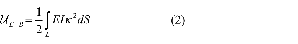
where

The configuration of a flexible rod under compressive loads applied at both ends deduced from this theory is called elastica. The linearized version of the curvature,
A refinement of Euler–Bernoulli theory can be obtained relaxing the inextensibility assumption. It involves the elongation energy
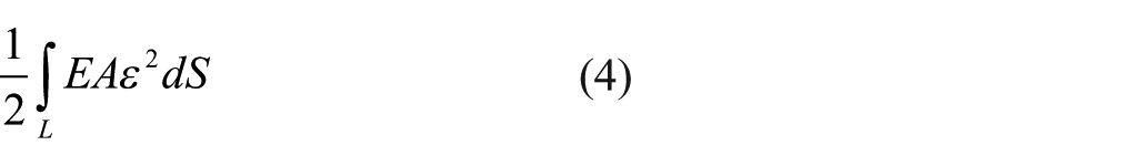
together with the constitutive relation between axial force and centreline strain

and the definition of the axial strain
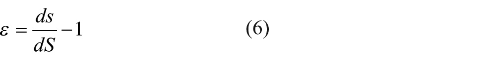
Non-linear solutions derived with this theory are called extensible elasticas. For the linear beam theory, equation (6) reduces to
Kirchhoff–Love theory
In 1859, Kirchhoff
14
proposed a 3D theory for very slender rods with extensible centreline that was developed by Love.
15
Kirchhoff–Love theory leads to negligible shear deformations, keeps Bernoulli’s moment-to-curvature proportionality in both principal axes and models torsion according to Saint–Venant’s theory (Dill
16
); it has been extensively used for developing finite elements for beams in the realm of small or moderately large displacements and rotations. Conjugate variables can be defined with respect to a set of orthogonal axes

and the deformation energy is
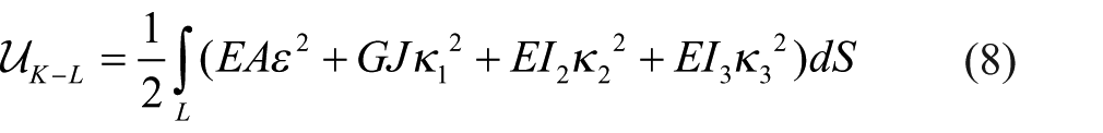
Configuration variables are positions of centreline points referred to a fixed frame,
If the rod is considered inextensible, axial forces become a consequence of equilibrium, and Kirchhoff–Love theory specializes into the 3D version of Euler–Bernoulli theory.
Other theories
Reissner
18
proposed a 3D theory in which cross-sectional rotations are independent from centreline tangents. In this theory, kinematics is based on Timoshenko’s assumption for shear-deformable beams – originally introduced for small displacements and deformations – according to which cross sections remain plane but not necessarily perpendicular to the centreline. In Reissner’s theory, as in both previously described ones, displacements and rotations may be arbitrarily large. In addition to the previous constitutive equations (7), equations relating shear forces to shear strains

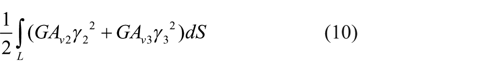
and additional terms for shear deformation energies need also be added to equation (8)
In this case, centreline positions and sectional (finite) rotations are used as configuration variables. This theory has been successfully developed by Simo 19 and other authors for the simulation of flexible beams in the context of finite elements, using finite rotations to model the behaviour of cross sections. The adjective geometrically exact has been used to refer to these models.
To put these theoretical developments into perspective, it is necessary to mention the more general Cosserat rod theory that models the rod as a space curve with three vectors attached to each point. The first is the tangent vector to the centreline curve; the other two are called directors and characterize the configuration of material fibres of the cross section. Cosserat rods were developed by Green et al. 20 on the basis of Cosserats’ 21 theory for directed continua.
Both Reissner–Simo and Kirchhoff–Love theories can be classified as special cases of Cosserat rods: in the first case, directors are chosen orthonormal in the undeformed state and are constrained to remain orthonormal during the deformation; in the second (Kirchhoff–Love), orthogonality to the tangent vector is also enforced. More complex theories considering out-of-plane deformation modes of cross sections have been developed by other authors (as Simo and Vu-Quoc 22 or Hodges 23 ) although their increased number of variables makes them more difficult to apply to shape finding of bending-active structures.
Types of discretization in DR procedures for flexible rods
Two groups of discretizations can be found in the literature: (1) finite-difference-like discretizations using 3 or 4 DoFs per node and (2) finite-element-like methods with 6 DoFs per node. The main distinction is found in the way strain measures and internal forces exerted to model nodes are evaluated.
In finite-difference discretizations, discrete strain measures at nodes are deduced from difference schemes between nodal degrees of freedom using groups of two, three or four nodes. Internal forces acting on nodes may be calculated either (1) using the discrete strain measures (assuming linear constitutive behaviour) and ad hoc equilibrium relations or (2) deriving expressions of the internal forces from energy methods and discretizing these expressions by means of finite-difference schemes.
In the case of finite-element-like discretizations, the link between nodes is considered as a beam finite element. Relations between element end forces and relative displacements/rotations of end-nodes are derived making use of beam theory and energy methods. In the following sections, we review the main contributions in each group.
Finite-difference discretizations
In this group, we are placing in chronological order the contributions by Adriaenssens and Barnes, 24 Barneset al., 25 Du Peloux et al. 26 and D’Amico et al. 9
Adriaenssens and Barnes
24
is based on the Euler–Bernoulli theory with the extensibility assumption. In a certain configuration, axial strains
and the constitutive equation (1)
Discretization in Adriaenssens and Barnes. 24
Adriaenssens and Barnes prove that, for isotropic cross sections (sections with uniform second moment of area), torsional moments are related to bending moments through an equilibrium equation and no additional forces due to torsion are needed for the DR procedure. Thus, shear forces are vector-added to link (axial) forces in order to compute residual forces acting on each node, and the DR procedure can be performed. In this way, only 3 DoFs per node are needed, and the simplest beam theory is used in the process, with the counterpart of the limitation imposed to cross sections, which need be square or circular shaped (full or hollow).
Barnes et al.
25
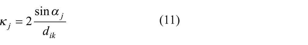
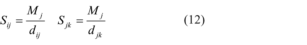
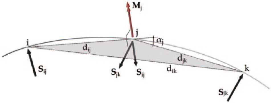
account for the case of non-uniform cross sections: in addition to considering the effect of bending through three-node in-plane shear forces as in the previous reference, out-of-plane shear forces acting on four-node groups are calculated using the constitutive equation for torsion (equation (7))
Discretization in Barnes et al. 25
where
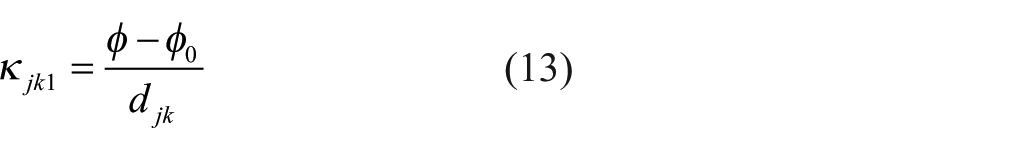
The method proposed by Du Peloux et al. 26 is close to recent developments in the field of computer animation (Bertails et al. 27 and Bergou et al. 28 ) which relate the geometry of discrete curves (an ordered set of nodes) to their mechanical behaviour using a finite-difference scheme (Figure 3). In this reference, the minimal set of degrees of freedom per node that keeps full consistency with Kirchhoff–Love theory is used: 3 DoFs for nodal positions and one rotational DoF to keep track of torsion. The latter measures the angular difference between cross-sectional material (principal) frames and torsion-free (Bishop) frames. A discrete measure of oriented curvatures using the coordinates of three consecutive nodes is employed. Torsional strains are calculated as finite differences between nodal torsional rotations.
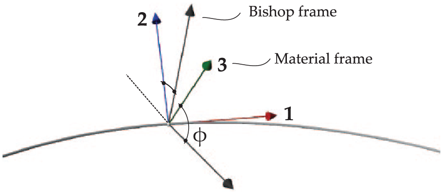
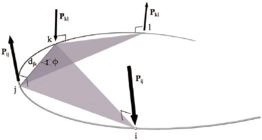
Discretization in Du Peloux et al. 26
In order to calculate nodal forces and twisting moments, Du Peloux et al. discretize the expressions of the internal forces and torsional moment in the rod, obtained as derivatives of the elastic deformation energy with respect to positions and torsional rotation. A simplifying assumption for the evaluation of the derivatives is that torsional waves propagate in an instantaneous manner compared to bending waves. The discretization of internal forces and twisting moments to obtain forces and moments acting on nodes follows a finite-difference scheme. This computation depends on the torsional stiffness
D’Amico et al. 9 make also use of a discrete approach to 3D curved rods as Du Peloux et al. It can be considered an improvement of Barnes et al. because it keeps track of the angular difference between material frames and Bishop frames in case that torsional constraints are imposed at the ends of the rod. The orientation of tangent vectors at nodes is found using Catmull–Rom interpolation; the other two vectors of the Bishop frame are found by parallel transport and then rotated to obtain the material frame. However, in contrast to Du Peloux et al., these rotation angles are not considered DoFs of the system, but initially given data. Curvatures and torsional strains are calculated operating with coordinates and frame orientations at a given node and the immediately adjacent ones (three-node groups). The total moment at a node is the result of vector-adding the components given by constitutive equation (7). Nodal shears acting on every node of a group of three are calculated imposing equilibrium with the total moment at the mid node; they are vector-added to forces from subsequent groups and to the axial link forces at nodes in a similar fashion as in Barnes et al. to calculate residuals for DR. This setup makes, therefore, use of Kirchhoff–Love theory but forces the orientation of the principal axes at a node to keep a fixed angle to the corresponding three-node plane due to the restricted number of DoFs.
Table 1 includes a summary of the main features of finite-difference-like parametrizations. Moreover, all references use equilibrium relations to obtain nodal forces for the DR process, excepting the one by Du Peloux et al. that evaluates internal forces as derivatives of the deformation energy with respect to kinematic variables.
Comparison between references using finite-difference-like discretizations.
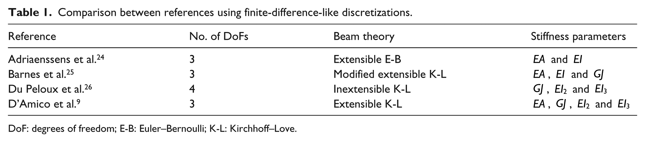
DoF: degrees of freedom; E-B: Euler–Bernoulli; K-L: Kirchhoff–Love.
Finite-element discretizations
The following references have been included in this category: Li and Knippers, 29 D’Amico et al., 30 D’Amico et al. 31 and Senatore and Piker. 32 They base on previous work by Williams thoroughly explained in Adriaenssens. 33 All of them share a common implementation feature that allows their classification into a well-established formulation for flexible rod finite elements: the co-rotational formulation. The rod is discretized into elements that can undergo large rotations, but at local level, use small-displacement/rotation relationships. We have also included Bessini et al. 34 that implements Reissner–Simo model, which is capable to deal with large rotations of cross sections with no limitation to their relative magnitude at the element level.
The proper numerical treatment of large rotations is a main concern in the computational solution of this type of problems. This fact was readily recognized by Argyris 35 to which the reader is referred for a detailed account of the following ideas. From a mathematical point of view, a rotation is an element of the special orthogonal group SO(3). The elements of this non-additive and non-commutative group can be numerically represented in several manners. Before reviewing the co-rotational formulation, the following section summarizes (in a non-exhaustive manner) the most important alternative parametrizations for rotations.
Parametrization of finite rotations
Rotations, as members of the special orthogonal group, can be represented by means of 3 × 3 orthogonal matrices
Euler’s theorem establishes the equivalence between the matrix representation of rotations and the pseudo-vectorial representation
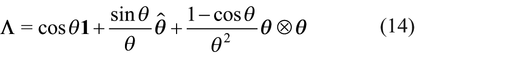
where
An alternative pseudo-vectorial three-parametrization consists in using
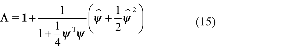
This alternative pseudo-vector has been partially used by Williams (Adriaenssens 33 ) and by D’Amico et al.30,31 (we will expand on this in the next section).
Other classical three-parameter representations, as Euler’s angles or Cardano’s angles are not advantageous compared to pseudo-vector representations and therefore haven’t found use in mechanical modelling of slender beams.
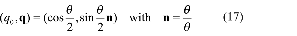
An alternative system to represent rotations is the use of unit quaternions. They are four-tuples of real numbers

Unit quaternions and rotation pseudo-vectors are related as follows
Quaternions are endowed with an algebra that provides an efficient tool to operate with rotations; this fact and the limited number of parameters compared to rotation matrices make unit quaternions a preferred choice to store and keep track of rotations.
Argyris
35
showed that the exponential operator acting on a skew-symmetric matrix,

Spins have been used as rotational DoFs for finite element implementations based on Reissner’s beam theory (Simo 19 ). They have been also used to update nodal frames in the finite-element-based discretizations that will be reviewed in the next section.
Discretizations based on the co-rotational formulation
The co-rotational technique was initially proposed in the 1970s by Wempner and by Belytschko et al. (Crisfield, 38 which includes a review of the history and the essentials of this method.)
The discretization associated with the co-rotational formulation splits the rod into two-node elements; at a given instant, the configuration is defined by nodal positions and nodal frames. The large-displacement/rotation mechanical problem is divided into two sub-problems: (1) modelling the mechanical behaviour of finite elements between nodes in terms of local displacements and rotations, and relating the latter to the changes in positions and orientations of each node; (2) keeping track of changes in nodal positions and nodal frames, with no restriction in their magnitude.
The first sub-problem requires to define and keep track of element frames, in order to quantify angular differences with nodal frames (Figure 4). If the discretization is sufficiently refined, these differences will be small, and the element behaviour can be even modelled with a linear beam theory, or considering moderately large displacements and small rotations.
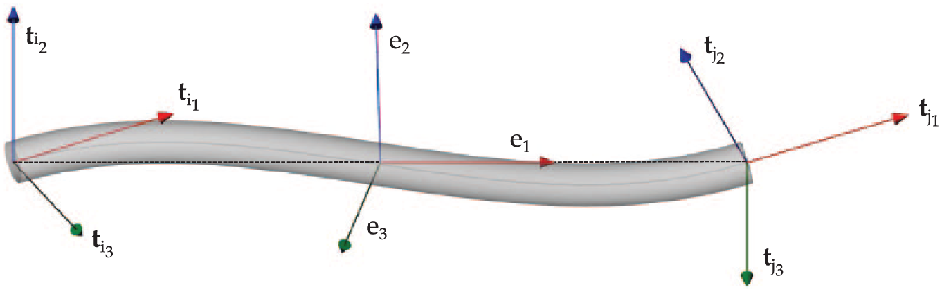
Co-rotational setup.
Nodal unit base vectors


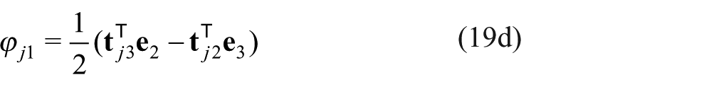
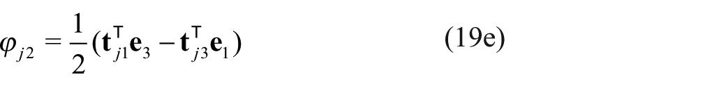
For explicit problems, once nodal rotations are known, linear beam relations between forces, moments, displacements and rotations in a beam can be used to get the applied moments and forces at the ends of each element. Alternatively, axial force–dependent non-linear terms could also be used to obtain end forces and moments. Force and moment residuals


Because there is no need to exactly reproduce the dynamics in the DR process, an isotropic inertia tensor may be chosen in order to simplify equation (20b)

With the selected time-integration technique, nodal displacements ∆
The second sub-problem involves updating large rotations of nodal and element frames from a given configuration to the next. In the case of nodal frames, the multiplicative update from equation (18) together with Rodrigues formula (14) to evaluate the exponential are used

for node
All reviewed references in this group use the co-rotational framework, with some differences in the rotation updating schemes and the mechanical model for the beam element.
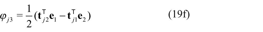
A simplification, common to all references, is to avoid the introduction of full element frames: only


Simplified co-rotational setup.
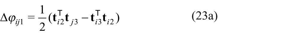
Considering that equations (19a)–(19f) were already an approximation, the simplified version requires a fine discretization in order to neglect terms that involve element frame vectors
There are some differences in the way that spins
With regard to the mechanical modelling of the beam element, Li and Knippers use linear stiffness relations corresponding to a (linear) Kirchhoff beam between nodal local displacements and rotations and local end forces.
However, Adriaenssens
33
describes the way followed by Williams to compute element end forces and moments. First, non-linear strain measures (elongation
D’Amico et al.30,31 adopt the same setup. The first reference has a summary of the resulting expressions. It is remarkable that the axial force has non-linear terms as well as rotation dependent terms due to the structure of the adopted elongation strain, and the end bending moments have geometric terms depending on the axial force, added to the standard linear terms as used by Li and Knippers.
In order to transform the scalar values into oriented force and moment terms, all references in this group need to make up for the lack of element frame vectors
and (2) calculating end shear forces such that the element is in equilibrium of moments, and vector-adding them to the oriented axial forces to get force vectors acting at element ends.
The reviewed parametrizations based on the co-rotational formulation have very similar features: all of them use 6 DoFs, rely on Kirchhoff–Love beam theory and therefore use the corresponding stiffness parameters
Discretization based on the geometrically exact model
Simo
19
and Simo and Vu-Quoc
39
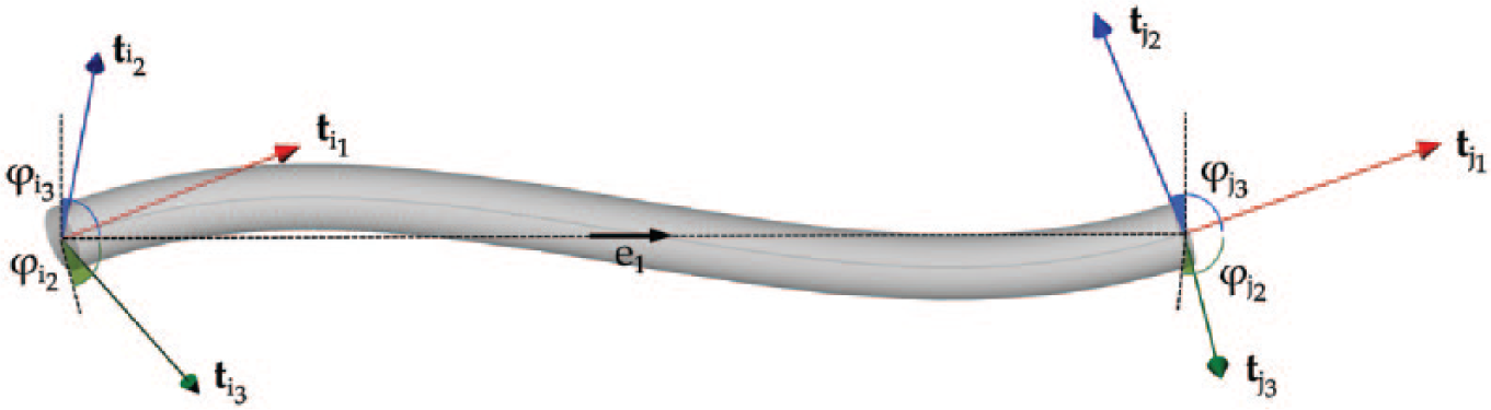
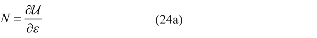
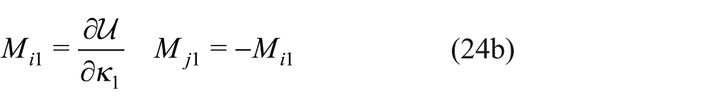
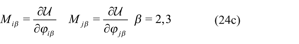
carried out the first finite element implementation of Reissner’s model. The implementation is termed geometrically exact in the literature, because of the mathematically exact treatment of rotations. The element kinematics considers that centreline positions


The first vector gathers the elongation and the shear strain components; the second one is a measure of the rate of rotation of cross sections along the centreline. Note that, in general, cross-sectional normals won’t be coincident with centreline tangents due to shear deformation. Linear elastic constitutive relations are implemented in a straightforward manner considering six stiffness parameters:
The simplest implementation discretizes the structure into two-node elements, selects displacements ∆
Discussion
The main argument for developing 3-DoF finite-difference-like discretizations for form finding of bending-active structures is that coupling of rotational DoFs with translational DoFs and axial stiffness is the cause of ill-conditioning of the DR process. 25 Adriaenssens 33 compared the results of the 3-DoF model with those obtained using the 6-DoF discretization proposed by Williams for the simulation of the planar elastica problem with different load magnitudes and found that while both methods provided similar accuracy in the geometry of the solution, the 3-DoF model was remarkably faster. This was an expected conclusion because the latter model is substantially simpler. It is interesting to follow how the 3-DoF model has been gradually refined, from the one first developed by Adriaenssens,24,33 only valid for isotropic cross sections, through the model by Barnes et al. 25 that considers non-isotropic cross sections but models out-of-plane bending stiffness through the introduction of an artificial torsion constant affecting the torsional stiffness, to the model by D’Amico et al. 9 that calculates Bishop frames to refer the orientation of the bending axes and therefore uses all strain measures and stiffness constants of the Kirchhoff–Love beam at a higher computational cost than the other two models. The fact is that using only translational DoFs imposes an internal constraint to the orientation of the section axes: in the model by Barnes, the reference bending axis at a node is forced to stay in the plane formed by the node and the two adjacent ones; in the model by D’Amico, it is forced to keep a pre-determined orientation with respect to the Bishop frame defined by the discrete curve in each step.
The 4-DoF discretization by Du Peloux et al. offers a trade-off between computational cost and model accuracy, as it uses the minimal set of parameters that is fully consistent with Kirchhoff–Love theory. Although the theoretical foundation presented by the authors considers the inextensible Kirchhoff model, the computational implementation imposes the inextensibility constraint through node-to-node directed penalty forces that can be adjusted to be actual axial forces by using the real cross-sectional axial stiffness.
All 6-DoF finite-element-like discretizations share the disadvantage of requiring the highest number of parameters. The comparative computational cost with respect to 4-DoF discretizations remains to be analysed, because in the latter, the cost of keeping track of Bishop frames and material frames during the process might be comparable to the cost of updating nodal frames in the former. In spite of the conditioning problems of 6-DoF discretizations mentioned by Adriaenssens and Barnes, all reviewed references report an adequate performance of their models. A further advantage of these discretizations is the ability to directly integrate the result of form finding into a finite element tool to further analyse the structural behaviour under additional loads, or to trace the construction sequence back to an undeformed configuration. Integration with an analysis tool may be much more difficult in the case of finite-difference discretizations (with perhaps the exception of the 4-DoF implementation). A particular feature of the implementation by Bessini et al. is the ability to deal with shear-deformable structures. In the realm of active bending, this can be applied to the design of structures with members consisting of two or more layers of laths when considered as structural elements with large shear deformations, such as the Mannheim Multihalle.
Final remarks
Computational form finding of bending-active structures is a challenging problem. DR has been used in many references as the basis for form finding; however, under this common umbrella, approaches show significant differences in both the underlying beam theory and the type of discretization.
Discretizations have been classified into two groups: finite-difference-like and finite-element-like. Both rely on a distribution of nodes along the centreline of a flexible beam and consider masses (and inertias) to be lumped at nodes. The first group evaluates strains and internal forces acting at nodes using the relative positions of groups of nodes and the stiffness parameters of cross sections, whereas the second group treats the links between elements as finite elements and evaluates strains and internal forces from the configuration of adjacent nodes.
Finite-difference discretizations use 3 or 4 DoFs per node, and range from simple implementations based on planar Euler–Bernoulli theory, suited for isotropic cross sections, to more complex models based on 3D Kirchhoff–Love theory that account for torsion and spatial bending in an accurate way. References report advantages in terms of computational cost and robustness of the DR algorithm.
Finite-element discretizations employ 6 DoFs per node and are built on Kirchhoff–Love or Reissner–Simo beam theory. Reviewed references implement simplified versions of co-rotational elements or geometrically exact elements. Their main advantage is that results from the form finding process can be directly exported to finite element models.
The reviewed references show that there is a range of available models/discretizations to be applied in DR algorithms for very flexible beams. However, there are still unexplored questions that are worth studying, as carrying out performance comparisons between models, or even implementing alternative discretizations for flexible beams that have been tested in the finite element realm.
Footnotes
Declaration of conflicting interests
The author(s) declared no potential conflicts of interest with respect to the research, authorship and/or publication of this article.
Funding
The author(s) disclosed receipt of the following financial support for the research, authorship, and/or publication of this article: The financial support from the Spanish Ministry of Economy and Competitiveness through grant BIA2015-69330-P (MINECO) is gratefully acknowledged.