






Abstract
There are pronounced differences in the productivity of local economies in England and Wales, with some areas thriving whilst others struggle with a legacy of de-industrialisation. This article relates productivity differentials to industry and occupation structure. Doing this facilitates the extrapolation of a metric for ‘productive employment base’ at local authority level. Using this measure, progress is examined for local authority areas in England and Wales during the period 1998–2012. Maps are produced of local areas making greatest gains. These are termed ‘emerging productive economies’.
Keywords
Introduction
A recurring theme of local policy making is the divergent success of the UK’s local economies and labour markets. Debates on overlapping themes of regional divergence, local competitiveness and skills reinforce the message that some places are doing rather better than others according to most measures of economic success. Centre for Cities (2012) reviewed the progress of 64 largest towns and cities against the context of the ongoing economic downturn, revealing an all too familiar picture of disparities between high thriving places (read Cambridge; highlighted in the report) and struggling local economies (read Hull; similarly highlighted).
These differences come as no great surprise given a backdrop of evidence on differences in local competitiveness (Huggins and Thompson, 2010); pronounced local unemployment differentials (House of Commons, 2012); and differences in local employment skills (Green and Owen, 2006). The north-south divide, long established and evidenced (see Blackaby and Manning, 1990) is very much persistent today with the flourishing geographies of opportunity (see Webber and Swinney, 2010) largely based in and around the capital.
What emerges from the literature on local competitiveness is the notion that some places have the right kind of jobs – in terms of industry structure and occupational composition. Analysis presented in HM Treasury (2001, 2003) demonstrated that differences in local productivities can be accounted for in terms of industry and occupation composition using a fairly rudimentary statistical model. Having high concentrations of high productivity (high value added) sectors of employment backed by a strong knowledge base in key professional areas, in turn facilitated by world-class skills (Leitch, 2006) is the formula for the high road to economic prosperity. These ideas are linked to a burgeoning research around key high sectors of the economy, and in particular so called Knowledge Intensive Business Services or KIBS (see DTI, 2007; Muller and Doloreux, 2009; UKCES 2012), and also more generally in relation to the so called ‘knowledge economy’ (for example see Hepworth et al., 2005; Levy et al., 2011).
The notion that local economies should strive to get the right mix of jobs (i.e. ones which are productive in a monetary sense) is also related to the emerging literature around ‘quality of jobs’ (see Goos and Manning, 2007; Jones, 2009; Jones and Green, 2009). This literature acknowledges that in a market economy each job has a marginal productivity value associated with typical earnings for that job category, where jobs are defined by detailed occupation category/industry sector. The papers referred to conceptualise and develop a framework for measuring changes in the profile of job quality. Applying this at local level to maximise productivity, or at least to increase productivity over time, the focus should therefore be on increasing quantities of some jobs and not others.
The purpose of this article is twofold: firstly to pin down precisely which industries and occupations are key to driving higher productivity at local level. Undertaking this as a statistical exercise will reveal which industry/occupation mix is ‘desirable’; or most productive. This is done using standard regression methodology, utilising Gross Value Added (GVA) data available at NUTS level 3 along with data on industrial and occupational composition of employment. The next section ‘Productivity and industrial and occupational structure’ describes the methodology in detail and presents results on what constitutes a ‘productive employment base’, using the terminology adopted in the article.
The second aim is to present a dynamic picture of the changing local economic geography of England and Wales in terms of which local economies have managed to succeed in growing the right parts of their economies. This uses the ‘productive employment base’ measure developed earlier in the article. As acknowledged at the start of this article, the static picture of productivity differentials is well established and understood. However, a key question is whether struggling local and regional economies, with an inheritance of de-industrialisation, are showing signs of turning their situation around by creating productive employment. In doing this we are able to drill down below NUTS units to present a detailed picture of changes over time, since 1998, in 348 local authority areas in England and Wales. Maps are produced of what are termed ‘emerging productive economies’ – those local authority areas where the balance between the most and least productive jobs has shifted most positively over time. The third section of this article discusses the data and methodological approach and presents findings while the fourth draws conclusions.
Productivity and industrial and occupational structure
Productivity data
Productivity is measured using estimates of GVA per head of population. These are provided via open public access by the Office for National Statistics (ONS). The GVA data used in this study utilises the December 2011 release (providing 2010 GVA estimates), the latest available estimates at time of writing. The GVA estimates are available by local spatial unit and by industry, as described below.
The lowest denomination of productivity data at local level in England and Wales is available for Nomenclature of Units for Territorial Statistics (NUTS) level 3 regions. NUTS is a hierarchical classification of local units available for the European Union. For England and Wales, the third level of the hierarchical classification (NUTS3) corresponds approximately to unitary authority area, counties, or sub-regions (typically former metropolitan areas, or groupings thereof). For England and Wales (i.e. in the dataset utilised for this study) there are 105 NUTS3 spatial units; based on the NUTS 2003 classification.
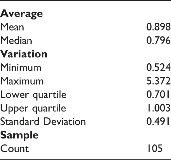
The unit of comparison for modelling local area variation is the local productivity ratio, which is defined for the purposes of this study as the ratio of local GVA per head (for NUTS unit i) to GVA per head figure for England and Wales as a whole. The data in Table 1 summarises the descriptive statistics of local productivity ratios across 105 NUTS3 units in England and Wales and Figure 1 provides a picture of the shape of the distribution. The bulk of the distribution of productivity ratios is below 1 (parity with the England and Wales average) reflecting the skewed shape of the distribution with a small number of local units, predominantly in London and the South East of England, having higher than average productivity. At the extreme, the Inner London (West) sub-region has a productivity ratio of 5.3 times that of England and Wales, reflecting the anomalous nature of this area which contains the City of London financial centre but is sparse in population.
Local productivity ratios England and Wales: Frequency distribution. Local productivity ratios England and Wales: Summary statistics.
Linking productivity to industrial structure
This section links local productivity differentials to local industrial structure. To this end, the GVA data provided by the ONS provides a breakdown of GVA by industry by NUTS3 local area. The industrial breakdown is provided for 10 industry groupings based on the Standard Industrial Classification (SIC2007) classification, based on place of work (rather than place of residence). This data provides a proxy for local industry composition array based on the percentage contribution of each industry to total GVA.
Utilising this data, a weighted regression is run with dependent variable defined as the natural logarithm of the local productivity differential for unit i. The logarithm specification is preferred, given the skewed nature of the underlying distribution (as shown in Figure 1). The explanatory variables consist of the full array of percentage GVA contributions from the 10 industries. The regression is run without a constant in order to avoid the dummy variable trap. Finally, the regression is formulated using weighted least squares, where case weights are based on total local GVA, so that larger local economies (e.g. big city sub-regions) are given more weight in the regression model.
Regression model of local GVA against local industrial composition.

Note: *Indicates statistical significance at the 5% error level; ** indicates statistical significance at the 1% error level.
Whilst the coefficients of the linear regression model indicate different weightings for industrial sectors as a predictor of local GVA, it is useful to develop a more pragmatic measure based on a simple addition of industry concentrations. To this end, the following measure of industrial mix is proposed (see below). For the purpose of this article this is termed the Productive Industry Balance.
Although crude in econometric terms, this ‘rule of thumb’ metric can be more intuitively applied to data on local employment, as developed in the next section of the article. It should also be noted that dropping the linear weights and using this simpler alternative results in only a small loss in predictive power. Regressing the logarithm of the local productivity differential against the crude Productive Industry Balance measure (see bottom panel Table 2) achieves an excellent fit, with adjusted R-squared of 87.5%. This compares to 89.5% for the final regression model.
Linking productivity to occupational structure
This section links local productivity differentials to local occupation (as opposed to industry) structure. To do this, additional data is required regarding occupational structure at NUTS3 level. This is available from the Annual Population Survey (APS), contemporaneously at 2010, but using resident-based rather than workplace-based employment data (workplace employment counts were not available for this time period). This data is utilised to construct an array of occupational composition of percentage of employment by 25 detailed occupation categories, based on the Standard Occupation Classification (SOC). SOC2000 sub-major group categories are used due to readiness of comparison to previous periods, as will become clear in the next section.
Utilising this data, a weighted least squares regression is run as previously with dependent variable defined as the natural logarithm of the local productivity differential for unit i, and total GVA as weights. The explanatory variables now consist of a full array of percentage employment for each of the 25 occupation categories.
A key issue to consider here is that the dependent variable measures GVA differential by local area according to location of place of work whereas occupation structure reflects place of residence. As the vast majority of people live and work in the same sub-region this need not necessarily pose a problem. However, where commuting flows are large, statistical comparisons may be misleading as favourable occupational structures may not reflect favourable local industrial conditions, or vice versa. This will be particularly the case in London and the South East where commuter flows are large from the periphery to the centre. Thus, a pragmatic modelling decision is made, as follows. The regressions are run at NUTS3 level, as described above, but excluding NUTS3 units in London (5 areas in total) and immediate surrounding areas which are spatially adjunct to the boundary of Greater London and thus proxying reasonably for a commuter belt. These NUTS3 areas are: Berkshire, Buckinghamshire, Essex, Hertfordshire, Kent, Surrey and Thurrock.
Regression model of local GVA against local occupational composition.

Note: *Indicates statistical significance at the 5% error level; ** indicates statistical significance at the 1% error level.
As with industry, the linear regression model is reduced into simple additive form, effectively imposing a simpler linear structure for application in a ‘rule of thumb’ fashion, as proposed previously. The resulting indicator of occupational structure is termed the Productive Occupation Balance, as shown below.
Regressing the logarithm of the local productivity differential against the Productive Occupation Balance (see panel 3 of Table 3) results again in only minor loss of fidelity with adjusted R-squared falling from 57.8% in the weighted model to a healthy 52.3% using the cruder indicator. It is noted, finally, comparing figures for explanatory power in Tables 2 and 3 that industry rather than occupation composition is a stronger predictor of local GVA, although it is possible that in part this reflects the imperfect mapping of resident and workplace employment.
Emerging productive economies: Local economies in England and Wales
Having established predictors of GVA productivity in terms of industry and occupation composition, this section examines changes in employment composition at local level using these indicators. The purpose of this exercise is to illustrate which local authority districts/unitary authorities (LAD/UAs) have progressed most over recent years in terms of establishing a productive economic base. Note that this second stage uses a more detailed geography than that available based on NUTS3.
Data on local employment composition
The data exercise is one of back-casting the crude industry and occupation predictors to achieve comparisons over time. This can be done using local area employment data for England and Wales which is readily available from the ONS via the NOMIS webpage. Industry comparisons are available using the workplace-based Annual Business Register (ABR) and Annual Business Inquiry (ABI). Occupation comparisons are available using Annual Population Survey (APS) data, available based on both workplace and resident counts for local authority areas. This creates a detailed geographical picture based on 348 LAD/UAs in England and Wales. Details of data construction, including dates which vary by data source, are discussed separately for industry and occupation below.
Industry by key sector using SIC2007 and SIC2003 mappings.

Workplace employment data are available from the ABI between 1998 and 2007, using SIC2003 classifications. Utilising this data, and combining with the more recent ABR data, comparisons of industrial composition at local (LAD/UA) level are constructed for the period 1998–2010.
Comparisons of occupation are more straightforward using SOC2000 sub-major group categories. Comparisons of workplace employment data are available at local (LAD/UA) level from the workplace APS between 2004 and 2012. Resident-based data can be tracked back further, with comparisons available using the 2001 census and 2012 resident-based APS data. Each of the sources uses consistent SOC2000 sub-major group occupations.
Emerging productive economies by industry
The data described facilitates comparisons of industrial composition between 1998 and 2010. The crude indicator of Productive Industry Balance is calculated for each of the 348 local areas (LAD/UAs) in England and Wales for 1998 and 2010 using the simple additive formulas shown in section ‘Linking productivity to industrial structure’ above. The derived measure gives a percentage of employment figures for 1998 and 2010, respectively, which are normalised in turn by subtracting the figure for England and Wales in the respective period (therefore in effect giving a percentage comparison relative to a zero average). The change over time is calculated for each LAD/UA. Note that measures therefore capture the change in employment composition and not change in overall levels of employment, which are not considered.
The results are presented in two ways. Firstly, Figure 2 shows the results for the whole cross section of LAD/UAs. The change in the Productive Industry Balance is compared to the original 1998 figure. Each scatter point represents an individual LAD/UA which is weighted by total employment (thereby creating larger circles for more populated local areas). The figures reveal a great deal of variation over the intervening 12-year period. What is interesting, however, is the fact that the economies achieving greatest positive transformation towards a productive industry base (i.e. those with positive values on the vertical axis) tended to be those with the highest level of initial disadvantage. This effect is shown by a negative sloping line of best fit on the chart, which is statistically significant. The larger LAD/UAs can be seen, generally although not exclusively, towards the top right of this plot.
Productive Industrial Balance by LAD/UA, 1998–2010.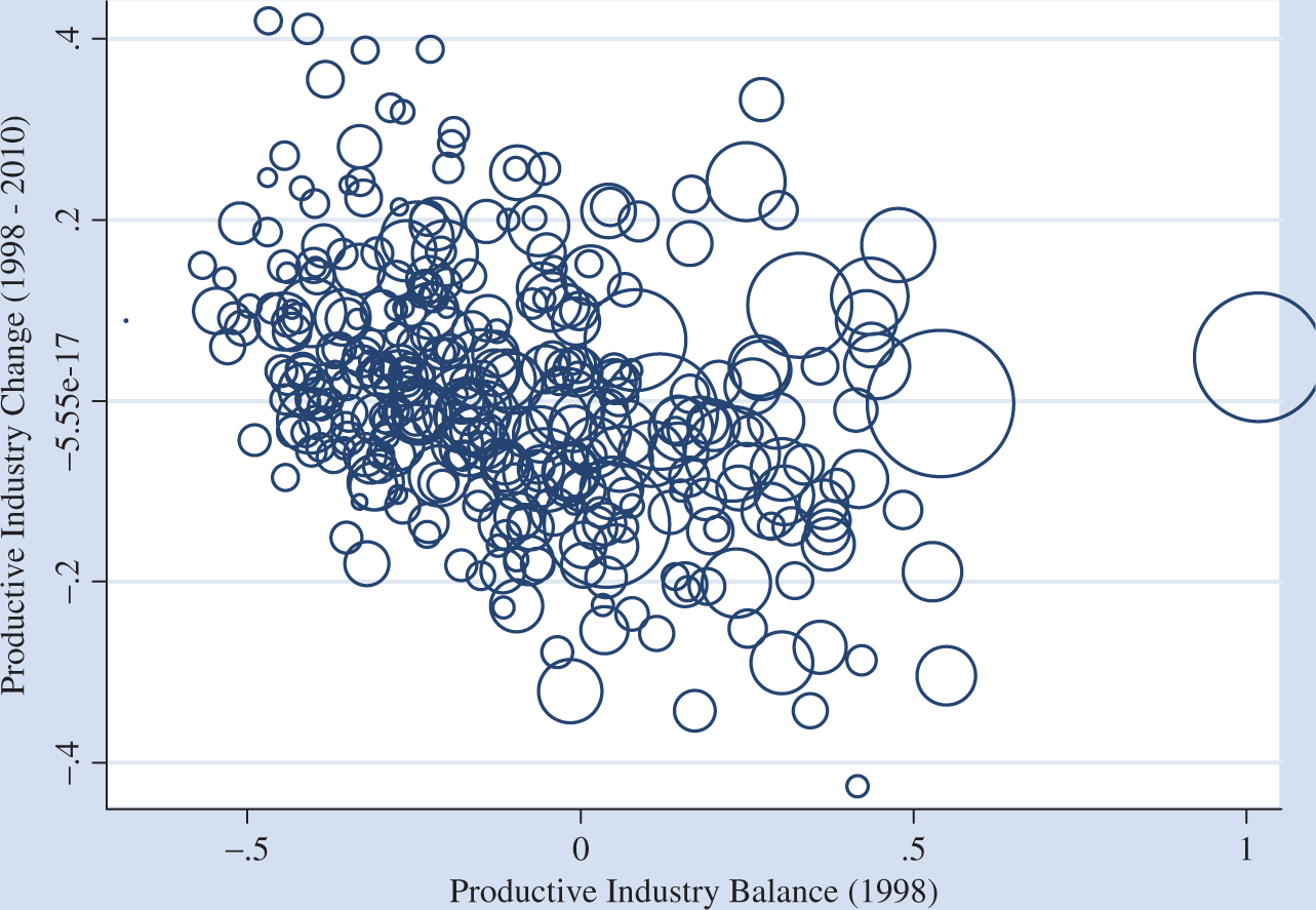
Secondly, Figure 3 maps the best performing local economies in terms of positive industrial restructuring. The normalised figures for change in productive industry balance were ranked from lowest to highest. The map shows those LAD/UAs in the upper quartile and upper decile of this distribution. For the purposes of this article, LAD/UAs in either of these categories are termed ‘emerging productive economies’. Upper decile and upper quartile categories are shown separately on the map. The map shows a dispersed pattern of emerging productive economies across all regions of England and Wales. Clear north versus south differences are not discernible. Neither pattern of development is London or South East centric. Emerging productive economies are found throughout the country, with many large rural authorities highlighted as making most progress. Whilst this appears to indicate something of a counter-urban trend, correlation of changes in productive industry balance with local authority population density was not found to be significant.
Emerging productive economies by industry of employment, 1998–2010.
Emerging productive economies by occupation
A similar set of calculations can be performed for occupation. The figure for Productive Occupation Balance is calculated for each of the 348 local areas (LAD/UAs) in England and Wales. This is done using workplace data for 2004 and 2012 and residence-based data for 2001 and 2012. The figures are normalised by subtracting the figure for England and Wales in each of the respective periods, as previously. The figures are then differenced over time, by workplace 2004–2012 and by residence 2001–2012, respectively. Note again that the differenced measures capture the change in employment composition and not change in numbers employed.
The results of this exercise are again shown in cross section of all LAD/UAs by means of a scatter plot where, as previously, scatter points represent the size of the LAD/UA in terms of total employment. Change in workplace occupational structure (2004–2012) is shown in Figure 4, whereas change in residence-based occupation (2001–2012) is shown in Figure 5. In each of these cases the correlation between initial value and change over time was not statistically significant. No statistically significant effect is detected by LAD/UA size over time. However, large city economies tend to start from a more advantaged base in terms of higher initial productive occupation balance, with large scatter circles generally found towards the right of the scatter plots.
Productive Occupation Balance by LAD/UA workplace, 2004–2012. Productive Occupation Balance by LAD/UA residence, 2001–2012.

The Productive Occupation Balance data is also mapped in Figure 6 (which shows changing occupational composition by workplace) and Figure 7 (which shows changing occupational composition by place of residence). In constructing these maps the same approach is taken as previously. The maps highlight the best performing local economies, based on positive occupational restructuring. The maps show LAD/UAs in the upper quartile and upper decile of the ranked distribution of occupation restructuring scores, with calculations done separately for workplace location and place of residence. Upper quartile and upper deciles are shown separately and local authorities in these categories are termed ‘emerging productive economies’ for the purpose of this article.
Emerging productive economies by workplace occupation, 2004–2012. Emerging productive economies by resident occupation, 2001–2012.

The maps of occupational change show some similarities by place of work and place of residence, although these are by no means identical. The distribution across regions shows a slight bias towards the South East of England, particularly based on resident occupation, with areas in and around London particularly benefiting from positive changes in employment composition. This said, progress is not limited to the South East and there are pockets of emerging productive economies in the North, and in particular the North West region (Figure 6), the Midlands (Figures 6 and 7) and South West (Figures 6 and 7).
The emerging productive economies by occupation correspond with those by industry but the association is fairly weak (correlation of 0.212 based on changes in productive industry and productive occupation balance, utilising workplace data). A small number of local authorities are identified as emerging productive economies based on changes in productive industry scores and changes in productive occupation scores by workplace and by residence, thus appearing on all three maps at upper quartile or upper decile level. These local authorities are:
Fylde; Wyre (North West); Bolsover; Blaby; Hinckley and Bosworth (East Midlands); Staffordshire Moorlands; North Warwickshire; Malvern Hills (West Midlands); Fenland; Kings Lynn and West Norfolk (East of England); Weymouth and Portland; Mendip (South West); Adur (South East).
With respect to this list, it is particularly noteworthy that these are predominantly rural areas and whilst some are formerly industrial (notably Bolsover) these areas are outside the cities and large urban conurbation. Again, this points to a counter urban trend with rural and semi-rural areas moving towards a progressive industrial and occupation structure and, by inference, diversifying away from agricultural and industrial heritage. The progressive changes in occupation by place of residence also indicate a willingness of higher skilled workers to live in these areas. Whilst the list is informative, the correlation of changes in productive occupation balance with population density was not found to be significant for either place of work or place of residence.
Conclusion
The differences in local area productivity in England and Wales are well documented and well understood. The pronounced differences in local productivity mirror spatial differences in industry and occupational structure, in turn corresponding to differences in qualifications and skills. In simple terms, London and the South East tend to have favourable industry/occupational structures with correspondingly higher levels of skills. In contrast, de-industrialised parts of the North, the Midlands and Wales fair badly by comparison. However, this is a static picture based on long-standing differences, lack of convergence and asymmetric historical processes, particularly with respect to the effects of de-industrialisation.
The results presented in this article focus on the dynamic picture. The (static) differences in GVA productivity by local area are systematically related to industry and occupation structure. By doing this we are able to identify which industry and occupation categories are the most important in generating higher productivity. In turn we can then examine to what extent the industry and occupation structure has changed progressively, i.e. in favour of industries and occupations with higher value added outputs. This methodology is applied at local authority level for England and Wales between 1998 and 2012. Local authorities making greatest gains are termed ‘emerging productive economies’, based on their position in the upper quartile of the ranked distributions of changes by industry and occupation (work-based and resident-based location); treated separately.
The results show an interesting emerging picture for local authority areas in England and Wales. In short, the maps of emerging productive economies do not correspond to stereotyped expectations of London and the South East versus the rest. The picture is more mixed than that. There is strong evidence to suggest a picture of changes in industrial structure favouring the provincial regions outside London, including the Midlands and the North. Moreover, the evidence presented in the article suggests a process of convergence by which previously disadvantaged local areas (with lowest productivity) have made the greatest gains in terms of expanding productive sectors. This bodes well for the future of these areas and happily contradicts the usual notions of two-speed economies.
The evidence on occupational restructuring is more mixed. Something of a South-East bias is observed in terms of identifying local authority areas which have made most progress in expanding the most productive occupations. However, this oversimplifies the picture. There is still a disparate regional picture with emerging productive economies in all parts of the country, according to the occupation measures. What is also interesting is that many large rural local authorities have managed to make great leaps forward not in only in terms of industry and occupation changes by place of work, but also by occupational structure of residents, in part indicating perhaps higher skilled workers preferring to live in these areas.
The geographical picture presented in this article is interesting as it is emerging. It thereby helps provide a challenge to standard economic geographies of productivity in England and Wales.
