Using InVivoStat to perform the statistical analysis of experiments

Abstract

The need to improve reproducibility and reliability of animal experiments has led some journals to increase the stringency of the criteria that must be satisfied before manuscripts can be considered suitable for publication. In this article we give advice on experimental design, including minimum group sizes, calculating statistical power and avoiding pseudo-replication, which can improve reproducibility. We also give advice on normalisation, transformations, the gateway analysis of variance strategy and the use of p-values and confidence intervals. Applying all these statistical procedures correctly will strengthen the validity of the conclusions. We discuss how InVivoStat, a free-to-use statistical software package, which was designed for life scientists, especially animal researchers, can be used to help with these principles.

Keywords

Confidence interval gateway ANOVA InVivoStat nested design pseudo-replication statistical power transformation

Introduction

There has been much discussion in the literature regarding the poor reliability and reproducibility of the results of animal experiments (e.g. Gore and Stanley, 2015; Kilkenny et al., 2009; Nature Editorial, 2014; Peers et al., 2014; U.S. National Institutes of Health, 2014). Common problems include: the lack of randomisation and blinding of experiments (Macleod et al., 2009, 2015), leading to biased results; choice of sample size (Button et al., 2013), leading to under-powered statistical tests; and inappropriate experimental design and statistical analysis (Kilkenny et al., 2009), leading to potentially more animals being used than is necessary. As well as the above issues, Bate and Clark (2014) describe many of the potential pitfalls that should be avoided when conducting animal research, including: the use of poor experimental designs that do not account for nuisance sources of variability; incorrect, or no, randomisation of study material; and performing sub-optimal statistical analyses that fail to make use of all available information.

These concerns have been addressed by several initiatives. For example, the ARRIVE guidelines provide a framework for reporting and conducting animal research (Baker et al., 2014; Kilkenny et al., 2010; McGrath and Lilley, 2015). The NC3Rs has also developed the Experimental Design Assistant (EDA), https://eda.nc3rs.org.uk, which is a web-based resource that facilitates and validates the design of experiments and statistical analysis of the data. This package enables researchers to generate a schematic figure that describes their experiment, which is then interrogated to identify issues that could undermine the validity of the conclusions.

However, reproducibility of research findings also depends on the combination of a valid experimental design and valid statistical techniques. To support that need, a free-to-use statistical software package, InVivoStat (www.invivostat.co.uk), has been designed specifically to help researchers analyse the data generated from their experiments (Clark et al., 2012). InVivoStat is an implementation of the R language, and hence inherits the power of R. While advanced users may prefer to use R directly, the benefits of using InVivoStat are the inclusion of dataset checking facilities, improved output that contains tips and advice for users and the selection of R parameter settings that have been independently verified. The package, which can also be used in combination with the EDA, implements many important statistical analyses, such as analysis of variance (ANOVA) and more advanced techniques (e.g. repeated measures mixed models).

In this article, we discuss some common problems and controversies concerning the application of statistics in animal experiments and go on to explain how InVivoStat can help to avoid them. This is important because ensuring compatibility of the experimental design and statistical analysis, before starting the experiment, can reduce considerably the number of animals needed to reach a valid conclusion. We further consider the ways in which InVivoStat offers alternative approaches and explain why they may be preferable in certain situations. Complete ‘walkthroughs’ and information regarding the examples presented in this paper, including copies of the datasets, are included in the Supplementary Material online.

Implementing guidelines regarding experimental design

On minimum group sizes

It is often proscribed that statistical analysis should not be performed if the number of experimental units within each group is less than five. In our view, such advice applies primarily when the statistical analysis involves comparing pairs of group means, such as when using t-tests or post-hoc tests. There are other types of statistical analyses where smaller group sizes are not only adequate but also (from a 3Rs perspective) more appropriate. One example is experiments conducted to estimate the dose–response relationship, where this is modelled by fitting a four-parameter logistic curve (Liao and Liu, 2009). Such analyses can be performed using InVivoStat’s Dose–Response Analysis module. For a fixed total number of animals, increasing the number of dose concentrations in the design, with fewer animals on each individual dose, can result in more reliable estimates of the parameters that define the logistic curve. In such analyses, n=3 animals per dose may be sufficient. Bate and Clark (2014) describe a simulated example where reducing the number of animals from seven to three per dose had negligible impact on the overall conclusions of the statistical analysis; see also the experiment described in Example 1.

Example 1: dose–response assessment

An experiment was performed to evaluate the effect of the novel 5-HT₆ agonist WAY-181187 on ventral tegmental area dopaminergic neurons (Borsini et al., 2015). The effect of cumulative doses of WAY-188187 (50, 100, 200, 400, 800 and 1600 µg/kg given intravenously) were recorded after stereotaxic implantation of recording electrodes into the ventral tegmental area of anaesthetised rats. The response was expressed as a percentage change in the basal firing-rate, which was based on comparisons of the response to drug with a control group. This approach needed sample sizes of n=5 in the treated group and n=4 in the control group. The results are presented in Figure 6 of the original paper. If the researchers had decided instead to model the WAY-181187 dose–response relationship, using a logistic curve, rather than fit a categorical ‘Dose’ factor to compare individual doses back to control, then only three animals per group could have been sufficient (Figure 1).

Figure 1.

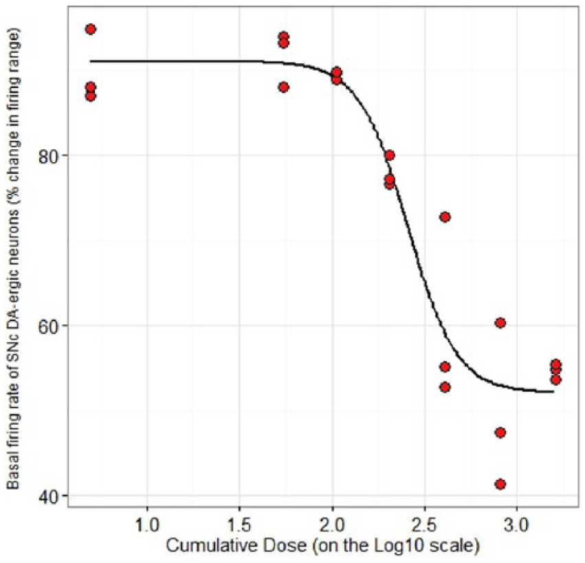
Non-linear model prediction and individual data for Example 1.

From this analysis, we can estimate the underlying dose–response relationship and identify the dose that will reduce the firing rate by 50% (the ED50), which is estimated to be approximately 250 µg/kg. Assuming the effect observed at a dose of 200 µg/kg was biologically relevant, a power analysis revealed that, when using a t-test to compare the 200 µg/kg group mean with the control mean, six animals per group would be required to achieve a statistical power of 90%.

When all treatments are administered to all animals, and hence the differences between the treatments are assessed within-animal, then n=4 can be sufficient. Examples include safety assessments or telemetry studies, which are based on dose-escalation, or cross-over designs (Aylott et al., 2011). Such analyses can be performed within InVivoStat using the Paired t-test/within-subject Analysis and Single Measures Parametric Analysis modules, respectively.

Example 2: split-plot-type trial and dose-escalation trial

Shoaib et al. (2003) performed an experiment to assess the effect of bupropion (1, 3 or 10 mg/kg) or saline 30 min before injection of nicotine (0.025, 0.05, 0.1 or 0.2 mg/kg, given subcutaneously) on rats trained to discriminate nicotine from saline. The experiment was conducted using a two-lever discrimination chamber under a schedule of food reinforcement.

In the original experiment, the sequence of treatment allocation for each rat was randomised. In this case an ANOVA approach can be used to analyse the data: the factor ‘Animal’ can be included as a blocking factor. This approach accounts for animal-to-animal variability and the effects of different doses are compared with the within-animal variability. Such an analysis can be performed using the Single Measures Parametric Analysis module within InVivoStat (see Section 4.1 in the Supplementary Material).

If the researchers had decided to administer the treatments to the animals in the same dose-related sequence/order, then the experiment would have been a dose-escalation trial. Because the order of administration is non-random, then the levels of the ‘Dose’ factor are not randomised. Moreover, the drug effects in each animal will be related (over time) and so a repeated measures analysis should be used. Such analyses can be performed within InVivoStat using the Paired t-test/within-subject Analysis module (see Section 4.2 in the Supplementary Material).

When performing a more conventional statistical analysis, to require a minimum sample size of n=5 is sensible. It implies that the individual group means are more likely to be reliable estimates of the true effects than if smaller group sizes had been used. However, it is also necessary to consider the accuracy of the estimate of the underlying variability, as indicated by the size of the residual degrees of freedom. Differences between the group means are assessed against this estimate of the variability, which also needs to be reliable as a consequence. So, even if the group means are reliable, statistical comparisons between them may not be reproducible if the estimate of the variability is not also reliable.

InVivoStat does not apply a lower limit on group size, but it does consider the size of the residual degrees of freedom: if the degrees of freedom is less than 5, then a warning is given. For an experiment involving two groups, this equates to n=4 being ‘acceptable’. If a covariate and a blocking factor at two levels is also included in the statistical model, then n=5 is the minimum sample size per group that will avoid the warning message.

If the treatment factor has more than two levels, or if there are more than two treatment factors, then the InVivoStat warning is unlikely to trigger for sample sizes of three or more. Note that if there are two factors in the experimental design, then the researcher may be able to compare the overall group means of each of the two factors, rather than compare the levels of the two-factor interaction, and hence benefit from the ‘hidden replication’ within the design (Selwyn, 1996). For example, if a design involves two factors (Sex and Treatment) each at two levels, with n=4 animals at each combination of the factors, then there would be n=8 animals for a comparison of the overall effect of the treatments. However, this comparison would ignore the Sex factor, and so can only be carried out if there is no significant interaction between Treatment and Sex (i.e. the effect of the treatments is the same for males and females). The converse applies when testing for overall sex differences.

On statistical power analysis

Statistical power indicates the likelihood of achieving a statistically significant test result in an experiment, assuming that the biological response is real. It is increasingly common to see a requirement that researchers conduct an a priori power analysis to estimate a suitable sample size. Factors that influence sample size include: the variability of the responses; the desired statistical power; and the magnitude of the biologically relevant effect (Festing et al., 2002). However, increasing the size of the sample increases the likelihood that small effects will turn out to be statistically significant and so a clear definition of the threshold for statistical significance is also needed. As has been acknowledged by others, it is not acceptable to increase sample sizes merely to attain statistical significance. In this context, it is useful to investigate how altering the size of the effect of interest influences the statistical power and sample size.

InVivoStat (Power Analysis module) provides a graphical tool to investigate the suitability of the choice of sample size. The user enters an estimate of the variability and a range of biologically relevant effects and then InVivoStat produces a series of power curves for each effect size. This approach allows the user to visualise the impact of varying both the sample size and the biologically relevant effect on the statistical power of the proposed experiment (Example 3).

Example 3: power analysis assessment

A researcher needs to identify a suitable sample size for their next experiment. A pilot study produced an estimate of the variability of the data (variance = 4). What constitutes a biologically relevant effect in the animal model is not certain and so it is decided to investigate a range of plausible changes relative to the control (between 1 and 4). A true effect of less than 1 would be too small to be of any interest, whereas it is unlikely that an effect greater than 4 could be achieved in practice. The researcher also decides that the experiment should be performed only if the statistical power is greater than 70%.

The power curves generated by InVivoStat’s Power Analysis module in this example are given in Figure 2 (see also Section 5 in the Supplementary Material).

Figure 2.

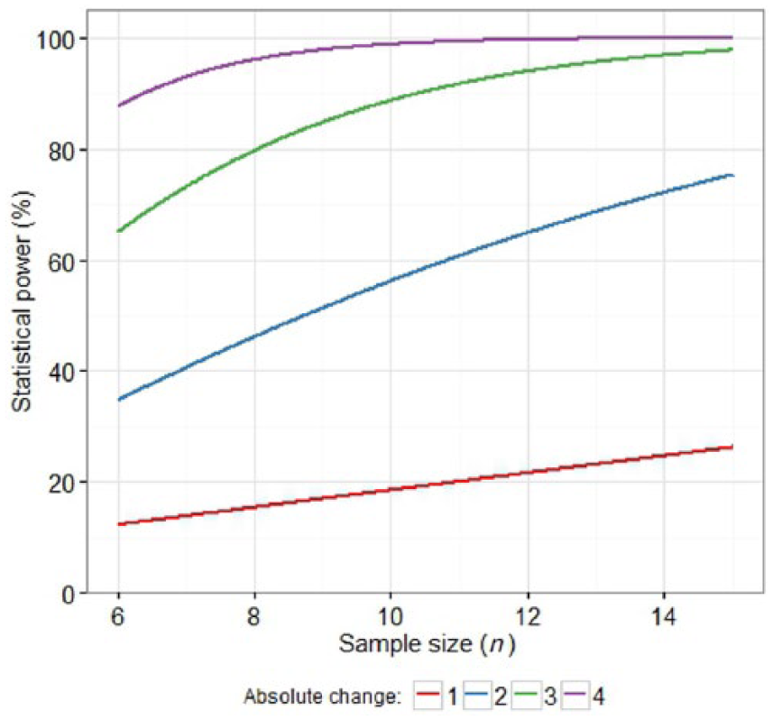
Example of InVivoStat power curves when the standard deviation is 2, the sample size is between two and 10 and the biologically relevant differences range between 1 and 4.

From Figure 2 it can be seen that if the true difference between the treatment and the control is 3 (green line) then, when using six animals per group, the statistical power will be approximately 65%. If the sample size is increased to 10 animals per group, then the statistical power will be approximately 90%.

On avoiding pseudo-replication

Another common problem is pseudo-replication (Ruxton and Colegrave, 2016). This arises when the experimental unit (the smallest unit to which a single level of a treatment can be applied) is measured repeatedly and yet there is no theoretical reason why these measurements might differ, other than from random fluctuations. The experimental designs that are used in such situations are known as nested designs. An example would be when each animal is an experimental unit and a blood sample from each animal is divided into three and assayed in triplicate. Pseudo-replication occurs if every assay measurement is used in the statistical analysis but a factor identifying the animal, from which each measurement is obtained, is not included in the statistical model. Because the treatments are randomly assigned to the experimental units, then their effect needs to be assessed against the variability of the experimental units, and not the (usually smaller) variability of the individual measurements. For example, if ‘Animal’ is the experimental unit, then 20 measurements from the same animal might be expected to be more similar than 20 measurements from 20 different animals.

Such pseudo-replication can easily be avoided if the average of the three measurements for each animal is analysed instead of the individual measurements.

Although it is appropriate to ‘average’ all the measurements collected from each experimental unit, more can be inferred from such data. Such pre-processing of the data produces a more precise estimate of the experimental units’ response and this raises an interesting question regarding the reliability of these ‘average responses’: viz. how many replicate measurements of an experimental unit are needed to obtain suitable precision? More specifically for animal researchers: if we improve the precision of the estimate of each individual animal’s response, by taking an average of repeated measurements, can we reduce the total number of animals used by increasing the within-animal replication?

InVivoStat’s Nested Design Analysis module helps the researcher investigate the levels of replication within a design, for a given estimate of the various sources of variability (i.e. between-animal and within-animal variability). To achieve this, the package calculates the associated statistical power when both the total number of animals and the number of within-animal replicate measurements are varied (Example 4).

It should be noted that nested designs differ from the situation where repeated measurements are indexed by a factor, with different levels, that is shared across all experimental units: so-called repeated measures designs (Bate and Clark, 2014). These apply when a series of measurements is taken from each animal, over time (i.e. Time is a repeated factor in the analysis). In such cases, there may be a known trend across the repeated measurements and the purpose of the analysis is to evaluate this trend.

Example 4: elevated T-maze experiment

An experiment was conducted to investigate the interaction between opioid- and serotonin-mediated neurotransmission in the modulation of defensive responses in rats submitted to the elevated T-maze (Roncon et al., 2014). As part of the experiment, rats were placed at the end of the open arm of the T-maze and the latency to leave this arm was recorded in three consecutive trials. When reviewing the data, there was no effect of trials detected and so the latencies from the three trials (for each animal) were averaged prior to analysis. The experimental treatments were then assessed by considering their effect on these derived averages.

While the primary statistical analysis involves comparing the treatment effects with a control, a secondary analysis could also be performed to investigate the level of within-animal replication in the design. How many repeat trials should be performed using each animal? And can the number of animals used in the study be reduced by increasing the number of trials per animal? These questions can be answered because this is an example of a nested design: animals are ‘nested within treatments’ as each animal receives only one of the treatments and trials are ‘nested within animals’ as each trial is unique to each animal. Such designs can be visualised, as shown in Figure 3.

Figure 3.

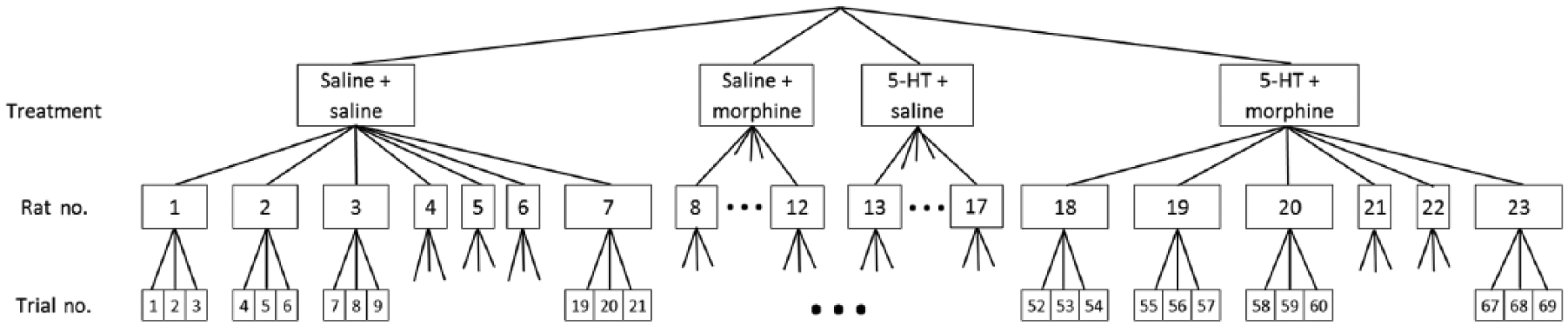
Diagrammatical illustration of the structure of the nested design employed in Example 4 (see also: Roncon et al. (2014), Experiment 2, Table 1).

Using InVivoStat’s Nested Design Analysis module in a simulated experiment (see: Section 6, Supplementary Material), increasing the number of trials per animal from one to three had a larger impact on the statistical power than increasing the number of animals from six to seven (Figure 4).

Figure 4.

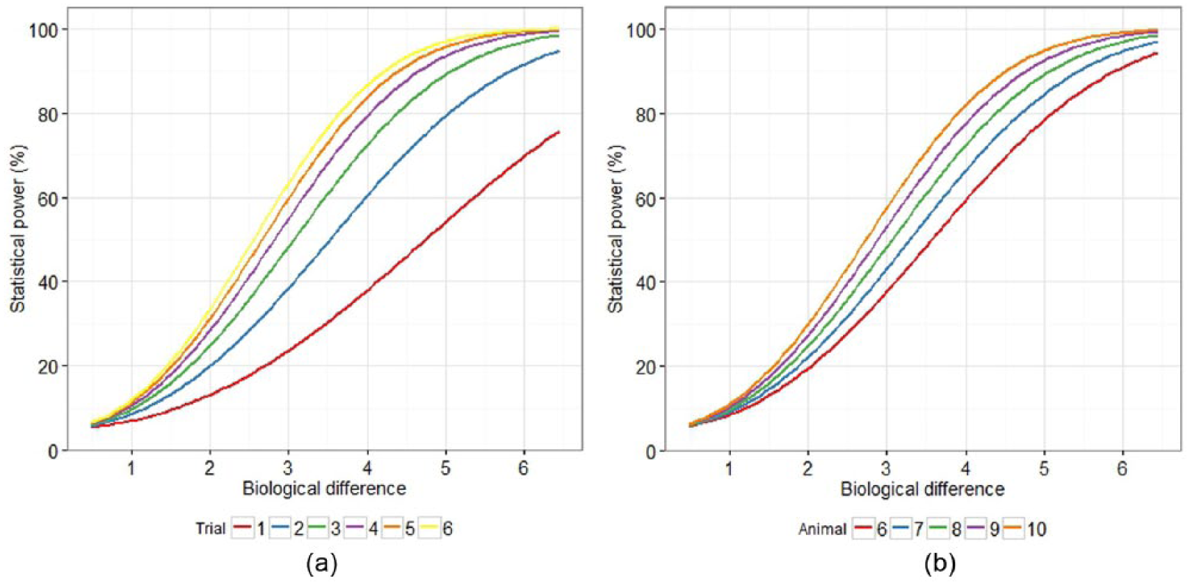
Power curves for varying the number of animals and the number of trials for each animal. (a) Varying the number of trials for each animal from one to six, with eight animals per group. (b) Varying the number of animals from six to 10 per group, with three trials per animal.

In Figure 4(a) the effect of increasing the number of trials from three to four per animal, when the true biological effect is a change in latency of approximately 4 s, increases the statistical power by 10%, at most. Intriguingly, raising the number of animals from six to seven increases the statistical power by a similar amount (Figure 4(b)). From Figure 4(a), it is also clear that there is an increase in power when more than one trial per animal is conducted, implying that at least three trials per animal should be used in future experiments.

Considering alternative approaches in statistical analysis

This section explains how InVivoStat can help researchers decide on what statistical analysis should be used and why some are preferable to others in certain situations.

On performing normalisation

Normalisation is often used to reduce the effect of any within-group variability that exists at baseline: for example, the statistical analysis is performed on the % change from the baseline response. There are certain circumstances when such normalisation is recommended: for instance, when the estimate of the linear best-fit line, linking the post-treatment and baseline responses, passes through the origin. However, the percent change from baseline can introduce, rather than diminish, variability because the amplitude of a percentage change depends on the baseline: that is, two responses that are identical in amplitude could differ greatly, when transformed to percentages, if the baselines differ appreciably. This implies that a percentage response could potentially be a more variable response to analyse because the variability of a percentage response is influenced by both baseline variability and post-treatment response variability.

A more flexible modelling approach, which avoids this problem, is to include the baseline as a covariate in the statistical model. Covariates are continuous responses, usually measured pre-treatment, that can explain some of the post-treatment between-animal variability in the statistical analysis. This approach will account for the within-group variability of the individual baseline values, regardless of the underlying relationship with the response, without increasing the variability of the analysed response. By including a suitable covariate in the statistical model (leading to an analysis of covariance (ANCOVA)), the variability that the effects of interest are tested against is reduced and the statistical tests will be more sensitive.

Many modules within InVivoStat allow the user to include a covariate in the statistical model: for example, the Single Measures Parametric Analysis (SMPA), Repeated Measures Parametric Analysis, and Nested Design Analysis modules.

Certain assumptions are made when fitting covariates: (i) there is a valid reason to predict a correlation between the response and the covariate; (ii) the covariate should not be influenced by the treatment (pre-treatment measures can be assumed to be free of treatment effects); and (iii) the relationship between covariate and response should be the same for all treatment groups. InVivoStat provides users with a plot (e.g. Figure 5) and some contextual guidance to help them decide if it is appropriate to fit the covariate in the statistical model.

Figure 5.

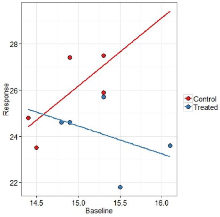
Scatterplot generated as part of InVivoStat analysis of covariance, categorised by the Treatment factor.

Example 5: assessing the effect of phenotype on locomotor activity

An experiment was conducted to assess the effect of a novel treatment on locomotor activity in female mice. Ten mice were randomly assigned to groups (five control and five treated animals). Each mouse was assessed pre- and post-treatment and, following an established protocol, the percent change in response was assessed in the statistical analysis. The percent change was statistically significant (p=0.0467). However, upon further examination of the data, it was discovered that there was little evidence of a correlation between the pre- and post-treatment responses (Pearson’s correlation coefficient = −0.137, p=0.706). Additionally, there was a subtle difference at baseline (despite the randomisation) where animals in the ‘to be treated’ group had higher pre-treatment responses. If, in reality, there is no relationship between pre- and post-treatment responses, then calculating the percent change in the response has artificially reduced the treatment response mean, compared with the control mean. If an ANCOVA analysis had been performed instead, with pre-treatment as a baseline, then it would have been discovered that (i) the pre-treatment responses should not be used to ‘normalise’ the data because they do not predict post-treatment responses and (ii) there is little evidence of a treatment effect in this experiment. Figure 5 is a scatterplot, which is produced by InVivoStat automatically when fitting a covariate: this highlights the lack of correlation between pre- and post-treatment responses. A further description of the analysis of this dataset is given in the Supplementary Material, Section 7.

Another form of normalisation that is often used is to standardise data to the control group mean. Yet, it has been pointed out that this approach ‘gives the false impression that control values … are identical from one experimental data set to another’ (e.g. Curtis et al., 2015). The advantage of covariate analysis is that it implies that the predicted means from the analysis are presented on the original scale and so avoids this issue.

On using transformations

Transformation of the responses is often used to satisfy some of the criteria for valid parametric analysis (e.g. that the variance is homogeneous) and to legitimise their use. This strategy is certainly recommended, especially if the group sizes are relatively small; statistical power can be low if a less powerful (e.g. non-parametric) statistical test is used to analyse the raw data instead. InVivoStat makes it straightforward to apply a transformation by providing a drop-down list of options (including log₁₀, log_e, square root, arcsine and rank) in many of its modules. When a log transformation is applied, certain results can be presented on both the log and the back-transformed scale.

Many journals require evidence to justify performing a transformation. There are statistical tests that can be used to provide such a justification: e.g. Shapiro–Wilk’s test for normality or Levene’s and Bartlett’s tests for equal variance (homogeneity of variance). However, such tests may lack statistical power, especially if the sample sizes are small, and so the need to perform a transformation can be missed. An alternative, graphically-based, approach is to consider the residuals versus predicted plot (Figure 6). This consists of a scatterplot where the x-axis variable represents the ‘predicted’ values (the predictions from the statistical model, i.e. a group mean) and the y-axis variable is the ‘absolute residuals’ (the difference between the actual observation and its predicted value). So for each observation, i, in the dataset:

{Observation}_{i} {= Prediction}_{i} {+ Absolute residual}_{i .}

Figure 6.

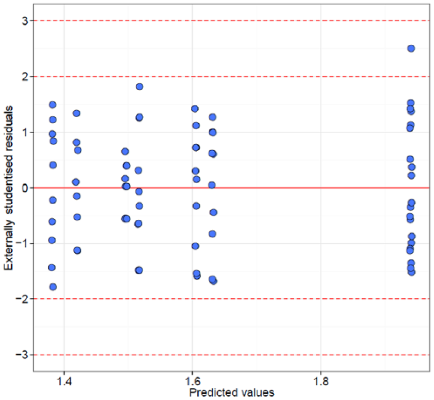
InVivoStat externally studentised residuals versus predicted diagnostic plot.

If the variability is roughly the same across all groups, then the spread of the residuals should be the same for all groups and the dots on the plot should exhibit no patterns or systematic trends. In practice, biological responses can often become more variable as they increase in magnitude and so, when moving from left to right across the residual versus predicted plot, a ‘fanning’ effect will be observed. In this case, a transformation such as the log transformation will be required.

The residuals presented by InVivoStat are defined as externally studentised residuals. To ‘studentise’ a residual, the absolute residual is divided by an estimate of the standard deviation (i.e. the Mean Square Residual in the ANOVA table). Because the scale of the Y-axis of the plot produced by InVivoStat is in standard deviation units, it can be used to test for outliers (the 2SD or 3SD rules, for example, as highlighted by the horizontal dotted lines on the plot). The estimate of the standard deviation used in the studentisation is effectively an average SD (averaged over all the data) and hence could be influenced by an outlier artificially inflating it. To account for this, when estimating the predicted value and studentised residual for a given observation, the observation is first removed from the dataset and the predicted value, variance (and hence studentised residual) are estimated using a dataset excluding the observation. These are defined as the externally studentised residuals. In theory if the observation is an outlier then including it in the dataset implies (i) it will ‘pull’ the statistical model towards it (e.g. biasing the group mean estimate) and (ii) it will inflate the variability estimate. Taken together (i) and (ii) imply the observation is less likely to be identified as an outlier.

These plots not only provide a subtle/sensitive tool to inform a decision on a suitable transformation, but can also be used to ‘justify’ the choice of transformation. In all relevant modules, InVivoStat produces the residuals versus predicted plot and normal probability plot. InVivoStat also gives contextual advice on how to use these plots and what to look for.

On the gateway ANOVA strategy

The gateway ANOVA strategy, sometimes known as ‘providing Fisher’s protection’ to the post-hoc tests, is applied to help avoid false positive results. The argument is that increasing the number of post-hoc tests increases the risk of making a false positive conclusion and so the analysis strategy should take this into account. Despite its popularity in the non-statistical literature, it should be noted that the tests contained within the ANOVA table are ‘overall’ tests: their function is to test whether or not individual group means are ‘different’ from each other. If the experiment consists of several groups that all have the same status in the experiment, then using the test in the ANOVA table to reduce the risk of false positives can be a valid approach. However, in practice, most experimental designs are more complicated. For instance, there could be a group that serves as an active control when making comparisons of a set of doses of a treatment that are ordered on a dose-scale. The tests in the ANOVA table do not use this additional information and hence can be misleading when used as a gateway test.

Example 6: assessing the effect of buprenorphine and naltrexone in mice

This example is based loosely on an experiment reported in Almatroudi et al. (2015) to investigate the effects of buprenorphine and naltrexone on the number of open arm entries by mice in the elevated plus-maze.

The experiment involved a saline control group and three treatment groups: buprenorphine (1 mg/kg), naltrexone (1 mg/kg) and a buprenorphine (1 mg/kg) + naltrexone (1 mg/kg) combined group. There was also an option to include a positive control, diazepam (2 mg/kg), in the experiment. If the within-group variability of this positive control group is the same as the within-group variability of the other groups, then this positive control group can be included in the statistical analysis to increase statistical power. This is because more animals are being used to obtain an estimate of the overall variability.

Figure 7 shows a plot of the simulated data used in this text that reflects the actual findings of the reported study. If the positive control is included in the statistical analysis, using a one-way ANOVA strategy, then the overall test in the ANOVA table is statistically significant (p=0.002). Using the gateway ANOVA approach, it is therefore ‘justified’ to compare the treated groups back to the saline control group. In this case, it may be concluded that the naltrexone group is statistically significant (p=0.015, Planned Comparison). However, if the positive control is not included in the experiment, then the test in the ANOVA table is not statistically significant (p=0.060). The gateway ANOVA approach would dictate that treatments cannot be compared with the saline control. This means that the inclusion (or not) of the positive control in the experimental design determines whether or not the naltrexone and buprenorphine treated groups can be compared with the saline control group. Clearly this is a dubious position to be in.

Figure 7.

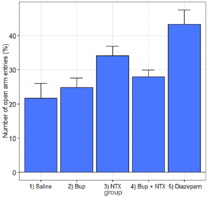
InVivoStat’s observed means with SEM plot for simulated data that reflects the findings of Almatroudi et al. (2015).

An alternative approach is to: (i) generate the unadjusted p-values using, for example, the ‘Unadjusted (LSD)’ post-hoc tests in the Single Measures Parametric Analysis module in InVivoStat (these p-values are not adjusted for the number of comparisons made and hence some could be false positives), (ii) use InVivoStat’s P-Value Adjustment module to perform a multiple comparison adjustment to those comparisons that were planned in advance. Assuming the unadjusted p-values were 0.0184, 0.2019 and 0.5248, then the smallest p-value is no longer statistically significant following adjustment (p=0.0552) (see Section 8.3 of the Supplementary Material).

In an alternative set of circumstances, the reverse scenario to that described in Example 6 could also occur: that is, it is conceivable that a reliable positive control, that appears to have had an effect, is declared non-significant. For example, consider a study conducted to assess several novel treatments that include a positive control and a vehicle control. If none of the novel treatments has an effect, the overall test in the ANOVA table would not be statistically significant. Despite the positive control having a real effect (as expected), this effect is masked in the overall ANOVA test by the non-significance of the novel treatments. If the gateway ANOVA approach is applied in this case then it would lead to the conclusion that the positive control did not have an effect either and that the experiment had failed.

The neglected caveat with both of these scenarios is that there is a structure to the treatments: the positive control has a status in the design that differs from the vehicle control and the novel treatment groups. The ANOVA does not make use of this information and hence the ANOVA test is not appropriate as a ‘gateway’ to the local post-hoc tests.

In our view, if the experiment is well designed and the comparisons decided in advance (the so-called Planned Comparisons) then there is less of a risk of finding a false positive result and no need to use a gateway approach (Armitage et al., 2002). To further reduce the risk of false positives, a more sensible approach is to apply a multiple comparison adjustment (MCA). The SMPA module in InVivoStat offers several different MCAs including Tukey, Bonferroni, Holm, Hochberg, Hommel, Benjamini–Hochberg and Dunnet (when comparing back to a single control group). Within the SMPA module, the adjustments are performed assuming every mean is compared with every other mean (all pairwise tests). However, the size of the adjustment depends on the number of tests that are carried out and so this approach may be too strict. If only some of the ‘all pairwise comparisons’ are needed (i.e. only those that are of scientific interest), then it is advisable to make an adjustment for just that number.

The use of p-values and confidence intervals

The p-value, and the role it plays in a statistical analysis, is often misunderstood. Standard practice is to use it as a test of significance. If p<0.05, for example, then the result is declared ‘statistically significant’ and conversely when p>0.05 the result is declared not significant. When using this strategy, statistics provides a binary result – either it is statistically significant or it is not. In the latter case the researcher may then elaborate on the result, for example commenting that a ‘non-statistically significant’ trend is observed, or ‘the difference was not statistically significant’, even though such statements are oxymorons that indicate subjective bias. In our view, statistics can offer more than just a yes/no decision. Moreover, the real benefit of statistics is that it indicates the confidence researchers can place in their results and conclusions.

The p-value describes the probability of obtaining an experimental result equal to or ‘more extreme’ than the value that was actually observed, given that the null hypothesis (of no effect) is true. The actual numerical p-value therefore contains considerably more information about the experimental result than simply providing a decision on statistical significance: the actual p-value gives a more accurate representation of the evidence that there is a real effect.

Some journals recommend that authors quote only their a priori criterion for significance (usually ‘p<0.05’), rather than specifying the actual p-value (e.g. ‘p=0.044’).The strategy of deciding a priori what level will be deemed statistically significant (i.e. ‘if p<0.05 then the test is significant’) is helpful because this influences the estimate of the statistical power and sample size. However, we contend that this should not prevent the actual p-values being quoted, to three or four decimal places, rather than simply quoting ‘p<0.05’, as this helps readers to judge the strength of the evidence supporting the conclusion. It is also advisable to consider the precision and practical relevance of the observed effects by presenting confidence intervals alongside the p-values. As a component of parametric analyses, InVivoStat produces confidence intervals alongside the comparisons and p-values (Example 7).

Example 7: assessment of active behaviours produced by antidepressants and opioids

Berrocoso et al. (2013) describe an experiment to assess the effect of antidepressants and opioids on active behaviours in the mouse tail suspension test. As part of the investigation, duloxetine (1.25, 2.5, 5, 10, 20, 40 mg/kg) was administered to the mice (8–11 animals per group). Among the responses recorded was the number of times ‘swinging’ was the predominant behaviour in each 5 s period of the 360 s test period. A mouse was judged to be swinging when it continuously moved its paws in the vertical position while keeping its body straight and/or it moved its body from side to side. The statistical analysis involved a one-way ANOVA followed by Dunnett’s test to compare the individual doses back to the control. Statistical significance was indicated by statements such as ‘p<0.05’.

If the analysis had been performed using InVivoStat, then a table containing the absolute differences between the treatments, and also 95% confidence intervals around these differences, would also have been generated. Table 1 contains some simulated results of the experiment. If the user selected the ‘Comparisons back to control’ option in the post-hoc tests, then InVivoStat would also have produced a plot of these differences with 95% confidence intervals (Figure 8).

Table 1.

Plot of all to one comparisons (p-value from Dunnett’s test) with confidence intervals not adjusted for multiple comparisons.

Comparison	Difference	Lower95% CI	Upper95% CI	Standard error	p-value
‘1.25’ vs. ‘0’	13.150	−9.316	35.616	11.223	0.6891
‘2.5’ vs. ‘0’	8.350	−14.116	30.816	11.223	0.9361
‘5’ vs. ‘0’	9.913	−12.553	32.378	11.223	0.8741
‘10’ vs. ‘0’	29.695	8.818	50.573	10.430	0.0292
‘20’ vs. ‘0’	28.714	7.836	49.591	10.430	0.0369
‘40’ vs. ‘0’	27.650	6.772	48.528	10.430	0.0474

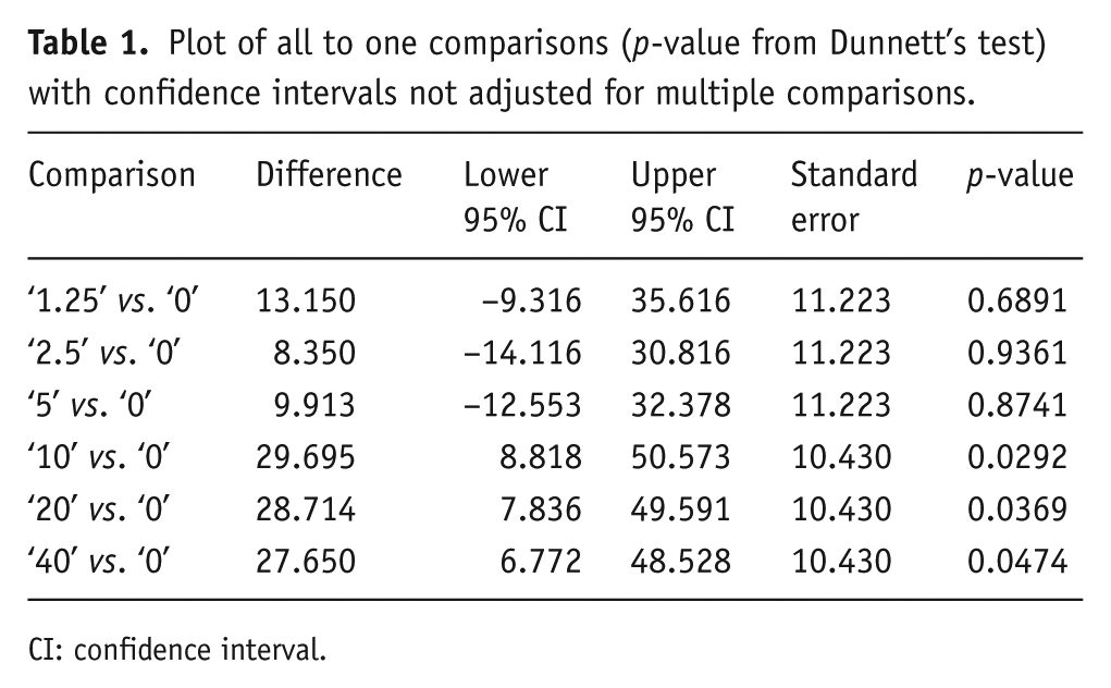
CI: confidence interval.

Figure 8.

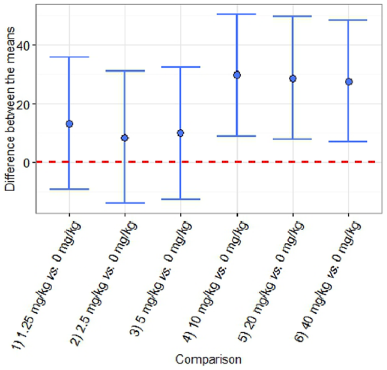
Plot of the mean differences between the responses to increasing doses of the treatment versus control, together with their 95% confidence intervals.

Within InVivoStat, confidence intervals are also given for predicted means from the parametric analyses, observed means in the Summary Statistics module, parameter estimates in the Dose–Response Analysis module and predicted number of events in the Survival Analysis module.

Conclusion

The statistical pitfalls and principles, outlined above, are highly relevant to the design and analysis of the types of experiments carried out by in vivo psychopharmacologists. Here we explain how to avoid some of these problems, particularly when using InVivoStat, to carry out the statistical analysis.

InVivoStat is a free to download statistical package, based on the R statistical language (R Development Core Team, 2013), that was devised to optimise the statistical analysis of animal experiments, such as those reported in this journal. In this paper we offer guidance on the use of statistical analysis modules within InVivoStat that cover the majority of analyses that any biomedical researcher might require. These modules implement analysis tools, such as t-tests, ANOVA, ANCOVA and repeated measures mixed models. InVivoStat can also be used to estimate suitable sample sizes and to provide the information needed to answer more complex questions, such as what is an appropriate level of within-animal replication.

InVivoStat also provides advice on how to check that the assumptions made during the analysis are valid and includes the powerful statistical tools that are needed to ensure that the analysis uses all the information obtained from the experiment. This not only helps to generate more reliable results and conclusions, but can contribute to the 3Rs by reducing excessive use of animals and preventing flawed experimental designs.

Footnotes

Acknowledgements

The authors would like to acknowledge the support of Sarah Channing-Wright (British Association for Psychopharmacology) for her work on the update to the InVivoStat website. We would also like to thank the referees for their insightful comments. In his role as InVivoStat co-developer, STB substantially contributed to the drafting and revising of the article and the ﬁnal approval of the version to be submitted; SCS and RAC revised the article critically for important intellectual content and the ﬁnal approval of the version to be submitted.

Declaration of conflicting interests

The author(s) declared the following potential conflicts of interest with respect to the research, authorship, and/or publication of this article: STB is currently an employee of GlaxoSmithKline Pharmaceuticals. RAC is currently an employee of Envigo Ltd.

Funding

The author(s) received no financial support for the research, authorship, and/or publication of this article: This research received no specific grant from any funding agency in the public, commercial, or not-for-profit sectors.

References

Almatroudi

Husbands

Bailey

. (2015) Combined administration of buprenorphine and naltrexone produces antidepressant-like effects in mice. J Psychopharmacol 29: 812–821.

Armitage

Berry

Matthews

JNS

(2002) Statistical Methods in Medical Research, 4th ed. Malden, MA: Wiley-Blackwell.

Aylott

Bate

Collins

. (2011) Review of the statistical analysis of the dog telemetry study. Pharm Stat 10: 236–249.

Baker

Lidster

Sottomayor

. (2014) Two years later: Journals are not yet enforcing the ARRIVE guidelines on reporting standards for pre-clinical animal studies. PLoS Biol 12: e1001756.

Bate

Clark

(2014) The Design and Statistical Analysis of Animal Experiments. Cambridge, UK: Cambridge University Press.

Berrocoso

Ikeda

Sora

. (2013) Active behaviours produced by antidepressants and opioids in the mouse tail suspension test. Int J Neuropsychopharmacol 16: 151–162.

Borsini

Bordi

Poggi

. (2015) Effects of ST1936, a selective serotonin-6 agonist, on electrical activity of putative mesencephalic dopaminergic neurons in the rat brain. J Psychopharmacol 29: 802–811.

Button

Ioannidis

JPA

Mokrysz

. (2013) Power failure: Why small sample size undermines the reliability of neuroscience. Nat Rev Neurosci 14: 365–376.

Clark

Shoaib

Hewitt

. (2012) A comparison of InVivoStat with other statistical software packages for analysis of data generated from animal experiments. J Psychopharmacol 26: 1136–1142.

10.

Curtis

Bond

Spina

. (2015) Experimental design and analysis and their reporting: New guidance for publication in BJP. Br J Pharmacol 172: 2671–2674.

11.

Festing

MFW

Overend

Gaines Das

. (2002) The Design of Animal Experiments: Reducing the use of Animals in Research through Better Experimental Design. London: Royal Society of Medicine Press.

12.

Gore

Stanley

(2015) Helping to drive the robustness of preclinical research – the assay capability tool. Pharmacol Res Perspect 3: e00162.

13.

Kilkenny

Browne

Cuthill

. (2010) Improving bioscience research reporting: The ARRIVE guidelines for reporting animal research. PLoS Biol 8: e1000412.

14.

Kilkenny

Parsons

Kadyszewski

. (2009) Survey of the quality of experimental design, statistical analysis and reporting of research using animals. PLoS ONE 4: e7824.

15.

Liao

JJZ

Liu

(2009) Re-parameterisation of five-parameter logistic function. J Chemometr 23: 248–253.

16.

McGrath

Lilley

(2015) Implementing guidelines on reporting research using animals (ARRIVE etc.): New requirements for publication in BJP. Br J Pharmacol 172: 3189–3193.

17.

Macleod

Fisher

O’Collins

. (2009) Reprint: Good laboratory practice. Preventing introduction of bias at the bench. J Cereb Blood Flow Metab 29: 221–223.

18.

Macleod

McLean

Kyriakopoulou

. (2015) Risk of bias in reports of in vivo research: A focus for improvement. PLoS Biol 13: e1002273.

19.

Nature Editorial (2014) Journals unite for reproducibility. Nature 515: 7.

20.

Peers

South

Ceuppens

. (2014) Can you trust your animal study data? Nat Rev Drug Discov 13: 560.

21.

R Development Core Team (2013) R: A language and environment for statistical computing. R Foundation for Statistical Computing, Vienna, Austria. Available at: http://www.R-project.org (accessed 16 January 2016).

22.

Roncon

Biesdorf

Coimbra

. (2014) Cooperative regulation of anxiety and panic-related defensive behaviors in the rat periaqueductal grey matter by 5-HT1A and μ-receptors. Psychopharmacology 28: 1155–1160.

23.

Ruxton

Colegrave

(2016) Experimental design for the life sciences. Oxford: Oxford University Press.

24.

Selwyn

(1996) Principles of Experimental Design for the Life Sciences. Boca Raton, USA: CRC Press.

25.

Shoaib

Sidhpura

Shafait

(2003) Investigating the actions of bupropion on dependence-related effects of nicotine in rats. Psychopharmacology 165: 405–412.

26.

U.S. National Institutes of Health (2014) Principles and guidelines for reporting preclinical research. Available at: http://www.nih.gov/about/reporting-preclinical-research.htm (accessed 23 January 2016).

Supplementary Material

Please find the following supplemental material available below.

For Open Access articles published under a Creative Commons License, all supplemental material carries the same license as the article it is associated with.

For non-Open Access articles published, all supplemental material carries a non-exclusive license, and permission requests for re-use of supplemental material or any part of supplemental material shall be sent directly to the copyright owner as specified in the copyright notice associated with the article.

0.00 MB

1.11 MB