Similarity Indices for 500 Classical Music Composers

Abstract

In a recent article the authors inferred classical composer similarities on the basis of their common and distinct personal (individual) musical influences. In this paper, the authors examine how much, if any, additional explanation can be added when ‘ecological’ measures (i.e., other characteristics such as time period, geographical location, school association, instrumentation emphases, etc.) are also taken into account. Although the two methods do not generate identical similarities rankings, their combination does provide, arguably, an improved system of ranking.

Keywords

classical music classical composers composer influences measures of association similarity indices

Introduction: Composer Similarities

Charles H. Smith created The Classical Music Navigator (Smith, 2000; hereafter referred to as CMN) as a combined reference work and experiment in music education (see Smith & Georges, 2014 for a review of the philosophy and methodology underlying the CMN). The core of the CMN approach is the collection of composer-related data: specifically, on composer influences, and on various secondary form and style characteristics (later referred to as ‘ecological’ characteristics). The personal influences part of the database consists of, for each of the 500 composers treated, those other composers identified to have had an influence on their work. Smith and Georges (2014) used these data to infer degrees of similarity among the 500 composers and proposed the use of three similarities indices (in an approach akin to biosystematic analyses of biotas or phylogenetic relations) by means of pairwise comparison of presence–absence data (i.e., in analogy to presence–absence of characters within a group of taxonomic units, or of regional units in a spatial, biogeographic, sense). Note was taken that a second collection of data in the CMN associates each of the 500 composers with characteristics such as time period, geographical location, school association, instrumentation emphases, and so forth depicted for convenience here as ‘ecological categories’. In this new paper, we group the latter from the CMN into 298 variable categories (see Appendix for a list) with the objective of examining how much, if any, additional explanation can be added through them to the personal influences-based rankings of similarity.

To illustrate, Figure 1 focuses on three composers in the CMN. Figure 1(a) diagrams all composers flagged in the CMN as having influenced Joseph Haydn, Wolfgang Amadeus Mozart, and Franz Schubert. These three Austrian composers, born, respectively, in 1732, 1756, and 1792, are typically associated with the Classical Period of Western classical music. Even a casual listening suggests style similarities across them, although to most ears Haydn and Mozart would probably sound ‘closer’ than Haydn and Schubert, or Mozart and Schubert.¹ Observe in Figure 1(a) that these three composers share in common two particular influences: Handel and Gluck. But the important characteristic to notice is that the number of shared influences fluctuates between pairs. For example, besides Handel and Gluck, there are no further common influences between Schubert and Haydn; there are, however, two additional common influences between Schubert and Mozart (M. Haydn and J. S. Bach) and five additional common influences between Haydn and Mozart (Fux, Hasse, C. P. E. Bach, G. B. Sammartini, and J. Stamitz). Our contention is that the greater number of common personal influences between Haydn and Mozart is likely to be reflected in a tighter proximity of the musical styles of these two composers as compared with the styles of Schubert and Mozart, let alone of Schubert and Haydn. Figure 1(b) presents a similar message with respect to some (there unnamed) ecological categories that might be used to characterize a composer. Eight categories are associated with all three composers, reflecting an overall similarity of these three Austrian Classical Period composers in terms of their sharing a particular spatial-temporal musical niche. However, Haydn and Mozart share nine additional ecological categories, while Haydn and Schubert share just one additional ecological category, and Mozart and Schubert share five additional ones. In this case, therefore, the ecological categories data seem to corroborate the personal influences data, again pointing to a greater similarity of Haydn and Mozart.

Figure 1.

(a) Composer personal influences network—J. Haydn, W. A. Mozart, and Schubert. (b) Composer ecological categories network—J. Haydn, W. A. Mozart, and Schubert.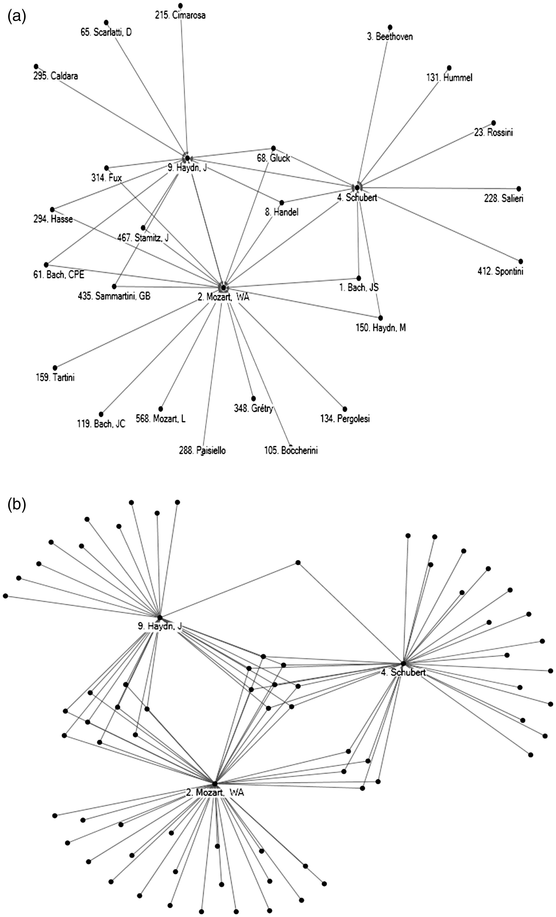

Even if shared personal influences and common ecological categories tend to reflect similarities in the compositional style of composers, distinct personal influences and ecological categories may yet increase the distance between the musical styles of any pair of composers. For example, as shown in Figure 1(a), Schubert has five musical influences that he does not share with Mozart (Beethoven, Hummel, Rossini, Salieri, and Spontini), while Mozart has 12 distinct influences that he does not share with Schubert (Fux, Hasse, J. Stamitz, C. P. E. Bach, J. C. Bach, Grétry, Tartini, Paisiello, Boccherini, Pergolesi, L. Mozart, and G. B. Sammartini). Additionally, although Schubert and Mozart share 13 ecological categories (Figure 1(b)), Schubert can be characterized by 18 additional categories that do not characterize Mozart, while Mozart has 30 additional categories that do not characterize Schubert—ultimately speaking to probable differences between the musical oeuvres of the two composers. The same argument can be made of the relative proximity of Debussy and Ravel when compared with Bartók in Figure 2(a) and (b), on the basis of shared and distinct personal influences and ecological categories between pairs of composers. Thus, to recap, our theory is that although common personal influences and ecological categories tend to reflect (or even explain) style similarities between pair of composers, distinct influences and ecological categories should have the opposite effect of increasing the distance (i.e., reflecting greater differences) between musical styles of composers.

Figure 2.

(a) Composer personal influences network—Debussy, Ravel, and Bartók. (b) Composer ecological categories network—Debussy, Ravel, and Bartók.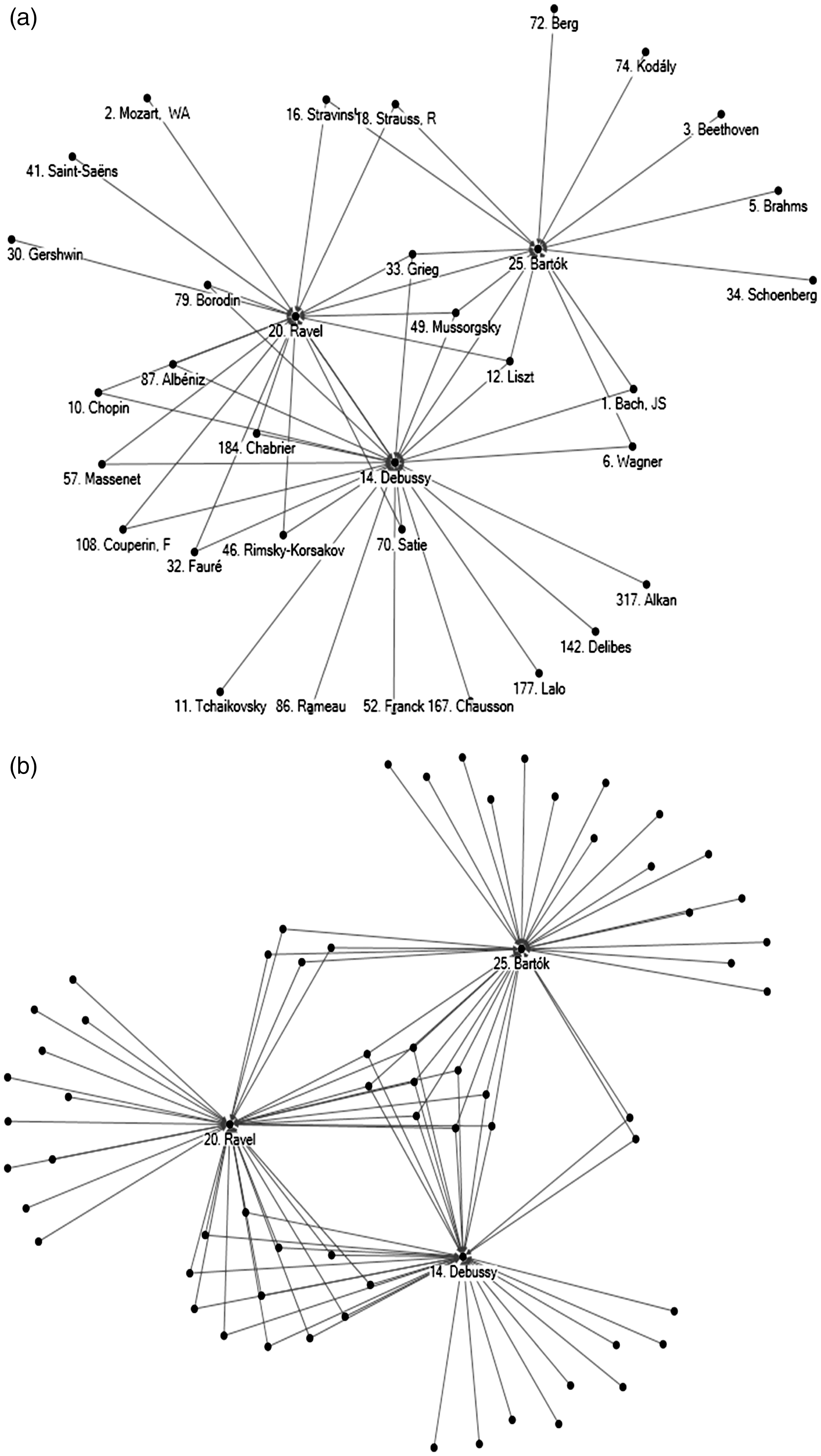

Although an inspection of diagrams such as Figures 1 and 2 is useful to visualizing relative similarities among the composers, Smith and Georges (2014) also developed a method for generating similarity scores between any pair of composers, based on these common and distinct personal influences. This is reminiscent of the approaches used in biodiversity analyses to identify relational patterns useful to explaining the historical evolution of the forms under study. See Cheetham and Hazel (1969) and Hayek (1994) for good surveys of such studies, and the related ‘measures of association’ (also named in a somewhat interchangeable way ‘similarity’, ‘resemblance’, or ‘matching’ indices). Dozens of measures of association have been constructed and applied in the biosystematics literature, and after an investigation of some of their relative qualities, Smith and Georges (2014) decided to concentrate on three specific similarity indices to link pairings of composers i and j included in the database of 500 composers: the Jaccard (1901) index, the Smith (1983) index, and the binomial index of dispersion (Potthoff & Whittinghill, 1966).

In this new paper, we explore the robustness of our earlier results by attempting to infer composer similarities on the basis of ecological categories, instead of personal influences. We further propose combining the ecological and personal influences to assess similarities, arguing that this should produce a general improvement in the similarity rankings.

Methods

The analysis methods for this new study are essentially the same as those reported in Smith and Georges (2014). In that work, C is the set of 500 composers in the database, and for any pair of composers (i,j) for $i, j \in C$ (among the 500 × 500 possible pairs), we are interested in capturing whether a composer $k \in C$ had a reported influence in the CMN on both i and j, on i but not j, on j but not i, and on neither i nor j. Running this across the 500 composers k for each pair (i,j), we eventually obtain the set I_i of all composers who influenced composer i, and the set I_j of all composers who influenced j. Also, for any pair (i,j), $I_{i} \cap I_{j} = {CI}_{i, j}$ is the set of composers k that influenced both i and j; $I_{i} - I_{i} \cap I_{j} = I_{i, - j}$ is the set of composers k that influenced i but not j; $I_{j} - I_{i} \cap I_{j} = I_{j, - i}$ is the set of composers k that influenced j but not i, and ${DI}_{i, j} = I_{i, - j} \cup I_{j, - i}$ is the set of composers k that influenced either i or j but not both. These tallies produce a count table for the pair (i,j) that sums the elements (the number of composers k) in each of the four sets ${CI}_{i, j}$ , $I_{i, - j}$ , $I_{j, - i}$ , and $C - {CI}_{i, j} - {DI}_{i, j}$ , and from which a similarity index for the pair of composers (i, j) can be computed on the basis of well-known formulas (e.g., the Jaccard index, etc.—see formulas and respective interpretation in Smith and Georges, 2014). In what follows, we report only the results obtained using the binomial index of dispersion, as this arguably provides the generally most useful kinds of results and is based on the $χ^{2}$ statistic (see Smith & Georges, 2014 for further information). This similarity index can be computed for any pair (i,j) as: ${SI}_{i, j} |_{BID} = n (ad - bc) 2 / [(a + b) (c + d) (a + c) (b + d)]$ where a, b, c, d, and n are the count/number of composers in each of the five sets ${CI}_{i, j}$ , $I_{i, - j}$ , $I_{j, - i}$ , $C - {CI}_{i, j} - {DI}_{i, j}$ , and C. Eventually, this method generates 250,000 similarity indices, one for each of the 500 × 500 pairings of composers (i,j).

The methodology with respect to the set of 298 ecological categories, E, given in Appendix, is similar. This time, however, we are interested in capturing whether an ecological category $e \in E$ is part of the musical ecological niche (as reported in the CMN Index of Forms and Styles of Music) of both i and j, of i but not j, of j but not i, and of neither i nor j. Tallying these across the 298 ecological categories e for any pair of composers (i,j), and following the method above, we generate a count table that permits the calculation of a similarity score for the pair of composers (i,j) based, this time, on the ecological categories.² Eventually, we arrive at a second set of 250,000 similarity indices, one for each of the 500 × 500 pairs of composers (i,j).

Finally, for the analysis combining personal influences and ecological categories, we want to capture whether a composer $k \in C$ has an influence on both i and j, on i but not j, and so forth and whether an ecological category $e \in E$ is part of the musical ecological niche of both i and j, of i but not j, and so forth. Doing this across the 500 composers k and the 298 ecological categories e for any pair of composers (i,j), we again generate a count table that leads to a similarity index for the pair of composer (i,j) based on the cumulative information given by personal influences and ecological categories.³ When repeating for all pairs of composers, a third and final set of 250,000 integrated similarities scores emerges.

Results

Selecting the 20 most significant composers (according to the CMN), Tables 1 to 3 identify these composers’ intersimilarities. The index values given are the χ² statistics produced through the binomial index of dispersion. Table 1 reports the results based on the personal influences data, while Table 2 is based on the ecological categories, and Table 3 is based on the combination of personal and ecological categories. Results are roughly in line with our priors. For example, in Table 1, Ravel is the most similar composer to Debussy, or Haydn is the most similar composer to Mozart and Mahler the most similar to R. Strauss. Thus, the results tend to strengthen our earlier observations that Mozart and Haydn are more similar than are Mozart and Schubert, let alone Haydn and Schubert. Of course, even if Puccini is reported (among this list of 20 composers) as being most similar to Stravinsky, it does not necessarily mean that Puccini’s style is so very similar to Stravinsky’s. A search among all of the 500 composers (instead of just these 20) would identify the one most similar composer to Stravinsky (as is done in Tables 4 to 6 for the top 10 names in the list), as measured here.

Table 1.

Composer Similarities Index—Personal Influences Database (Chi-square Statistics From the Binomial Index of Dispersion; Potthoff and Whittinghill, 1966).

	1. Bach	2. Mozart	3. Beethoven	4. Schubert	5. Brahms	6. Wagner	7. Verdi	8. Handel	9. Haydn	10. Chopin
1. Bach, JS	500.00	2.58	2.58	0.59	16.68	0.02	0.76	40.59	5.08	0.61
2. Mozart, WA	2.58	500.00	62.78	64.83	12.90	3.11	0.34	0.41	132.62	0.87
3. Beethoven	2.58	62.78	500.00	95.73	62.78	31.96	1.52	0.41	95.73	32.75
4. Schubert	0.59	64.83	95.73	500.00	64.83	74.83	15.03	0.28	32.86	81.57
5. Brahms	16.68	12.90	62.78	64.83	500.00	48.31	1.52	1.05	21.04	53.57
6. Wagner	0.02	3.11	31.96	74.83	48.31	500.00	83.33	0.51	5.89	86.36
7. Verdi	0.76	0.34	1.52	15.03	1.52	83.33	500.00	0.25	0.23	56.36
8. Handel	40.59	0.41	0.41	0.28	1.05	0.51	0.25	500.00	2.15	0.33
9. Haydn, J	5.08	132.62	95.73	32.86	21.04	5.89	0.23	2.15	500.00	10.78
10. Chopin	0.61	0.87	32.75	81.57	53.57	86.36	56.36	0.33	10.78	500.00
11. Tchaikovsky	0.71	0.51	0.60	8.91	27.49	52.19	25.56	0.38	1.43	7.03
12. Liszt	0.06	0.33	36.41	56.78	54.73	79.54	63.30	0.46	0.98	97.10
13. Schumann, R	0.47	1.52	1.52	36.65	106.28	56.23	3.33	0.25	0.23	132.76
14. Debussy	0.00	0.13	0.13	0.59	8.09	5.56	0.76	0.57	0.52	0.34
15. Puccini	0.71	0.51	0.60	1.43	0.60	3.51	10.13	0.38	1.43	1.01
16. Stravinsky	0.81	0.41	4.17	7.48	4.17	8.54	0.36	0.43	1.11	15.73
17. Mendelssohn	3.83	32.75	110.52	119.84	79.50	86.36	12.20	0.33	27.04	138.41
18. Strauss, R	0.34	0.44	0.87	1.87	32.75	24.91	12.20	0.33	1.87	1.37
19. Mahler	0.52	1.26	8.15	32.86	64.83	74.83	36.65	0.28	2.48	50.63
20. Ravel	0.06	0.62	0.33	0.98	10.93	7.80	0.38	0.46	0.98	0.64
1. Bach, JS	0.71	0.06	0.47	0.00	0.71	0.81	3.83	0.34	0.52	0.06
2. Mozart, WA	0.51	0.33	1.52	0.13	0.51	0.41	32.75	0.44	1.26	0.62
3. Beethoven	0.60	36.41	1.52	0.13	0.60	4.17	110.52	0.87	8.15	0.33
4. Schubert	8.91	56.78	36.65	0.59	1.43	7.48	119.84	1.87	32.86	0.98
5. Brahms	27.49	54.73	106.28	8.09	0.60	4.17	79.50	32.75	64.83	10.93
6. Wagner	52.19	79.54	56.23	5.56	3.51	8.54	86.36	24.91	74.83	7.80
7. Verdi	25.56	63.30	3.33	0.76	10.13	0.36	12.20	12.20	36.65	0.38
8. Handel	0.38	0.46	0.25	0.57	0.38	0.43	0.33	0.33	0.28	0.46
9. Haydn, J	1.43	0.98	0.23	0.52	1.43	1.11	27.04	1.87	2.48	0.98
10. Chopin	7.03	97.10	132.76	0.34	1.01	15.73	138.41	1.37	50.63	0.64
11. Tchaikovsky	500.00	59.04	10.13	30.78	48.90	4.65	7.03	35.37	69.66	39.39
12. Liszt	59.04	500.00	171.63	6.68	11.98	10.01	97.10	28.39	154.87	3.04
13. Schumann, R	10.13	171.63	500.00	5.90	0.32	8.56	90.53	2.21	67.76	1.20
14. Debussy	30.78	6.68	5.90	500.00	18.23	26.17	0.34	11.07	13.99	172.11
15. Puccini	48.90	11.98	0.32	18.23	500.00	42.19	1.01	7.03	8.91	59.04
16. Stravinsky	4.65	10.01	8.56	26.17	42.19	500.00	15.73	0.75	19.52	33.79
17. Mendelssohn	7.03	97.10	90.53	0.34	1.01	15.73	500.00	1.37	50.63	0.64
18. Strauss, R	35.37	28.39	2.21	11.07	7.03	0.75	1.37	500.00	165.46	14.59
19. Mahler	69.66	154.87	67.76	13.99	8.91	19.52	50.63	165.46	500.00	6.89
20. Ravel	39.39	3.04	1.20	172.11	59.04	33.79	0.64	14.59	6.89	500.00

Note. Tables 1 to 3 and 4 to 6 should be read vertically (column-wise). For example, in Table 1, when considering which composer from among these top-20 figures is the most similar to Debussy (identified in Column 14), we observe that the highest similarity statistic lies opposite Ravel (identified in Row 20). This value, 172.11, is shaded in gray. These relations need not be, and usually are not, symmetrical. For example, among the top-20 composers, Schumann is the most similar to Brahms (106.28), but Liszt, not Brahms, is the most similar to Schumann (171.63), even if the ‘distance’ (similarity) between Schumann and Brahms is the same as the one between Brahms and Schumann (106.28). Finally, note that where a tie occurs, two (or more) cells are shaded in the same column (as in Column 5 in Table 2, where both Mendelssohn and Liszt are identified as equally similar [46.34] to Brahms).

Table 2.

Composer Similarities Index—Ecological Categories Database (Chi-square Statistics From the Binomial Index of Dispersion; Potthoff and Whittinghill, 1966).

	1. Bach	2. Mozart	3. Beethoven	4. Schubert	5. Brahms	6. Wagner	7. Verdi	8. Handel	9. Haydn	10. Chopin
1. Bach, JS	298.00	3.96	1.86	0.01	0.38	0.05	2.08	48.26	9.74	1.26
2. Mozart, WA	3.96	298.00	36.19	21.20	5.92	0.02	4.45	11.09	53.62	1.21
3. Beethoven	1.86	36.19	298.00	58.85	15.82	7.22	16.59	2.02	47.38	13.41
4. Schubert	0.01	21.20	58.85	298.00	13.76	0.04	15.06	0.24	15.67	1.02
5. Brahms	0.38	5.92	15.82	13.76	298.00	3.91	16.01	2.48	1.53	1.45
6. Wagner	0.05	0.02	7.22	0.04	3.91	298.00	26.43	1.20	0.85	5.69
7. Verdi	2.08	4.45	16.59	15.06	16.01	26.43	298.00	1.62	4.29	0.24
8. Handel	48.26	11.09	2.02	0.24	2.48	1.20	1.62	298.00	26.33	2.56
9. Haydn, J	9.74	53.62	47.38	15.67	1.53	0.85	4.29	26.33	298.00	1.44
10. Chopin	1.26	1.21	13.41	1.02	1.45	5.69	0.24	2.56	1.44	298.00
11. Tchaikovsky	0.11	0.84	10.89	5.98	36.93	6.83	8.72	0.18	0.01	7.45
12. Liszt	0.00	0.02	2.93	17.92	46.34	8.55	10.96	0.02	0.15	33.27
13. Schumann, R	0.53	6.55	34.79	31.35	24.59	6.83	0.83	0.03	0.61	27.25
14. Debussy	1.01	0.54	3.32	5.06	9.24	1.74	0.03	0.30	1.63	17.43
15. Puccini	1.31	0.00	2.90	0.12	1.33	18.39	57.61	1.02	0.20	0.98
16. Stravinsky	3.95	0.07	1.61	0.02	0.02	1.88	0.74	0.01	0.00	1.02
17. Mendelssohn	1.27	3.60	34.41	39.06	46.34	17.59	19.35	0.23	3.24	1.80
18. Strauss, R	0.43	0.40	2.61	2.10	36.31	16.72	1.15	0.16	1.02	0.16
19. Mahler	2.68	0.63	0.11	24.71	23.30	7.57	13.00	2.08	0.41	0.06
20. Ravel	3.06	0.37	10.87	13.26	9.74	1.29	0.10	0.63	0.14	9.15
1. Bach, JS	0.11	0.00	0.53	1.01	1.31	3.95	1.27	0.43	2.68	3.06
2. Mozart, WA	0.84	0.02	6.55	0.54	0.00	0.07	3.60	0.40	0.63	0.37
3. Beethoven	10.89	2.93	34.79	3.32	2.90	1.61	34.41	2.61	0.11	10.87
4. Schubert	5.98	17.92	31.35	5.06	0.12	0.02	39.06	2.10	24.71	13.26
5. Brahms	36.93	46.34	24.59	9.24	1.33	0.02	46.34	36.31	23.30	9.74
6. Wagner	6.83	8.55	6.83	1.74	18.39	1.88	17.59	16.72	7.57	1.29
7. Verdi	8.72	10.96	0.83	0.03	57.61	0.74	19.35	1.15	13.00	0.10
8. Handel	0.18	0.02	0.03	0.30	1.02	0.01	0.23	0.16	2.08	0.63
9. Haydn, J	0.01	0.15	0.61	1.63	0.20	0.00	3.24	1.02	0.41	0.14
10. Chopin	7.45	33.27	27.25	17.43	0.98	1.02	1.80	0.16	0.06	9.15
11. Tchaikovsky	298.00	18.96	14.64	5.52	8.51	1.40	50.17	23.85	2.09	14.19
12. Liszt	18.96	298.00	25.37	16.94	0.28	0.76	50.11	22.58	31.43	13.62
13. Schumann, R	14.64	25.37	298.00	12.91	0.14	0.50	25.37	4.85	10.67	14.19
14. Debussy	5.52	16.94	12.91	298.00	7.72	5.06	2.14	21.42	4.87	96.77
15. Puccini	8.51	0.28	0.14	7.72	298.00	2.54	3.55	3.31	1.47	6.39
16. Stravinsky	1.40	0.76	0.50	5.06	2.54	298.00	0.76	0.62	0.17	23.10
17. Mendelssohn	50.17	50.11	25.37	2.14	3.55	0.76	298.00	11.03	13.44	9.37
18. Strauss, R	23.85	22.58	4.85	21.42	3.31	0.62	11.03	298.00	41.22	12.63
19. Mahler	2.09	31.43	10.67	4.87	1.47	0.17	13.44	41.22	298.00	7.73
20. Ravel	14.19	13.62	14.19	96.77	6.39	23.10	9.37	12.63	7.73	298.00

Table 3.

Composer Similarities Index—Integration of Personal Influences and Ecological Categories (Chi-square Statistics From the Binomial Index of Dispersion; Potthoff and Whittinghill, 1966).

	1. Bach	2. Mozart	3. Beethoven	4. Schubert	5. Brahms	6. Wagner	7. Verdi	8. Handel	9. Haydn	10. Chopin
1. Bach, JS	798.00	14.92	8.06	1.89	4.16	0.07	0.39	120.96	26.04	1.08
2. Mozart, WA	14.92	798.00	107.43	81.43	26.42	0.47	4.28	22.29	175.57	3.91
3. Beethoven	8.06	107.43	798.00	163.96	67.48	28.68	21.32	4.28	143.01	44.93
4. Schubert	1.89	81.43	163.96	798.00	64.04	22.67	34.08	0.08	53.50	28.64
5. Brahms	4.16	26.42	67.48	64.04	798.00	27.34	22.30	0.08	15.70	24.55
6. Wagner	0.07	0.47	28.68	22.67	27.34	798.00	98.63	0.05	0.32	64.61
7. Verdi	0.39	4.28	21.32	34.08	22.30	98.63	798.00	1.41	4.10	23.96
8. Handel	120.96	22.29	4.28	0.08	0.08	0.05	1.41	798.00	52.61	2.04
9. Haydn, J	26.04	175.57	143.01	53.50	15.70	0.32	4.10	52.61	798.00	9.30
10. Chopin	1.08	3.91	44.93	28.64	24.55	64.61	23.96	2.04	9.30	798.00
11. Tchaikovsky	0.01	2.46	18.48	20.77	88.48	38.31	31.09	0.02	1.64	18.34
12. Liszt	0.48	1.07	25.55	65.86	115.64	63.53	57.73	0.04	1.77	118.41
13. Schumann, R	2.27	19.07	57.10	87.77	103.41	33.83	3.90	1.09	2.37	113.59
14. Debussy	0.09	2.62	5.84	10.60	25.03	5.66	0.26	0.03	2.38	19.57
15. Puccini	2.11	0.27	2.72	0.66	1.44	14.39	53.61	1.48	0.86	1.78
16. Stravinsky	2.72	0.68	7.68	2.72	2.21	7.20	0.47	0.43	1.30	10.78
17. Mendelssohn	7.56	25.94	126.49	137.50	134.84	73.87	37.54	1.21	21.54	54.26
18. Strauss, R	0.12	1.60	6.93	8.01	90.99	33.83	8.92	1.09	5.25	1.63
19. Mahler	2.40	0.01	1.96	62.46	78.30	61.88	45.99	1.69	2.81	18.81
20. Ravel	0.65	0.00	18.06	26.51	30.81	5.66	0.14	0.03	2.38	13.56
1. Bach, JS	0.01	0.48	2.27	0.09	2.11	2.72	7.56	0.12	2.40	0.65
2. Mozart, WA	2.46	1.07	19.07	2.62	0.27	0.68	25.94	1.60	0.01	0.00
3. Beethoven	18.48	25.55	57.10	5.84	2.72	7.68	126.49	6.93	1.96	18.06
4. Schubert	20.77	65.86	87.77	10.60	0.66	2.72	137.50	8.01	62.46	26.51
5. Brahms	88.48	115.64	103.41	25.03	1.44	2.21	134.84	90.99	78.30	30.81
6. Wagner	38.31	63.53	33.83	5.66	14.39	7.20	73.87	33.83	61.88	5.66
7. Verdi	31.09	57.73	3.90	0.26	53.61	0.47	37.54	8.92	45.99	0.14
8. Handel	0.02	0.04	1.09	0.03	1.48	0.43	1.21	1.09	1.69	0.03
9. Haydn, J	1.64	1.77	2.37	2.38	0.86	1.30	21.54	5.25	2.81	2.38
10. Chopin	18.34	118.41	113.59	19.57	1.78	10.78	54.26	1.63	18.81	13.56
11. Tchaikovsky	798.00	70.84	37.82	29.93	40.14	7.68	83.02	68.22	33.70	53.35
12. Liszt	70.84	798.00	126.03	31.04	6.97	8.06	146.91	58.87	147.07	24.54
13. Schumann, R	37.82	126.03	798.00	28.69	0.01	1.18	96.35	13.79	52.05	28.69
14. Debussy	29.93	31.04	28.69	798.00	22.50	26.91	4.83	44.20	18.44	271.12
15. Puccini	40.14	6.97	0.01	22.50	798.00	26.64	3.73	8.24	8.22	41.80
16. Stravinsky	7.68	8.06	1.18	26.91	26.64	798.00	10.33	3.13	4.55	66.45
17. Mendelssohn	83.02	146.91	96.35	4.83	3.73	10.33	798.00	20.69	53.75	17.29
18. Strauss, R	68.22	58.87	13.79	44.20	8.24	3.13	20.69	798.00	163.90	36.03
19. Mahler	33.70	147.07	52.05	18.44	8.22	4.55	53.75	163.90	798.00	18.44
20. Ravel	53.35	24.54	28.69	271.12	41.80	66.45	17.29	36.03	18.44	798.00

Table 4.

Top-20 Most Similar Composers to 10 Famous Composers—Personal Influences Database (Chi-square Statistics From the Binomial Index of Dispersion; Potthoff and Whittinghill, 1966).

Most similar	Bach, JS	Most similar	Mozart	Most similar	Beethoven	Most similar	Schubert	Most similar	Brahms
35. Telemann	111.595	9. Haydn, J	132.625	131. Hummel	135.306	266. Reicha	179.252	212. Mendelssohn- Hensel	156.047
314. Fux	87.610	105. Boccherini	125.891	156. Clementi	125.891	212. Mendelssohn- Hensel	158.136	254. Loewe	152.778
22. Vivaldi	68.623	119. Bach, JC	96.168	417. Dussek	121.976	228. Salieri	142.080	451. Franz	121.976
111. Pachelbel	65.575	228. Salieri	96.168	17. Mendelssohn	110.523	367. Taneyev	142.080	226. Rheinberger	106.691
135. Albinoni	65.575	68. Gluck	92.295	228. Salieri	96.168	23. Rossini	137.394	13. Schumann, R	106.278
343. Zelenka	57.017	156. Clementi	78.970	4. Schubert	95.727	460. Carulli	134.169	47. Bruckner	106.278
307. Leclair	55.975	4. Schubert	64.830	9. Haydn, J	95.727	17. Mendelssohn	119.844	367. Taneyev	96.168
61. Bach, CPE	47.780	3. Beethoven	62.778	29. Berlioz	92.295	99. Meyerbeer	117.301	21. Dvorák	95.727
100. Buxtehude	46.950	422. Viotti	52.602	412. Spontini	91.298	473. Méhul	117.301	83. Smetana	92.295
86. Rameau	43.629	473. Méhul	42.940	164. Cherubini	81.102	47. Bruckner	108.360	56. Gounod	81.102
286. Marcello	43.629	146. Hovhaness	39.246	42. Weber	78.970	302. Dittersdorf	99.323	317. Alkan	81.102
310. Locatelli	43.629	195. Sor	39.246	473. Méhul	78.970	3. Beethoven	95.727	17. Mendelssohn	79.499
359. Fasch	43.629	348. Grétry	39.246	148. Spohr	67.108	289. Giuliani	89.266	41. Saint-Saëns	79.499
468. Böhm	43.629	212. Mendelssohn- Hensel	36.044	266. Reicha	67.108	391. Krommer	89.266	82. Reger	79.499
500. Heinichen	43.629	17. Mendelssohn	32.750	302. Dittersdorf	67.108	29. Berlioz	86.335	138. Schumann, C	78.970
8. Handel	40.594	23. Rossini	30.879	212. Mendelssohn- Hensel	66.690	102. Glinka	86.335	156. Clementi	78.970
108. Couperin, F	30.020	131. Hummel	30.879	2. Mozart, WA	62.778	131. Hummel	86.335	280. Gade	78.970
159. Tartini	27.819	279. Boyce	30.311	5. Brahms	62.778	10. Chopin	81.567	331. Berwald	78.970
245. Bach, WF	27.819	300. Stamitz, K	30.311	150. Haydn, M	60.743	254. Loewe	78.420	170. Rubinstein	72.151
330. Quantz	27.819	382. Krebs	30.311	263. Soler	60.743	422. Viotti	78.420	140. Bruch	67.108
326. Nicolai	170.385	102. Glinka	151.827	35. Telemann	90.827	2. Mozart, WA	132.625	331. Berwald	156.303
102. Glinka	147.617	326. Nicolai	110.140	96. Scarlatti, A	90.827	3. Beethoven	95.727	17. Mendelssohn	138.412
99. Meyerbeer	145.749	133. Boito	109.632	65. Scarlatti, D	81.660	68. Gluck	86.335	326. Nicolai	132.809
56. Gounod	129.912	335. Mercadante	109.632	94. Corelli	81.660	119. Bach, JC	78.420	13. Schumann, R	132.759
29. Berlioz	106.728	289. Giuliani	98.394	329. Geminiani	81.660	228. Salieri	78.420	324. Kuhlau	119.477
331. Berwald	99.535	142. Delibes	86.683	22. Vivaldi	71.535	428. Mayr	78.420	102. Glinka	115.190
335. Mercadante	96.774	208. Thomas	86.683	108. Couperin, F	58.742	105. Boccherini	64.489	328. Lortzing	113.063
317. Alkan	93.729	6. Wagner	83.333	295. Caldara	53.216	156. Clementi	64.489	12. Liszt	97.098
10. Chopin	86.361	37. Bizet	75.177	350. Weiss	53.216	412. Spontini	58.297	6. Wagner	86.361
17. Mendelssohn	86.361	276. Flotow	71.387	437. Muffat	53.216	279. Boyce	44.544	372. Czerny	83.463
41. Saint-Saëns	86.361	76. Offenbach	64.393	134. Pergolesi	40.748	300. Stamitz, K	44.544	212. Mendelssohn- Hensel	83.400
38. Donizetti	84.058	235. Suppé	64.393	210. Marais	40.748	450. Piccinni	44.544	4. Schubert	81.567
7. Verdi	83.333	12. Liszt	63.304	297. Torelli	40.748	215. Cimarosa	42.820	289. Giuliani	75.224
37. Bizet	83.333	38. Donizetti	60.465	303. Galuppi	40.748	252. Arne	42.820	367. Taneyev	65.709
47. Bruckner	83.333	10. Chopin	56.362	418. Clérambault	40.748	266. Reicha	42.820	443. Boieldieu	65.709
170. Rubinstein	83.333	41. Saint-Saëns	56.362	434. Lotti	40.748	302. Dittersdorf	42.820	317. Alkan	63.369
12. Liszt	79.539	52. Franck	52.275	495. Bruhns	40.748	417. Dussek	42.820	7. Verdi	56.362
208. Thomas	75.968	57. Massenet	52.275	1. Bach, JS	40.594	367. Taneyev	33.539	37. Bizet	56.362
324. Kuhlau	75.968	283. Indy	52.275	128. Charpentier, M-A	39.003	4. Schubert	32.862	99. Meyerbeer	53.879
346. Halévy	75.968	459. Allegri	49.098	40. Purcell	26.809	42. Weber	27.358	156. Clementi	53.879

Table 5.

Top-20 Most Similar Composers to 10 Famous Composers—Ecological Categories Database (Chi-square Statistics From the Binomial Index of Dispersion; Potthoff and Whittinghill, 1966).

Most similar	Bach, JS	Most similar	Mozart	Most similar	Beethoven	Most similar	Schubert	Most similar	Brahms
111. Pachelbel	61.535	9. Haydn, J	53.618	4. Schubert	58.854	23. Rossini	73.292	21. Dvorák	74.542
8. Handel	48.264	3. Beethoven	36.189	9. Haydn, J	47.376	3. Beethoven	58.854	140. Bruch	52.008
100. Buxtehude	44.158	215. Cimarosa	22.398	2. Mozart, WA	36.189	17. Mendelssohn	39.063	52. Franck	49.178
89. Schütz	40.561	4. Schubert	21.200	13. Schumann, R	34.791	33. Grieg	32.227	32. Fauré	48.212
61. Bach, CPE	40.346	150. Haydn, M	20.509	17. Mendelssohn	34.411	13. Schumann, R	31.352	12. Liszt	46.338
108. Couperin, F	40.346	119. Bach, JC	19.631	23. Rossini	32.725	47. Bruckner	27.309	17. Mendelssohn	46.338
468. Böhm	39.270	42. Weber	19.361	105. Boccherini	26.112	32. Fauré	26.487	33. Grieg	45.195
255. Scheidt	38.357	302. Dittersdorf	17.403	324. Kuhlau	26.058	52. Franck	25.648	45. Elgar	43.709
35. Telemann	32.617	228. Salieri	15.385	42. Weber	24.529	19. Mahler	24.713	11. Tchaikovsky	36.926
22. Vivaldi	32.194	448. Schmelzer	12.047	138. Schumann, C	23.080	2. Mozart, WA	21.200	18. Strauss, R	36.310
224. Biber	28.719	8. Handel	11.089	83. Smetana	22.274	62. Wolf	20.300	24. Rachmaninov	35.920
495. Bruhns	27.859	68. Gluck	10.592	148. Spohr	22.274	372. Czerny	20.300	82. Reger	33.318
345. Froberger	27.123	391. Krommer	10.592	131. Hummel	20.527	148. Spohr	20.173	167. Chausson	32.055
382. Krebs	27.123	40. Purcell	10.248	119. Bach, JC	18.540	131. Hummel	18.640	138. Schumann, C	29.498
119. Bach, JC	23.622	22. Vivaldi	9.400	7. Verdi	16.592	448. Schmelzer	18.152	42. Weber	28.464
337. Schein	23.600	105. Boccherini	8.904	5. Brahms	15.821	12. Liszt	17.917	190. Dohnányi	26.153
437. Muffat	22.211	224. Biber	8.904	52. Franck	15.405	302. Dittersdorf	17.407	205. Zemlinsky	25.845
350. Weiss	21.625	23. Rossini	8.256	212. Mendelssohn- Hensel	15.175	29. Berlioz	17.176	41. Saint-Saëns	25.194
86. Rameau	20.328	35. Telemann	7.347	326. Nicolai	14.628	9. Haydn, J	15.671	380. Raff	24.981
314. Fux	18.659	294. Hasse	6.771	10. Chopin	13.411	7. Verdi	15.056	13. Schumann, R	24.590
276. Flotow	81.159	56. Gounod	88.615	22. Vivaldi	63.208	150. Haydn, M	68.886	317. Alkan	68.597
49. Mussorgsky	66.599	29. Berlioz	71.326	40. Purcell	61.144	2. Mozart, WA	53.618	208. Thomas	36.192
102. Glinka	66.599	47. Bruckner	62.418	35. Telemann	54.513	3. Beethoven	47.376	346. Halévy	36.192
99. Meyerbeer	63.945	133. Boito	57.993	119. Bach, JC	51.848	302. Dittersdorf	31.125	52. Franck	35.077
326. Nicolai	63.945	15. Puccini	57.610	236. Blow	50.590	215. Cimarosa	27.349	12. Liszt	33.267
79. Borodin	61.345	164. Cherubini	50.722	1. Bach, JS	48.264	8. Handel	26.334	138. Schumann, C	30.060
42. Weber	56.793	161. Giordano	45.355	135. Albinoni	45.035	131. Hummel	21.574	258. Field	29.985
46. Rimsky- Korsakov	52.810	51. Bellini	36.938	61. Bach, CPE	35.751	105. Boccherini	17.444	488. Sinding	29.985
83. Smetana	52.810	169. Ponchielli	36.938	437. Muffat	28.600	61. Bach, CPE	16.509	355. Barrios	27.869
169. Ponchielli	52.473	242. Vierne	34.296	329. Geminiani	28.319	159. Tartini	15.921	13. Schumann, R	27.249
172. Humperdinck	52.473	45. Elgar	33.339	452. Bononcini	28.319	4. Schubert	15.671	197. Dukas	27.114
395. Dargomïzhsky	52.473	116. Leoncavallo	30.931	224. Biber	27.555	314. Fux	13.391	32. Fauré	26.173
474. Ippolitov-Ivanov	52.473	23. Rossini	29.220	9. Haydn, J	26.334	372. Czerny	13.391	167. Chausson	25.891
328. Lortzing	47.487	6. Wagner	26.432	100. Buxtehude	24.242	119. Bach, JC	12.894	175. Wieniawski	25.891
76. Offenbach	44.957	38. Donizetti	26.432	369. Stradella	24.242	479. Martini	11.859	184. Chabrier	25.891
37. Bizet	38.141	90. Mascagni	26.432	279. Boyce	22.956	22. Vivaldi	10.279	283. Indy	25.891
29. Berlioz	36.525	226. Rheinberger	26.432	307. Leclair	22.956	40. Purcell	9.758	130. Szymanowski	25.257
133. Boito	34.744	79. Borodin	25.579	345. Froberger	22.956	1. Bach, JS	9.735	193. Balakirev	22.624
208. Thomas	34.744	208. Thomas	24.458	359. Fasch	21.544	303. Galuppi	9.428	298. Chaminade	22.624
254. Loewe	34.744	231. Cilea	24.458	343. Zelenka	21.455	417. Dussek	9.428	188. Gottschalk	22.335

Table 6.

Top-20 Most Similar Composers to 10 Famous Composers—Integration of Personal Influences and Ecological Categories (Chi-square Statistics From the Binomial Index of Dispersion; Potthoff and Whittinghill, 1966).

Most similar	Bach, JS	Most similar	Mozart	Most similar	Beethoven	Most similar	Schubert	Most similar	Brahms
111. Pachelbel	152.146	9. Haydn, J	175.570	4. Schubert	163.957	23. Rossini	211.316	21. Dvorák	200.882
35. Telemann	121.204	3. Beethoven	107.429	9. Haydn, J	143.005	3. Beethoven	163.957	32. Fauré	138.999
8. Handel	120.962	119. Bach, JC	83.484	17. Mendelssohn	126.488	17. Mendelssohn	137.502	140. Bruch	138.526
61. Bach, CPE	107.319	4. Schubert	81.434	131. Hummel	107.517	47. Bruckner	101.776	17. Mendelssohn	134.845
100. Buxtehude	106.022	228. Salieri	73.805	2. Mozart, WA	107.429	13. Schumann, R	87.767	33. Grieg	125.790
22. Vivaldi	101.557	105. Boccherini	67.103	42. Weber	88.555	2. Mozart, WA	81.434	45. Elgar	118.374
468. Böhm	97.720	68. Gluck	61.790	23. Rossini	79.085	131. Hummel	77.600	52. Franck	116.620
108. Couperin, F	96.909	150. Haydn, M	51.531	324. Kuhlau	77.605	302. Dittersdorf	76.921	12. Liszt	115.642
314. Fux	79.320	302. Dittersdorf	51.511	148. Spohr	75.867	29. Berlioz	75.436	82. Reger	106.271
255. Scheidt	76.872	42. Weber	50.970	417. Dussek	70.507	212. Mendelssohn- Hensel	70.847	13. Schumann, R	103.406
89. Schütz	69.740	215. Cimarosa	47.122	5. Brahms	67.479	266. Reicha	68.817	212. Mendelssohn- Hensel	100.980
495. Bruhns	64.900	23. Rossini	35.866	212. Mendelssohn- Hensel	65.353	52. Franck	66.777	138. Schumann, C	98.373
86. Rameau	62.483	391. Krommer	30.838	119. Bach, JC	63.725	12. Liszt	65.859	41. Saint-Saëns	94.083
307. Leclair	62.483	131. Hummel	29.692	228. Salieri	57.716	148. Spohr	64.964	254. Loewe	91.710
343. Zelenka	61.477	448. Schmelzer	26.837	13. Schumann, R	57.100	5. Brahms	64.037	18. Strauss, R	90.992
286. Marcello	56.010	5. Brahms	26.424	164. Cherubini	56.144	32. Fauré	63.901	11. Tchaikovsky	88.478
345. Froberger	56.010	17. Mendelssohn	25.939	105. Boccherini	56.003	372. Czerny	62.558	83. Smetana	82.494
310. Locatelli	53.983	61. Bach, CPE	24.317	302. Dittersdorf	52.700	19. Mahler	62.457	226. Rheinberger	81.663
437. Muffat	53.983	300. Stamitz, K	23.599	150. Haydn, M	50.136	33. Grieg	62.457	451. Franz	78.673
224. Biber	52.840	47. Bruckner	22.834	10. Chopin	44.930	164. Cherubini	61.133	19. Mahler	78.296
326. Nicolai	229.293	133. Boito	165.169	22. Vivaldi	170.211	2. Mozart, WA	175.570	317. Alkan	133.646
99. Meyerbeer	202.025	56. Gounod	154.208	35. Telemann	156.561	3. Beethoven	143.005	12. Liszt	118.412
102. Glinka	183.248	47. Bruckner	111.797	40. Purcell	122.974	150. Haydn, M	142.011	13. Schumann, R	113.594
37. Bizet	117.565	326. Nicolai	106.685	1. Bach, JS	120.962	302. Dittersdorf	83.711	331. Berwald	88.532
328. Lortzing	113.778	102. Glinka	105.860	135. Albinoni	97.174	215. Cimarosa	77.188	212. Mendelssohn- Hensel	77.789
56. Gounod	111.749	208. Thomas	99.504	329. Geminiani	92.814	105. Boccherini	66.457	326. Nicolai	72.000
79. Borodin	111.749	6. Wagner	98.631	236. Blow	91.271	119. Bach, JC	59.742	102. Glinka	70.278
208. Thomas	107.246	335. Mercadante	97.693	119. Bach, JC	87.078	4. Schubert	53.499	208. Thomas	67.497
346. Halévy	107.246	29. Berlioz	91.123	437. Muffat	77.588	8. Handel	52.610	258. Field	67.497
83. Smetana	106.414	276. Flotow	88.679	94. Corelli	71.657	131. Hummel	51.167	447. Auber	67.497
29. Berlioz	101.226	38. Donizetti	83.312	61. Bach, CPE	67.644	228. Salieri	48.414	52. Franck	67.035
7. Verdi	98.631	142. Delibes	72.450	452. Bononcini	62.505	61. Bach, CPE	43.074	6. Wagner	64.614
276. Flotow	95.454	169. Ponchielli	70.763	495. Bruhns	62.505	417. Dussek	39.489	37. Bizet	62.813
331. Berwald	95.454	37. Bizet	67.744	96. Scarlatti, A	61.467	156. Clementi	32.047	138. Schumann, C	62.813
38. Donizetti	84.103	51. Bellini	66.212	108. Couperin, F	60.999	68. Gluck	26.612	355. Barrios	59.848
317. Alkan	84.103	90. Mascagni	66.212	297. Torelli	57.861	23. Rossini	26.610	17. Mendelssohn	54.264
170. Rubinstein	80.684	116. Leoncavallo	66.212	224. Biber	57.586	1. Bach, JS	26.036	99. Meyerbeer	53.594
42. Weber	76.203	52. Franck	62.743	369. Stradella	57.586	159. Tartini	23.773	176. Widor	53.594
58. Sullivan	76.203	346. Halévy	62.109	9. Haydn, J	52.610	295. Caldara	23.773	443. Boieldieu	53.594
17. Mendelssohn	73.867	366. Bottesini	62.109	310. Locatelli	52.230	300. Stamitz, K	23.773	175. Wieniawski	48.387

In Table 2, the parallel results for the ecological categories are given. Now we see that among the list of top-20 composers, Ravel, not Puccini, is calculated as most similar to Stravinsky; Verdi, not Ravel, is the most similar to Puccini; Verdi, not Chopin or Mendelssohn, is the most similar to Wagner. These results appear to be closer to our initial expectations. Table 3 shows the results based on combining the personal influences and ecological data. Although the results are generally consistent with those generated with the ecological approach, again some results seem to be more in line with our expectations. For example, when comparing Table 3 with Table 2, we observe that Wagner, not Puccini, is closer to Verdi; Brahms, not Mendelssohn, is closer to Tchaikovsky; Mahler, not Mendelssohn, is closer to Liszt; Liszt, not Beethoven, is closer to Schumann, and finally, Liszt, not Tchaikovsky, is closer to Mendelssohn.

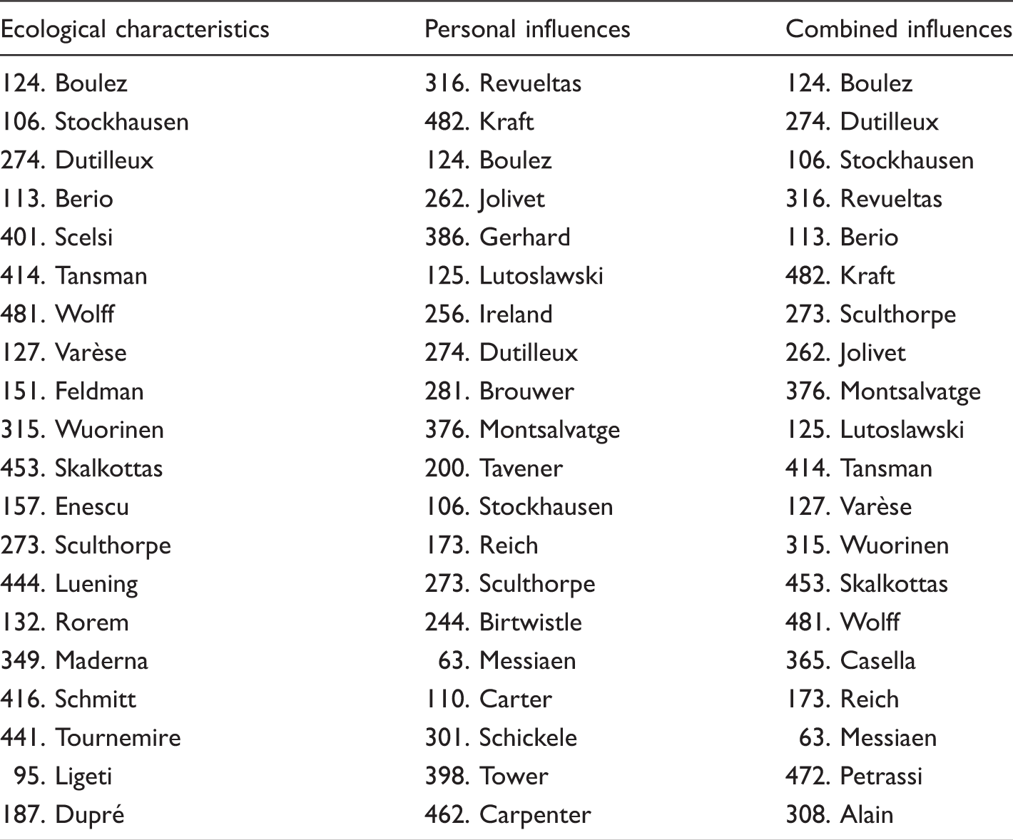
These results focus only on the relations among the major composers, however, and a more enlightening approach to overall trends can be garnered from overall rankings. First, consider Tables 4 to 6, which list the top-20 most similar composers (among all of the 500) to the top-10-ranked composers. As before, results are provided for our three different databases: Table 4 for results from common/distinct personal influences, Table 5 for results based on ecological categories, and Table 6 for results based on a combination of both personal influences and the ecological categories. Inspection of the tables reveals some considerable differences among the three. Most pointedly, there is much variation with respect to the number of names that overlap between Tables 4 and 5. For example, there are 10 names common to the two J. S. Bach lists, but only three names common to the two Chopin lists. This should not be a cause for concern, as the personal influences and ecological data sets reflect quite different kinds of information. In fact, their differences are sometimes constraining, sometimes reinforcing. The following example illustrates the constraining case.

Table 7 gives the comparative top-20 most similar listings for one individual, Iannis Xenakis, who placed number 160 in the overall CMN rankings. It will at once be noticed that, considering the avant-garde nature of Xenakis’ music, there are some rather strange names present in the first two lists (e.g., John Ireland and John Alden Carpenter in the personal influences list, and George Enescu and Charles Tournemire in the Ecological Characteristics list). These disappear, however, from the final, combined list. The latter strikes a balance taking into account both similarities of influence, and of form/period.

Table 7.

Top-20 Most Similar Composers to Iannis Xenakis, in Rank Order—All Three Similarities Data Sets (Based on Chi-square Statistics From the Binomial Index of Dispersion; Potthoff and Whittinghill, 1966).

Ecological characteristics	Personal influences	Combined influences
124. Boulez	316. Revueltas	124. Boulez
106. Stockhausen	482. Kraft	274. Dutilleux
274. Dutilleux	124. Boulez	106. Stockhausen
113. Berio	262. Jolivet	316. Revueltas
401. Scelsi	386. Gerhard	113. Berio
414. Tansman	125. Lutoslawski	482. Kraft
481. Wolff	256. Ireland	273. Sculthorpe
127. Varèse	274. Dutilleux	262. Jolivet
151. Feldman	281. Brouwer	376. Montsalvatge
315. Wuorinen	376. Montsalvatge	125. Lutoslawski
453. Skalkottas	200. Tavener	414. Tansman
157. Enescu	106. Stockhausen	127. Varèse
273. Sculthorpe	173. Reich	315. Wuorinen
444. Luening	273. Sculthorpe	453. Skalkottas
132. Rorem	244. Birtwistle	481. Wolff
349. Maderna	63. Messiaen	365. Casella
416. Schmitt	110. Carter	173. Reich
441. Tournemire	301. Schickele	63. Messiaen
95. Ligeti	398. Tower	472. Petrassi
187. Dupré	462. Carpenter	308. Alain

Table 8 gives a glimpse of the complexity of this balance. In it are listed some statistics collected from an arbitrary sample of 25 composers whose overall ranks in the CMN ranged from 1 to 240. The three statistics columns give the highest chi-squares obtained among all the matchings to each composer, for each of the three data sets. The final column indicates the number of times composers appeared among the top-40 scores for both the ecological characteristics and personal influences rankings. For example, in the case of Xenakis, the highest chi-square obtained in the ecological characteristics pairings was 92.3, the highest in the personal influences pairings 298.8, and the highest in the combined analysis pairings, 278.6. Twelve composers appeared among the top-40 contributing both to lists 1 and 2.

Table 8.

Highest Binomial Index of Dispersion Statistics (Potthoff & Whittinghill, 1966) for Each of a Sample of CMN Composers, All Three Similarities Data Sets; Number of Composers Found in Top-40 in Both (1) and (2).

CMN Rank	Composer name	Highest ecological characteristics Score (1)	Highest personal influences Score (2)	Highest combined influences Score (3)	No. of composers found in top-40 of both (1) and (2)
1.	J. S. Bach	61.5	111.6	152.1	23
10.	Chopin	68.6	156.3	133.6	8
20.	Ravel	96.8	172.1	271.1	17
30.	Gershwin	59.8	163.3	147.1	4
40.	Purcell	75.2	90.8	176.6	20
50.	Bernstein	85.1	147.9	152.2	9
60.	Scriabin	102.9	205.0	161.0	14
70.	Satie	47.7	124.2	111.8	12
80.	Palestrina	134.8	249.0	329.4	15
90.	Mascagni	259.9	131.5	376.9	8
100.	Buxtehude	121.2	103.9	170.5	15
110.	Carter	58.6	114.2	157.7	15
120.	Ginastera	49.8	158.4	128.5	9
130.	Szymanowski	54.5	200.3	157.7	10
140.	Bruch	52.0	248.0	138.5	13
150.	M. Haydn	68.9	249.5	142.0	7
160.	Xenakis	92.3	298.8	278.6	12
170.	Rubenstein	120.8	268.5	330.1	11
180.	MacDowell	148.2	318.4	296.0	12
190.	von Dohnanyi	62.4	297.6	180.6	9
200.	Tavener	57.6	185.6	118.6	4
210.	Marais	78.0	249.5	196.5	8
220.	Bridge	63.8	228.4	136.2	8
230.	Corigliano	96.0	131.5	151.1	7
240.	M. Praetorius	78.0	248.5	220.5	11

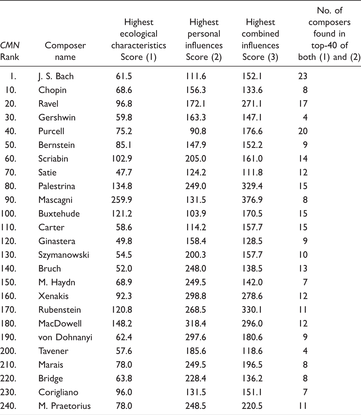
Obviously, there is a lot of variation in both the degrees of composer uniqueness, and what elements contribute to this. In Table 8, Pietro Mascagni is tightly identified by ecological characteristics including time and place, mainly his inclusion in the verismo school of opera composition (along with several other well-known composers); the result is a rather high maximum index value of 259.9. The personal influences data for Mascagni are less diagnostic, but when combined with the ecological data lead to associations with other composers that produce scores that are higher yet, maximizing at 376.9.

By contrast, the highest ecological characteristics score for Erik Satie is a rather low 47.7, and he can be regarded as a more unique individual in this sense. His highest personal influences score is also a relatively low 124.2, as is the 111.8 highest chi-square score that emerges from combining the data types. Should he perhaps be treated more on independent grounds than he usually is, when associated with Impressionist composers such as Debussy and Ravel?

In sum, there is great variation in the degrees to which each of the individual scores seem to affect the combined scores. In the Table 8 sample, Columns 1 and 3 are highly correlated (r = .814), but Columns 2 and 3 less so (r = .368, barely significant at 10% significance), suggesting a higher influence of ecological characteristics on the combined scores. Meanwhile, the means of Columns 2 and 3 are nearly the same (194.1 and 192.6), so in a considerable number of instances the highest combined score is actually lower than the highest personal influences scores alone. In some instances (e.g., Ravel, Purcell, and Palestrina), the two data sets seem to be reinforcing one another; in others (e.g., Chopin, Scriabin, and Bruch), they seem to be constraining one another. These data (and derivative sets) could lead to some interesting kinds of analysis as to the relative effects of each form of influence.

Note that the method here provides more than just a simple check against an existing general similarity assessment: The index values generated represent both a measure of the ‘distance’ between pairs of composers, and a statistical significance test. For example, as shown in Table 3, the chi-square similarity statistic for J.S. Bach and Handel is 120.96. In the dual outcome of presence/absence of common similarities and ecological categories, the degree of freedom is 1 and the critical value at a 5% significance level is thus 3.84. (For significance levels at 1% or 10%, the critical values are 6.63 and 2.70, respectively.) Because 120.96 > 3.84, we can reject the null hypothesis of no association between both composers in favor of the alternative that Bach and Handel are statistically significantly similar. For Bach and Schumann, however, the similarity index is 2.27; thus, we cannot reject the null hypothesis of no association between these two composers both at 1, 5, and 10% significance levels.

But it should also be pointed out that simple statistical significance at these levels is not by itself enough to expose obvious similarities between a given pair of composers. These data are as a set very highly ordered, and the mere sharing of as few as two influences is probably enough in most cases here to produce an association score that is statistically significant. The case of Xenakis was mentioned earlier; it turns out that both he and John Ireland (who most would agree does not have a lot in common with Xenakis in terms of actual musical product) count as influences Bartók, Debussy, and Stravinsky. Thus, much higher chi-square values should be looked to here to provide more assurance as to the existence of an ‘observable similarity’. Exactly how much higher is a debatable point for the moment, though scores of at least 50.0 for the ecological characteristics evaluations, and 100.0 for the personal influences and combined ecological characteristics/personal influences results provide reasonable ad hoc standards for now. In any case, situations such as the Xenakis/Ireland one provide food for thought: In what ways might this commonality of influence have found its way into their music in similar ways, despite returning outwardly quite different results?

Discussion and Conclusion

This paper investigates two approaches that quantify the relative similarities existing between given pairings of composers. The first approach, initially proposed by Smith and Georges (2014), infers composer similarities from the personal influences on them; the second approach applies 298 ecological categories (i.e., composer characteristics such as time period, geographical location, school association, instrumentation emphases, etc.: see Appendix) to the same ends. We originally expected the second approach to provide simple confirmation for the findings of the first, but the situation turned out to be both more complex, and more interesting, than this.

The fourth data column in Table 8 provides evidence that the two approaches produce results that are not wholly independent of one another; the column mean is 11.24, which is much greater than the value of 3.2 that would be expected were all the associations merely of random form.⁴ In that sample, there are 23 composers who are in both of the ‘top 40’ lists associated with J. S Bach, but only four who are in both for Gershwin and Tavener. Still, Bach, Gershwin, and Tavener’s ecological associations produced similar highest chi-square scores, while the ‘influences’ data produced higher highest chi-square scores for Gershwin and Tavener.

There are some fairly obvious explanations for some of the results, though these only provide glimpses. A preliminary review of all the data suggests, for example, that very high similarities scores are not restricted to either earlier or later time periods or places, though they turn up among distinct schools of composers (e.g., Italian Renaissance composers, or late 19th century ‘verismo’ opera composers). Very low scores, we might think, should be associated with composers working outside the mainstream—though many or most of these may have been too unique to generate imitators. On the other hand, some of these may have hit upon the right formula. Could it be true, in fact, that the actual most revolutionary composers are also exposed in this data set by their relatively low similarities scores? Through this line of thinking, should we consider that lasting innovation may be due more to ‘influence’ by a more unique set of personal and ecological factors than the apparent actual productions seem to indicate? J. S. Bach and Wolfgang Amadeus Mozart are two cases in point: Both of these supreme masters, neither generally thought of as being great innovators, produce rather low similarities scores (as shown in Tables 4 and 5). And, even should this kind of verdict prove attractive, perhaps this was a reality only more characteristic of earlier times than more recent ones.

It will take some time to sort through the relationships that are underscoring the results reported here, but three things appear central to such development. First, the data still suffer from some spottiness, as many of the less significant composers on the list of 500 remain incompletely studied, or even commented upon. We are hoping to reduce this problem with another large-scale literature review, currently in its planning stages.

Second, some of the ‘spottiness’ just alluded to can be reduced by adding in another set of data collected in the CMN: what might be termed general (personal) influences. These consist of influences on individual composers that are identified only generically; for example, as ‘jazz', ‘folk music', ‘Baroque composers', and so forth. Fully a third of the influences data contained in the CMN are of this type. We did not apply them at this time so as not to complicate the discussion, but once the planned literature review noted above has been completed, this information can be integrated in with the rest.

Third, it is time to start invoking some actual models that can be tested through the data, once these are satisfactorily representative. The most likely basis for such modeling is an evolutionary one—perhaps, even, a near-Darwinian one: Clearly, the overall development of Western classical music styles is not due to simple creative genius alone, but to the influence of past masters and genres, as constrained or facilitated by the cultural conditions of time and place. Darwinian biological models have been applied to many aspects of cultural evolution (see Linquist, 2010 for one good survey), but not so much to music history (but see Gatherer, 1997). While the analogy between biological change and musical change may not be a stretch, however, it remains necessary to exert some caution, as Linquist (2010) notes:

However, when conducting this sort of analysis it is important to distinguish two different sources of cultural similarity. Some shared traditions are inherited from a common ancestor while others are independently invented by a process analogous to convergent evolution. Only shared derived traditions carry information about ancestral relationships; convergent traditions are a source of noise that can generate overestimates of the relatedness among cultures. (p. xix)

Nevertheless, we believe the CMN data sets do lend themselves to a sorting out of the interplay of the relationships. In fact, the evolution of Western music may prove better represented by Darwinian thinking than do most other elements of cultural development: Not only is the time frame shorter, but so too is the spatial one, and the likelihood that, apart from the earliest stages, the ‘convergence' mentioned above may play a rather minor role in the overall process. In such work, the application of analytical models differing from the similarities approach employed here might be entertained. This would parallel trends in biological sciences systematics that have occurred over the past 50 years.

Footnotes

Declaration of Conflicting Interests

The authors declared no potential conflicts of interest with respect to the research, authorship, and/or publication of this article.

Funding

The authors received no financial support for the research, authorship, and/or publication of this article.

Notes

Author Biographies

Charles H. Smith is Science Librarian and Professor of Library Public Services at Western Kentucky University, Bowling Green, where he has worked since 1995. His Ph.D., in Geography, is from the University of Illinois; he also has advanced degrees from Indiana University and the University of Pittsburgh, and an undergraduate degree from Wesleyan University in Middletown, Connecticut. Dr. Smith has published eight books and several dozen scholarly articles, primarily on subjects in the history and philosophy of science, biogeography, systems theory, and bibliography. He is a leading student of the work of Alfred Russel Wallace. In addition to two websites on Wallace, he maintains several other ‘informational' websites and in 2013 was awarded a national lifetime President's Call to Service Award for “website development for global awareness and education”.

Patrick Georges has a Ph.D. in Economics (Ottawa, Canada), a graduate degree in International Relations and Comparative Politics (UCL-Louvain-la-Neuve, Belgium), and a degree in Applied Economics (Fucam, UCL-Mons, Belgium). He is currently an Associate Professor at the Graduate School of Public and International Affairs, University of Ottawa. Before joining the University of Ottawa in 2006, he taught at the University of British Columbia (Vancouver, Canada) and worked as a senior economist for the Canadian federal government, including for the Department of Finance and the Department of Human Resources and Skills Development. His research concerns international trade and finance, population ageing, fiscal policy and public debt management, and financial and real option pricing theory. He uses computable general equilibrium modeling, overlapping-generation computable general equilibrium modeling, and other stochastic simulation models as tools to improve understanding of the economic impacts of alternative public policies. He has also published several academic articles on classical music and classical music composers.

References

Cheetham

A. H.

Hazel

J. E.

(1969) Binary (presence-absence) similarity coefficients. Journal of Paleontology 43: 1130–1136. doi:10.2307/1302424.

Gatherer

(1997) The evolution of music – A comparison of Darwinian and dialectical methods. Journal of Social and Evolutionary Systems 20: 75–92. doi:10.1016/S1061-7361(97)90030-8.

Hayek

L.-A. C.

(1994) Analysis of amphibian biodiversity data. In: Heyer

W. R.

Donnelly

M. A.

McDiarmid

R. W.

Hayek

L.-A. C.

Foster

M. S.

(eds) Measuring and monitoring biological diversity: Standard methods for amphibians, Washington, DC: Smithsonian Books, pp. 207–269.

Jaccard

(1901) Étude comparative de la distribution florale dans une portion des Alpes et du Jura. Bull. de la Societé Vaudoise des Sciences Naturelles 37: 547–579.

Linquist

(2010) The evolution of culture, Burlington, VT: Ashgate.

Potthoff

R. F.

Whittinghill

(1966) Testing for homogeneity. I. The binomial and multinomial distributions. Biometrika 53: 167–182. doi:10.1093/biomet/53.1-2.167.

Smith

C. H.

(1983) A system of world mammal faunal regions. I. Logical and statistical derivation of the regions. Journal of Biogeography 10: 455–466.

Smith, C. H. (2000). The classical music navigator. Retrieved from http://people.wku.edu/charles.smith/music/.

Smith

C. H.

Georges

(2014) Composer similarities through “The Classical Music Navigator”: Similarity inference from composer influences. Empirical Studies of the Arts 32(2): 205–229.