






Abstract
RGB-D cameras, which give an RGB image together with depths, are becoming increasingly popular for robotic perception. In this paper, we address the task of detecting commonly found objects in the three-dimensional (3D) point cloud of indoor scenes obtained from such cameras. Our method uses a graphical model that captures various features and contextual relations, including the local visual appearance and shape cues, object co-occurrence relationships and geometric relationships. With a large number of object classes and relations, the model’s parsimony becomes important and we address that by using multiple types of edge potentials. We train the model using a maximum-margin learning approach. In our experiments concerning a total of 52 3D scenes of homes and offices (composed from about 550 views), we get a performance of 84.06% and 73.38% in labeling office and home scenes respectively for 17 object classes each. We also present a method for a robot to search for an object using the learned model and the contextual information available from the current labelings of the scene. We applied this algorithm successfully on a mobile robot for the task of finding 12 object classes in 10 different offices and achieved a precision of 97.56% with 78.43% recall.1
1. Introduction
Inexpensive RGB-D sensors that augment an RGB image with depth data have recently become widely available. These cameras are increasingly becoming the de-facto standard for perception for many robots. At the same time, years of research on SLAM (Simultaneous Localization and Mapping) has now made it possible to merge multiple RGB-D images into a single point cloud, easily providing an approximate three-dimensional (3D) model of a complete indoor scene (i.e., a room). In this paper, we explore how this move from part-of-scene two-dimensional (2D) images to full-scene 3D point clouds can improve the richness of models for object labeling.
In the past, a significant amount of work has been done in semantic labeling of 2D images (Murphy et al., 2003; Felzenszwalb et al., 2008; Heitz and Koller, 2008; Collet et al., 2011; Li et al., 2012). However, a lot of valuable information about the 3D shape and geometric layout of objects is lost when a 2D image is formed from the corresponding 3D world. A classifier that has access to a full 3D model can access important geometric properties in addition to the local shape and appearance of an object. For example, many objects occur in characteristic relative geometric configurations (e.g., a monitor is almost always on a table), and many objects consist of visually distinct parts that occur in a certain relative configuration. More generally, a 3D model makes it possible to reason about a variety of 3D properties such as 3D distances, volume and local convexity.
Some previous works have attempted to first infer the 3D structure from 2D images (Saxena et al., 2005; Hoiem et al., 2006; Divvala et al., 2009; Saxena et al., 2009) for improving object detection. However, the inferred 3D structure is not accurate enough to give significant improvement. Another recent work (Xiong and Huber, 2010) considers labeling a scene using a single 3D view (i.e., a 2.5D representation). In our work, we first use SLAM in order to compose multiple views from a Microsoft Kinect RGB-D sensor into one 3D point cloud, providing each RGB pixel with an absolute 3D location in the scene. We then (over-) segment the scene and predict semantic labels for each segment (see Figure 1). We not only predict coarse classes like in Xiong and Huber (2010) and Anguelov et al. (2005) (i.e., wall, ground, ceiling, building), but also label individual objects (e.g. printer, keyboard, monitor). Furthermore, we model rich relational information beyond an associative coupling of labels (Anguelov et al., 2005).
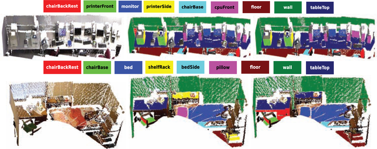
Office scene (top) and home scene (bottom) with the corresponding label coloring above the images. The left-most is the original point cloud, the middle is the ground truth labeling and the right-most is the point cloud with predicted labels.
In this paper, we propose and evaluate the first model and learning algorithm for scene understanding that exploits rich relational information derived from the full-scene 3D point cloud for object labeling and search. In particular, we propose a graphical model that naturally captures the geometric relationships of a 3D scene. Each 3D segment is associated with a node, and pairwise potentials model the relationships between segments (e.g., co-planarity, convexity, visual similarity, object co-occurrences and proximity). The model admits efficient approximate inference (Rother et al., 2007), and we show that it can be trained using a maximum-margin approach (Taskar et al., 2004; Tsochantaridis et al., 2004; Finley and Joachims, 2008) that globally minimizes an upper bound on the training loss. We model both associative and non-associative coupling of labels. With a large number of object classes, the model’s parsimony becomes important. Some features are better indicators of label similarity, while other features are better indicators of non-associative relations such as geometric arrangement (e.g., on-top-of, in-front-of). We therefore model them using appropriate clique potentials rather than using general clique potentials. Our model is thus highly flexible.
We also present an algorithm that uses the contextual information present in a 3D scene to predict where an object can be found. For example, it is more likely to find a keyboard on top of a table and in front of a monitor, and find a table drawer between the table top and the floor. A robot can use this information in many ways. The robot can move towards the contextually likely location to obtain a better view of the object, resulting in an increase in detection performance. This is especially helpful for small objects such as a keyboard that often appear as a segment with only a few points in the original view. It also helps when an object is not visible in the current view or is occluded – the robot can move to obtain additional views in contextually likely positions of the object.
We extensively evaluate our model and algorithms over a total of 52 scenes of two types: offices and homes. These scenes were built from about 550 views from the Kinect sensor. We considered the problem of labeling each segment in the scene (from a total of about 50 segments per scene) into 27 classes (17 for offices and 17 for homes, with 7 classes in common). Our experiments show that our method, which captures several local cues and contextual properties, achieves an overall performance of 84.06% on office scenes and 73.38% on home scenes.
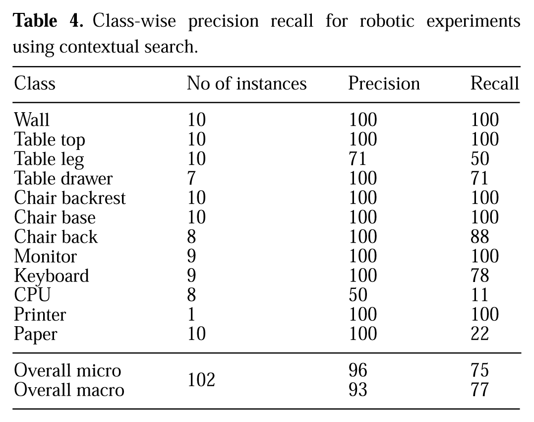
We also evaluated our labeling and contextual search algorithms on two mobile robots. In particular, in the task of finding 12 objects in 10 cluttered offices, our robot found the objects with 96% precision and 75% recall. Figure 2 shows Cornell’s Blue robot which was used in our experiments and a sample output labeling of an office scene. We have made the videos, data and the full source code (as a ROS and PCL package) available online at: http://pr.cs.cornell.edu/sceneunderstanding.

(Left) Cornell’s Blue robot mounted with an RGB-D camera (Microsoft Kinect). (Right) Predicted labeling of a scene.
2. Related Work
There is a huge body of work in the area of scene understanding and object recognition from 2D images. Previous works have focussed on several different aspects: designing good local features such as HOG (histogram-of-gradients) (Dalal and Triggs, 2005), bag of words (Csurka et al., 2004), and eigenvectors and eigenvalues of the scatter matrix (Lalonde et al., 2006), active vision for robotics (e.g., Jia et al., 2011a), and designing good global (context) features such as GIST features (Torralba, 2003). Collet et al.’s (2011) MOPED framework performs single-image and multi-image object recognition and pose estimation in complex scenes using an algorithm which iteratively estimates groups of features that are likely to belong to the same object through clustering, and then searches for object hypotheses within each of the groups.
However, the above-mentioned approaches do not consider the relative arrangement of the parts of an object or of different objects with respect to each other. It has been shown that this contextual information significantly improves the performance of image-based object detectors. A number of works propose models that explicitly capture the relations between different parts of the object, e.g., part-based models (Felzenszwalb et al., 2008), and between different objects in 2D images (Murphy et al., 2003; Heitz and Koller, 2008; Li et al., 2011). However, a lot of valuable information about the shape and geometric layout of objects is lost when a 2D image is formed from the corresponding 3D world. In some recent works, 3D layouts or depths have been used for improving object detection (e.g., Saxena et al., 2005; Hoiem et al., 2006; Leibe et al., 2007; Heitz et al., 2008; Saxena et al., 2008, 2009; Hedau et al., 2010; Lee et al., 2010; Batra and Saxena, 2012; Li et al., 2012). Here a rough 3D scene geometry (e.g., main surfaces in the scene) is inferred from a single 2D image or a stereo video stream. However, the estimated geometry is not accurate enough to give significant improvements. With 3D data, we can more precisely determine the shape, size and geometric orientation of the objects, and several other properties and therefore capture much stronger context.
Visual context can also improve the performance of object detection techniques, by providing cues about an object’s presence. Perko and Leonardis (2010) provided a method to use contextual features and train a classifier which can predict likely locations of objects, also referred to as the ‘focus of attention’, for directing object detection. In methods using active recognition, the performance of object detection for robotics is improved by letting the robots take certain actions, such as moving to an optimal location to obtain a different view of the object, based on measurements related to entropy (e.g., Denzler and Brown, 2002; Laporte et al., 2004; Laporte and Arbel, 2006; Meger et al., 2010; Ma et al., 2011). The goal here is to obtain high performance in a fewer number of actions. Jia et al. (2011b) proposes a path planning method which selects a path where the robot obtains new views of an object, and then these views are used for training the classifiers. However, these methods only use 2D images and do not have the advantage of using the rich information present in 3D data. We show that our proposed model captures context which not only helps in labeling the scene but also is able to infer most contextually likely locations of objects using the objects already found in the scene. This enables the robot to move to contextually likely locations and obtain better views for finding objects so as to improve the performance of scene labeling.
Some earlier works (Dima et al., 2004; Gould et al., 2008; Rusu et al., 2008; Quigley et al., 2009) have tried to combine shape and color information from multiple sensors for tasks such as object and obstacle detection. The recent availability of synchronized videos of both color and depth obtained from RGB-D (Kinect-style) depth cameras shifted the focus to making use of both visual as well as shape features for object detection (e.g., Lai et al., 2011a,b), 3D segmentation (e.g., Collet Romea et al., 2011), human pose estimation (e.g., Ly et al., 2012) and human activity detection (Sung et al., 2012). These methods demonstrate that augmenting visual features with 3D information can enhance object detection in cluttered, real-world environments. However, these works do not make use of the contextual relationships between various objects which have been shown to be useful for tasks such as object detection and scene understanding in 2D images. Our goal is to perform semantic labeling of indoor scenes by modeling and learning several contextual relationships.
There is also some recent work in labeling outdoor scenes obtained from Light Detection And Ranging (LIDAR) data into a few geometric classes (e.g., ground, building, trees, vegetation, etc.). Golovinskiy et al. (2009) capture context by designing node features. Xiong et al. (2011) do so by stacking layers of classifiers; however, this models only a limited correlation between the labels. An associative Markov network is used in Munoz et al. (2009), Anguelov et al. (2005) and Xiao and Quan (2009) to favor similar labels for nodes in the cliques. However, many relative features between objects are not associative in nature. For example, the relationship on-top-of does not hold in between two ground segments, i.e., a ground segment cannot be on-top-of another ground segment. Therefore, using an associative Markov network is very restrictive for our problem. Contemporary work by Shapovalov and Velizhev (2011) did address this issue by using a cutting plane method to train a non-associative Markov network. However, as we later show in our experiments, a fully non-associative Markov model is not ideal when we have a large number of classes and features. More importantly, many of the works discussed above (e.g., Anguelov et al., 2005; Munoz et al., 2009; Shapovalov et al., 2010; Shapovalov and Velizhev, 2011; Xiong et al., 2011) were designed for outdoor scenes with LIDAR data (without RGB values). Using RGB information together with depths presents some new challenges, such as designing RGB features for 3D segments. Also, since we consider a much larger number of classes compared to previous works (17 versus 3–6 for previous works), the learning task is more challenging due to the large number of parameters. We address this by proposing a parsimonious model.
The most related work to ours is that by Xiong and Huber (2010), where they label the planar patches in a point cloud of an indoor scene with four geometric labels (walls, floors, ceilings, clutter). They use a Conditional Random Field (CRF) to model geometrical relationships such as orthogonal, parallel, adjacent and coplanar. The learning method for estimating the parameters in Douillard et al. (2011) and Xiong and Huber (2010) was based on maximizing the pseudo-likelihood resulting in a sub-optimal learning algorithm. In comparison, our basic representation is 3D segments (as compared to planar patches) and we consider a much larger number of classes (beyond just the geometric classes). We also capture a much richer set of relationships between pairs of objects, and use a principled maximum-margin learning method to learn the parameters of our model.
3. Approach
We now outline our approach, including the model, its inference methods and the learning algorithm. Our input is multiple Kinect RGB-D images of a scene (i.e., a room) stitched into a single 3D point cloud using RGBDSLAM. 2 Each such combined point cloud is then over-segmented based on smoothness (i.e., difference in the local surface normals) and continuity of surfaces (i.e., distance between the points). Figure 3 shows the segmentation output for an office scene. These segments are the atomic units in our model. Our goal is to label each one of them.

(Top) Point cloud of an office scene containing two monitors and a CPU on a table and a chair beside it. (Bottom) The segmentation output of the point cloud with each segment represented with a different color. The black dots and lines represent the nodes and edges respectively of the undirected graph defined over the segments (for clarity not all nodes and edges are shown).
Before getting into the technical details of the model, we first outline the properties we aim to capture in our model:
Visual appearance. The reasonable success of object detection in 2D images shows that visual appearance is a good indicator for labeling scenes. We therefore model the local color, texture, gradients of intensities, etc., for predicting the labels. In addition, we also model the property that if nearby segments are similar in visual appearance, they are more likely to belong to the same object.
Local shape and geometry. Objects have characteristic shapes – for example, a table is horizontal, a monitor is vertical, a keyboard is uneven and a sofa is usually smoothly curved. Furthermore, parts of an object often form a convex shape. We compute 3D shape features to capture this.
Geometrical context. Many sets of objects occur in characteristic relative geometric configurations. For example, a monitor is always on-top-of a table, chairs are usually found near tables, a keyboard is in-front-of a monitor. This means that our model needs to capture non-associative relationships (e.g., that neighboring segments differ in their labels in specific patterns).
Note the examples given above are just illustrative. For any particular practical application, there will likely be other properties that could also be included. As demonstrated in the following section, our model is flexible enough to include a wide range of features.
3.1. Model formulation
We model the 3D structure of a scene using a model isomorphic to a Markov random field with log-linear node and pairwise edge potentials. Given a segmented point cloud
For a segmented point cloud
The discriminant function captures the dependencies between segment labels as defined by an undirected graph
Given
The node feature map ϕn(i) describes segment i through a vector of features, and there is one weight vector for each of the K classes. Examples of such features are the ones capturing local visual appearance, shape and geometry. The edge feature maps ϕt(i,j) describe the relationship between segments i and j. Examples of edge features are the ones capturing similarity in visual appearance and geometric context.
3
There may be multiple types t of edge feature maps ϕt(i,j), and each type has a graph over the K classes with edges Tt. If Tt contains an edge between classes l and k, then this feature map and a weight vector
We say that a type t of edge features is modeled by an associative edge potential if the corresponding graph only has self-loops, i.e.
Parsimonious model. Most of the works on 2D images have only used associative edge potentials (e.g., Szeliski et al., 2008), where the idea is that visual similarity is usually an indicator of whether two segments (or pixels) belong to same class. As discussed before, using only associative edge potentials is very restrictive for the task of object labeling and by using non-associative edge potentials we are able to model the dependencies between different objects. Examples of such dependencies are geometric arrangements such as on-top-of; we usually find a monitor, keyboard etc. on-top-of a table, rather than a table on-top-of a table. However, modeling every edge feature via a non-associative edge potential will need K2 parameters per edge feature. Therefore, the number of parameters becomes very large with an increase in the number of classes and the number of edge features. Even though, given sufficient data, a non-associative clique potential is general enough to learn associative relationships, this generality comes at an increased cost of training time and memory requirements when the number of classes is large.
We make the observation that not all features need to be modeled using non-associative edge potentials that relate every pair of classes. As described above, certain features such as the visual similarity features indicate when the two segments belong to the same class or parts of the same object, where as other geometric features capture relations between any pair of classes. A key reason for distinguishing between object-associative and non-associative features is parsimony of the model. As not all edge features are non-associative, we avoid learning weight vectors for relationships which do not exist.
Based on this observation we propose our parsimonious model (referred to as svm_mrf_parsimon) which partitions edge features into two types: object-associative features (Toa), such as visual similarity, coplanarity and convexity, which usually indicate that two segments belong to the same object, and non-associative features (Tna), such as relative geometric arrangement (e.g., on-top-of, in-front-of), which can capture characteristic configurations under which pairs of different objects occur. We model the object-associative features using object-associative potentials which capture only the dependencies between parts of the same object. The graph for this type of features contains only edges between parts of the same object and self-loops as shown in Figure 4. Formally, Toa = {(l,k)|∃object, l, k ∈ parts (object)}. The non-associative features are modeled as non-associative edge potentials. Note that |Tna| >> |Toa| since, in practice, the number of parts of an objects is much less than K. Due to this, the model we learn with both types of edge features will have much fewer numbers of parameters compared to a model learnt with all edge features as non-associative features. We show the performance of modeling the edge features using various types of edge potentials in Section 5.

Dependency graph for object-associative features. It also contains self-loops (which we do not show here for clarity).
3.2. Features
The various properties of objects and relations between them are captured in our model with the help of various features that we compute from the segmented point clouds. Our model uses two types of features: the node features and the edge features. Since,the robot knows the height and orientation of its Kinect sensor, we align all the point clouds so that the z -axis is vertical and the ground is at zero height for computing the features. Our features are insensitive to horizontal translation and rotation of the camera, but they place a lot of emphasis on the vertical direction because gravity influences the shape and relative positions of objects to a large extent. Note that, unlike images, there is no ambiguity of scale in the input point cloud and all distance measurements are in meters.
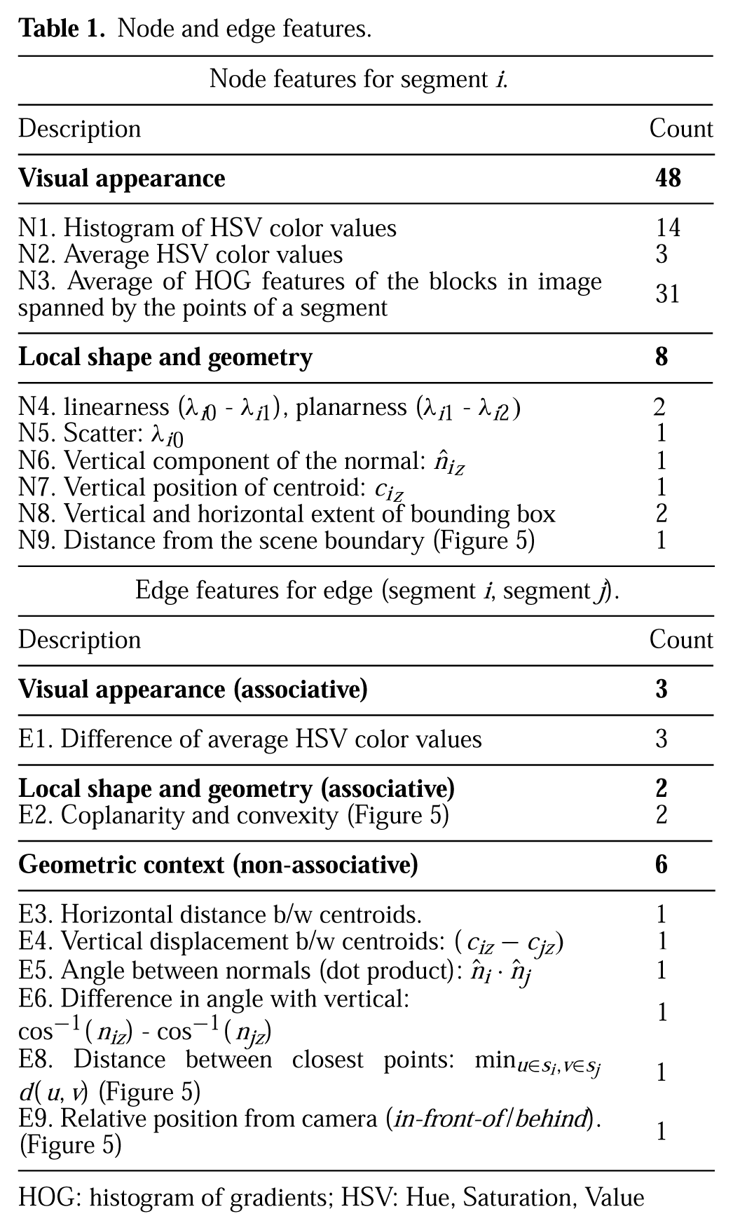
Table 1 summarizes the features used in our experiments. λi0, λi1 and λi2 are the first three eigenvalues of the scatter matrix computed from the points of segment i. si is the set of points in segment i and ci is the centroid of segment i. ri is the ray vector to the centroid of segment i from the camera position when it was captured. rhi is the projection of ri on the horizontal plane.
Node and edge features.
HOG: histogram of gradients; HSV: Hue, Saturation, Value

Illustration of a few features. (Left) Features N9 and E9. Segment i is in-front-of segment j if
The edge features ϕt(i,j) (Table 1-bottom) consist of associative features (E1–E2) based on the visual appearance and local shape, as well as non-associative features (E3–E9) that capture the tendencies of two objects to occur in certain configurations. The local shape features include coplanarity and convexity. Coplanarity is defined as
where
where dminij is the minimum distance between segments si and sj,
Finally, all the features are binned using a cumulative binning strategy. Each feature instance is represented by n binary values (each corresponding to a bin), where n is the number of bins. n thresholds are computed where the ith one is the
3.3. Computing predictions
Our goal is to label each segment in the segmented point cloud with the most appropriate semantic label. This is achieved by finding the label assignment which maximizes the value of the discriminant function in equation (2). Given the learned parameters of the model and the features computed from the segmented point cloud, we need to solve the argmax in equation (1) for the discriminant function in equation (2). This is NP hard. It can be equivalently formulated as the following mixed-integer program.
Note that the products
However, when using our algorithm on labeling new scenes (e.g., during our robotic experiments), objects other than the 27 objects we modeled might be present. Forcing the model to predict one of the 27 objects for all segments would result in wrong predictions for every segment of an unseen class. Therefore, we relax the constraints
We further relax the problem by removing the constraints in equation (5) and let the variables
The relaxation solution
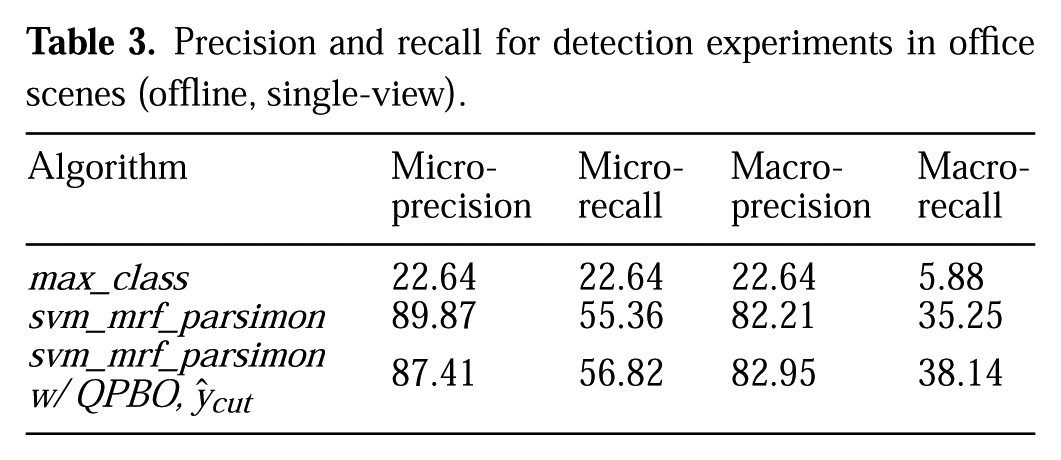
In Section 5, Table 3 shows that the solution
3.4. Learning algorithm
We take a large-margin approach to learning the parameter vector
Our method optimizes a regularized upper bound on the training error
where
While the number of constraints in this quadratic program is exponential in n, N and K, it can nevertheless be solved efficiently using the cutting-plane algorithm for training structural Support Vector Machines (SVMs) (Joachims et al., 2009). The algorithm maintains a working set of constraints, and it can be shown to provide an ε -accurate solution after adding at most O(R2C/ε) constraints (ignoring log terms). The algorithm merely needs access to an efficient method for computing
Due to the structure of Δ(.,.), this problem is identical to the relaxed prediction problem in equations (3) and (4) and can be solved efficiently using graph cuts.
Since our training problem is an overgenerating formulation as defined in Finley and Joachims (2008), the value of
4. Contextual search
In robotic tasks such as that of finding objects, a robot might not find the object it was looking for in its current view. The object might be far away, occluded or even out of view. In this section, we propose a method which determines the optimal location for the robot to move to for finding the object it was looking for. Our method uses the context from the objects already identified in the robot’s current view.
Formally, the goal is to find the 3D location where the desired object is most likely to be found, given a (partially) labeled point cloud. This can be done by sampling 3D locations in the current view and using the learned discriminant function to compare the chances of finding the desired object at those locations. We generate these samples by discretizing the 3D bounding box of the labeled point cloud and considering the centre of each grid as a sample. We considered 1000 equally spaced samples in our experiments.
4.1. Augmented graph
To evaluate the score of a sample (lx, ly, lz) we first generate a graph on which the discriminant function can be applied. For this, we first take the graph of labeled segments (labeled using our algorithm) and augment it with a node h corresponding to a hallucinated segment xh at location (lx, ly, lz). We then add edges between this node, h, and the nearby nodes (labeled segments) that are within context_ range distance from the sampled location. We denote these neighboring segments of the hallucinated segment by Nbr(xh). Suppose we are looking for an (missing) object class k, we label the newly added node as class k, i.e., the k th element of yh is 1 and the rest are 0. Figure 6 illustrates one such augmentation step. We can now apply our discriminant function to this augmented graph. Note that each of our sampled locations will give us a unique corresponding augmented graph.
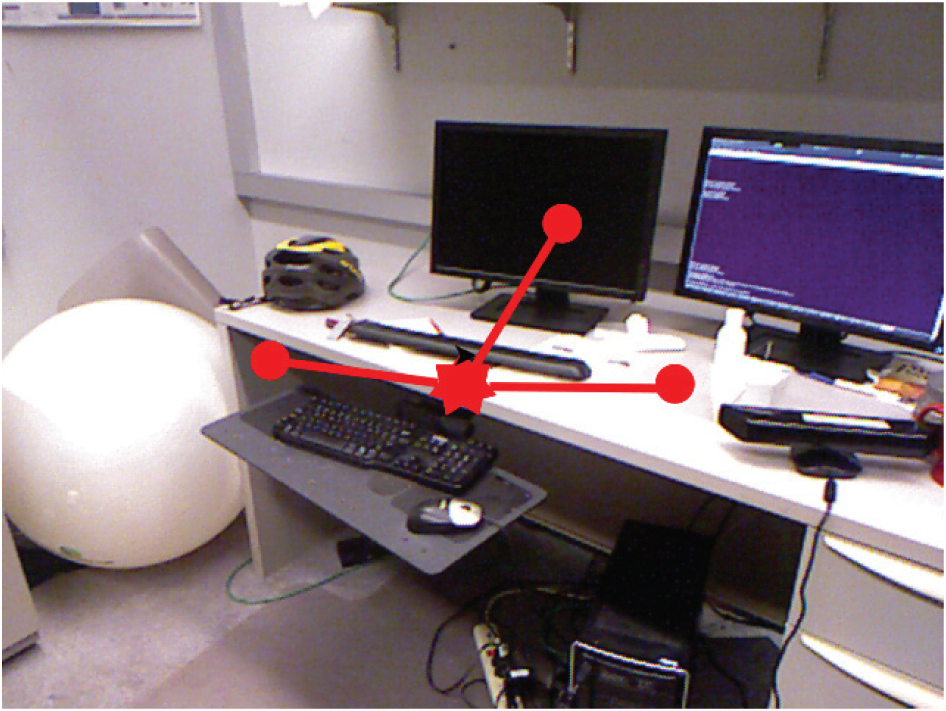
Figure illustrating our method for contextual search. The location of the hallucinated segment is shown by a red star and its neighbors are denoted using red edges. In this particular scene the hallucinated keyboard segment is connected to the monitor, table-top and table-leg segments. The keyboard and tray segments were left unlabeled by the algorithm, so they are not connected.
4.2. Discriminant function and inference
We use the discriminant function from equation (2) to compute the score of each augmented graph. The optimal sample (location) for finding an instance of class k, OL(k), is the one with highest value of the discriminant function applied to its corresponding augmented graph. Note that only the location-dependent terms in the discriminant function for the newly added node and edges can effect its value, since the rest of the terms are the same for every sample. Thus, we can compute OL(k) very efficiently.
We denote the sum of all terms of the discriminant function which do not depend on the location (lx, ly, lz) by a constant ρ. We denote the label of a node j in the original labeled graph (before augmentation) as label(j). Let ϕ′ n (h) denote the features of the hallucinated node h, which only depend on its location (lx, ly, lz). Similarly, let ϕt′(h, j) denote the features of the edge (h, j) which only depend on the location of the hallucinated node. Let w′ n and w′ t denote the projection of node and edge weight vectors respectively that contain only the components corresponding to the location-dependent features. Now we can formally define the optimal location as
where
Once the optimal location OL(k) is found by solving equation (9), the robot moves close to this location to find objects as described in our contextually guided object detection experiments presented in Section 5.5.
5. Experiments
In this section, we first describe our dataset and present results of the scene labeling task on this dataset. We present a detailed analysis of various factors such as the effect of the 3D features, the effect of adding context, the effect of the presence of unlabeled segments, etc.
We then present the results on robotic experiments on attribute learning and contextually guided object detection. The object detection experiments were performed using two robots: Cornell’s Blue and POLAR robots, as shown in Figure 7 and Figure 8 respectively. These robots consist of a mobile base (Erratic and Segway Omni 50 respectively) and were mounted with Kinect sensors as shown in the respective figures. (For more details on the hardware specification of the POLAR robot, please see Jiang et al., 2012.) We used ROS libraries 6 to program these robots.
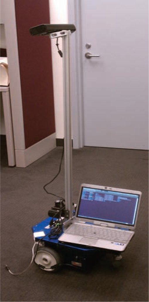
Cornell’s Blue robot. It consists of a mobile base mounted with a Kinect sensor.
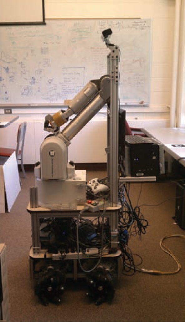
Cornell’s POLAR (PersOnaL Assistant Robot) robot. It consists of a omni-directional mobile base with a robotic arm and Kinect sensor mounted on the top.
5.1. Data
We consider labeling object segments in full 3D scenes (as compared to 2.5D data from a single view). For this purpose, we collected data of 24 office and 28 home scenes from a total of about 550 views. Each scene was reconstructed from about 8–9 RGB-D views from a Microsoft Kinect sensor and contains about one million colored points. We first over-segment the 3D scene (as described earlier) to obtain the atomic units of our representation. For training, we manually labeled the segments, and we selected the labels which were present in a minimum of five scenes in the dataset. Specifically, the office labels are {wall, floor, tableTop, tableDrawer, tableLeg, chairBackRest, chairBase, chairBack, monitor, printerFront, printerSide keyboard, cpuTop, cpuFront, cpuSide, book, paper}, and the home labels are {wall, floor, tableTop, tableDrawer, tableLeg, chairBackRest, chairBase, sofaBase, sofaArm, sofaBackRest, bed, bedSide, quilt, pillow, shelfRack, laptop, book}. This gave us a total of 1108 labeled segments in the office scenes and 1387 segments in the home scenes. Often one object may be divided into multiple segments because of over-segmentation. We have made this data available at http://pr.cs.cornell.edu/sceneunderstanding/data/data.php.
5.2. Segmentation
For segmenting the point cloud, we use a region growing algorithm similar to the Euclidean clustering in the Point-Cloud Library (PCL). 7 It randomly picks a seed point and grows it into a segment. New points are added to an existing segment if their distance to the closest point in the segment is less than a threshold and the local normals calculated at these points are at an angle less than a threshold. We also made the distance threshold proportional to the distance from the camera because points far from the camera have more noisy depth estimates. In detail, we used a distance threshold of 0.1d, where d is the distance of the candidate point from the camera, and an angle threshold of 30∘. We observed that these thresholds slightly over-segmented almost all scenes into object-parts of desired granularity. Such a simple approach would not perfectly segment all objects, but we find that our learning method is quite robust to such noisy segmentation.
5.3. Object labeling results
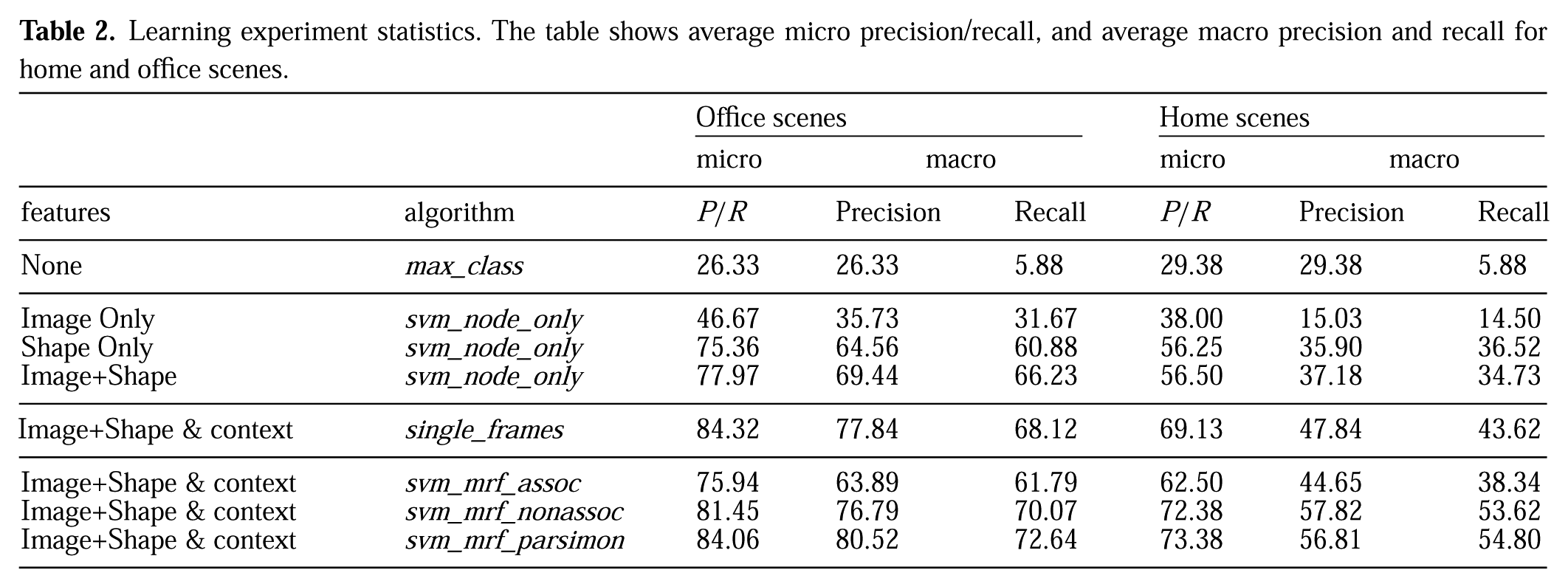
In this subsection, we report the results of offline labeling experiments. Table 2 shows the results, performed using four-fold cross-validation and averaging performance across the folds for the models trained separately on the home and office datasets. We use both macro and micro averaging to aggregate precision and recall over various classes.
Learning experiment statistics. The table shows average micro precision/recall, and average macro precision and recall for home and office scenes.
Let predi(k) denote that the ith segment was predicted to be of class k, and gti(k) denote that the ground truth label of the ith segment was class k. We now formally define the following metrics used in the literature.
where, for any set S, |S| denotes its size.
In these experiments, prediction is done using an MIP solver with the constraint that a segment can have exactly one label (
Figure 1 shows the original point cloud, ground-truth and predicted labels for one office (top) and one home scene (bottom). Figure 9 shows the confusion matrices for office and home scenes on the left and right respectively. For the majority of the classes our model predicts the correct label as can be seen from the strong diagonal in the confusion matrices. Some of the mistakes are reasonable, such as a pillow getting confused with the quilt in homes. They often have similar location and texture. In offices, books placed on table-tops sometimes get confused with the table-top.
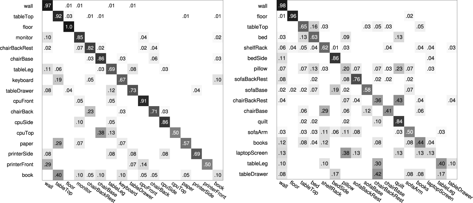
Confusion matrix on the office dataset (left) and home dataset (right) with svm_mrf_parsimon trained on Shape and Image features.
One of our goals was to study the effect of various factors, and therefore we compared our algorithm with various settings. We discuss them in the following.
The type of contextual relations we capture depend on the type of edge potentials we model. To study this, we compared our method with models using only associative or only non-associative edge potentials referred to as svm_mrf_assoc and svm_mrf_nonassoc. We observed that modeling all edge features using associative potentials is poor compared to our full model. In fact, using only associative potentials showed a drop in performance compared to svm_node_only model on the office dataset. This indicates it is important to capture the relations between regions having different labels. Our svm_mrf_nonassoc model does so by modeling all edge features using non-associative potentials, which can favor or disfavor labels of different classes for nearby segments. It gives higher precision and recall compared to svm_node_only and svm_mrf_assoc. This shows that modeling using non-associative potentials is a better choice for our labeling problem.
However, not all the edge features are non-associative in nature, modeling them using only non-associative potentials could be an overkill (each non-associative feature adds K2 more parameters to be learnt). Therefore using our svm_mrf_parsimon model to model these relations achieves higher performance in both datasets.
In order to study this, we compared our svm_mrf_parsimon with varying context_ range for determining the neighborhood (see Figure 10 for a plot of average micro precision versus range). Note that the context_ range is determined from the boundary of one segment to the boundary of the other, and hence it is somewhat independent of the size of the object. We note that increasing the context_ range increases the performance to some level, and then it drops slightly. We attribute this to the fact that with increasing the context_ range, irrelevant objects may get an edge in the graph, and with limited training data, spurious relationships may be learned. We observe that the optimal context_ range for office scenes is around 0.3 m and that for homes scenes is 0.6 m.
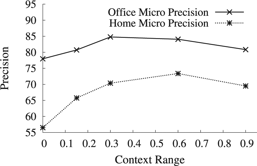
Effect of context range on precision (= recall here).
What is the effect of the inference method? The results for the svm_mrf algorithms in Table 2 were generated using the MIP solver. The QPBO algorithm however, gives a higher precision and lower recall on both datasets. For example, on office data, the graph cut inference for our svm_mrf_parsimon algorithm gave a micro precision of 90.25% and a micro recall of 61.74%. Here, the micro precision and recall are not the same as some of the segments might not get any labels.
5.4. Attribute labeling results
In some robotic tasks, such as robotic grasping, it is not necessary to know the exact object category, but just knowing a few attributes of an object may be useful. For example, if a robot has to clean a floor, it would help if it knows which objects it can move and which it cannot. If it has to place an object, it should place them on horizontal surfaces, preferably where humans do not sit. With this motivation we have designed eight attributes, each for the home and office scenes, giving a total of 10 unique attributes. They are {wall, floor, flat-horizontal-surfaces, furniture, fabric, heavy, seating-areas, small-objects, table-top-objects, electronics}. Note that each segment in the point cloud can have multiple attributes and therefore we can learn these attributes using our model which naturally allows multiple labels per segment. We compute the precision and recall over the attributes by counting how many attributes were correctly inferred. In home scenes we obtained a precision of 83.12% and 70.03% recall, and in the office scenes we obtained 87.92% precision and 71.93% recall.
5.5. Robotic experiments
The ability to label scenes is very useful for robotics applications, such as for finding/retrieving an object on request. As described in Section 3.3, in a detection scenario there can be some segments not belonging to the object classes we consider. Table 3 shows the results of running our inference algorithms for detection scenarios on the offline office dataset when considering all segments, including those belonging to classes other than the 17 mentioned earlier. The solution of the relaxed MIP (described in Section 3.3) gives us high precision (89.87% for micro, and 82.21% for macro), but low recall (55.36% for micro, and 35.25% for macro). The
Precision and recall for detection experiments in office scenes (offline, single-view).
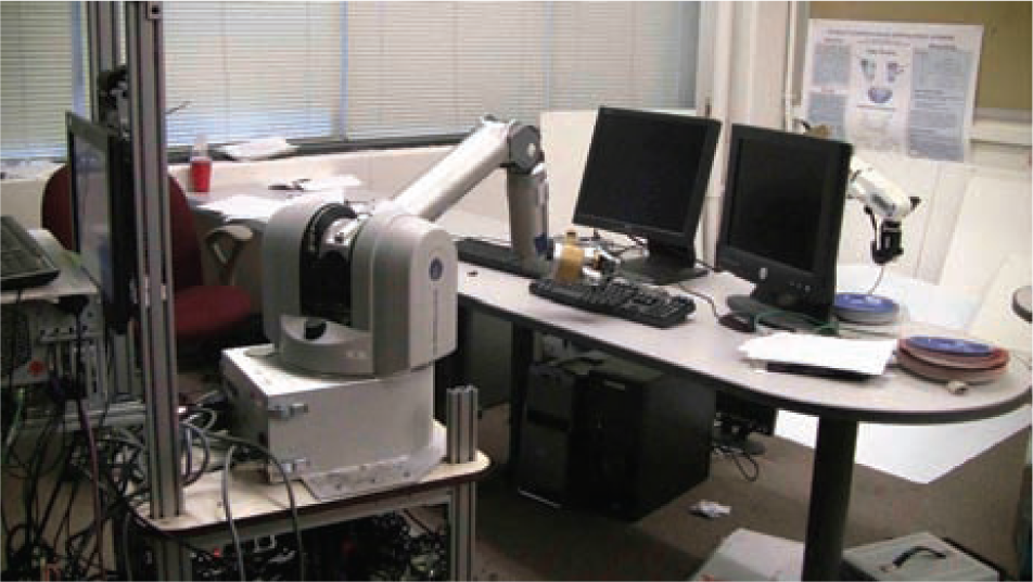
Cornell’s POLAR robot using our classifier for detecting a keyboard in a cluttered room.
In order to evaluate our contextual search algorithm, we test our approach on our Blue robot for the task of finding 12 object classes located in 10 office scenes. The robot starts from a pre-determined location in an office and searches for a given list of objects in the room. The goal of the robot is to find at least one instance for each of the object classes it is asked to search for. Since, the RGB-D sensor has a narrow field-of-view (57 degrees horizontally), the robot first scans the room by turning a fixed angle each time. It labels the point cloud it obtains in each view and saves the labeled point clouds.
Next, for all the object classes it did not find, it computes the contextually likely locations for the objects using the algorithm described in Section 4. Using the inferred locations, the robot moves in that direction in order to get a better view of the objects. Figure 12 shows the experiment run in one office scene. The first column shows the Blue robot and the scene in which it is asked to find the objects and the rest of the columns show the sequence of colored images corresponding to the labeled point clouds. The first two point clouds were obtained when the robot was scanning the room from a distance, and the last two are obtained after inferring the contextually likely locations of the objects not found and moving closer to these locations. Table 4 shows the precision and recall of finding the 12 object classes in our robotic experiments.
Class-wise precision recall for robotic experiments using contextual search.

(Left): The robot in an office scene. (Columns 2–5): sequence of colored images corresponding to the labeled point clouds generated by the robot during the object detection experiment.
To evaluate our contextual search algorithm, we present both qualitative and quantitative results. Figure 13 qualitatively shows the predictions for finding monitor, keyboard, table drawer and paper in a frame in which they were not found. These heatmaps are generated in 3D, but for visualization purposes they are aligned to the original RGB image in Figure 13. As can be seen form Figure 13, a monitor is predicted to be most likely found above the table and a table drawer is likely to be found under the table top. However, it does not do a great job for paper, and this may be because we had very few examples for this class in our training set.
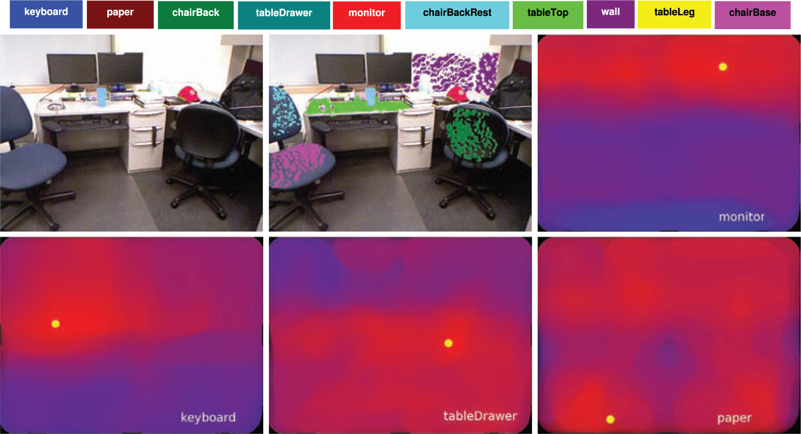
(Top left) Original image. (Top mid) Inferred labels color-coded using the legend shown above. (Top right, bottom left, bottom mid and bottom right) Contextually likely positions for finding monitor, keyboard, table drawer and paper, respectively. In these heatmaps, red indicates that the target object is more likely to be found there. The circular yellow dot indicates the most likely location.
Figure 14 shows that our algorithm can also be used on a robot to find objects even when they are occluded. Clearly, it predicts that a keyboard is likely to be found in front of the monitor and at about the same height as the table top. To quantitatively evaluate the predictions, we collected 10 frames where a keyboard was not detected, but other objects such as table and monitor were detected. We then applied our contextual search algorithm to find the optimal 3D locations for finding a keyboard. For each of these scenes, we computed the minimum distance of the actual keyboard points to the inferred optimal location. As a baseline, if the predictor always predicted midpoints of the scene as the probable location of the keyboard, the max, mean and median values over 10 scenes were 113.5 cm, 32.6 cm and 27.2 cm respectively. Using our method, we get 36.3 cm, 17.5 cm and 15.9 cm respectively. We found that this helps the robot in finding the objects with only a few moves.
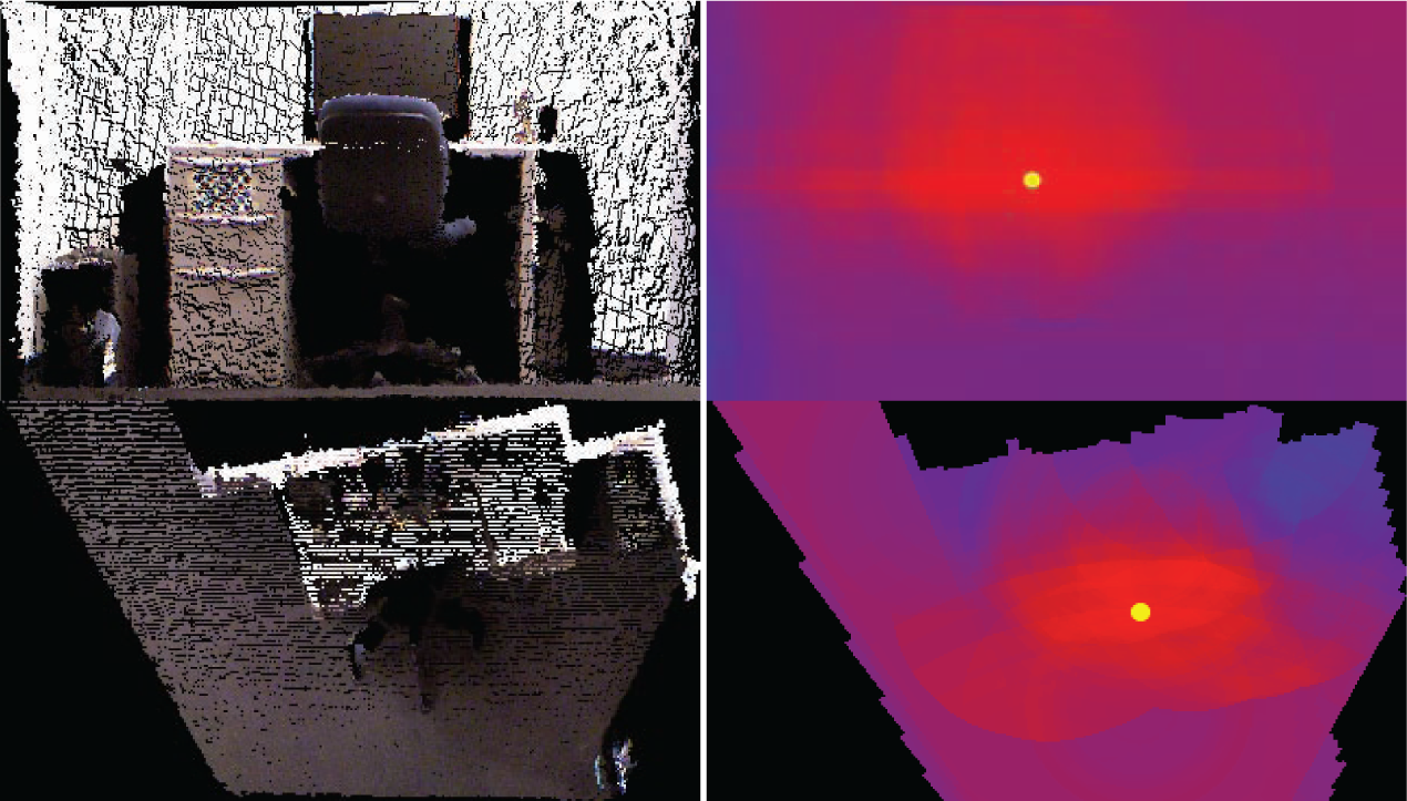
(Left column) Front and top views (orthographic projections) of an office scene in which a keyboard is occluded. (Right column) Corresponding heatmaps where red indicates that the keyboard is more likely to be found there. The yellow dot indicates the most likely location.
We have the code available as a ROS and PCL package. Code, datasets as well as videos showing our robots finding objects using our algorithm are available at http://pr.cs.cornell.edu/sceneunderstanding/.
6. Conclusion
In conclusion, we have proposed and evaluated the first model and learning algorithm for semantic labeling that exploits rich relational information in full-scene 3D point clouds. Our method captures various features and contextual relations, including the local visual appearance and shape cues, object co-occurrence relationships and geometric relationships. We have shown how visual and shape features can be modeled parsimoniously when the number of classes is large. We have also presented an algorithm to infer contextually likely locations for the desired objects given the current labelings in the scene. We tested our method on a large offline dataset, as well as on the task of mobile robots finding objects in cluttered scenes.
Footnotes
Acknowledgements
We thank Gaurab Basu, Yun Jiang, Jason Yosinski and Dave Kotfis for help with the robotic experiments.
Notes
Funding
This research was funded in part by a Microsoft Faculty Fellowship and Alfred P. Sloan Research Fellowship to one of us (Saxena), and by NSF Award IIS-0713483.