Variable risk control via stochastic optimization

Abstract

We present new global and local policy search algorithms suitable for problems with policy-dependent cost variance (or risk), a property present in many robot control tasks. These algorithms exploit new techniques in non-parametric heteroscedastic regression to directly model the policy-dependent distribution of cost. For local search, the learned cost model can be used as a critic for performing risk-sensitive gradient descent. Alternatively, decision-theoretic criteria can be applied to globally select policies to balance exploration and exploitation in a principled way, or to perform greedy minimization with respect to various risk-sensitive criteria. This separation of learning and policy selection permits variable risk control, where risk-sensitivity can be flexibly adjusted and appropriate policies can be selected at runtime without relearning. We describe experiments in dynamic stabilization and manipulation with a mobile manipulator that demonstrate learning of flexible, risk-sensitive policies in very few trials.

Keywords

policy search Bayesian optimization robot learning risk-sensitive dynamic mobile manipulation

1. Introduction

Experiments on physical robot systems are typically associated with significant practical costs, such as experimenter time, money, and robot wear and tear. However, such experiments are often necessary to refine controllers that have been hand designed or optimized in simulation. This necessity is a result of the extreme difficulty associated with constructing model systems of sufficiently high fidelity that behaviors translate to hardware without performance loss. For many nonlinear systems, it can even be infeasible to perform simulations or construct a reasonable model (Roberts et al., 2010).

For this reason, model-free policy search methods have become one of the standard tools for constructing controllers for robot systems (Rosenstein and Barto, 2001; Kohl and Stone, 2004; Tedrake et al., 2004; Peters and Schaal, 2006; Lizotte et al., 2007; Kober and Peters, 2009; Kolter and Ng, 2010; Theodorou et al., 2010). These algorithms are designed to minimize the expected value of a noisy cost signal, $\hat{J} (θ)$ , by adjusting policy parameters, θ , for a fixed class of policies, u = π_θ(x, t). By considering only the expected cost of a policy and ignoring cost variance, the solutions found by these algorithms are by definition risk-neutral, where risk corresponds to a monotonic function of the cost variance. However, for systems that operate in a variety of contexts, it can be advantageous to have a more flexible attitude toward risk.

For example, imagine a humanoid robot that is capable of several dynamic walking gaits that differ based on their efficiency, speed, and predictability. When operating near a large crater, it might be reasonable to select a more predictable, possibly less energy-efficient gait over a less predictable, higher performance gait. Likewise, when far from a power source with low battery charge, it may be necessary to risk a fast and less predictable policy because alternative gaits have comparatively low probability of achieving the required speed or efficiency. To create flexible systems of this kind, it will be necessary to design optimization processes that produce control policies that differ based on their risk.

Recently there has been increased interest in applying Bayesian optimization algorithms to solve model-free policy search problems (Lizotte et al., 2007; Martinez-Cantin et al., 2007, 2009; Kuindersma et al., 2011; Tesch et al., 2011; Wilson et al., 2011). In contrast to well-studied policy gradient methods (Peters and Schaal, 2006), Bayesian optimization algorithms perform policy search by modeling the distribution of cost in policy parameter space and applying a selection criterion to globally select the next policy. Selection criteria are typically designed to balance exploration and exploitation with the intention of minimizing the total number of policy evaluations. These properties make Bayesian optimization attractive for robotics since cost functions often have multiple local minima and policy evaluations are typically expensive. It is also straightforward to incorporate approximate prior knowledge about the distribution of cost (such as could be obtained from simulation) and enforce hard constraints on the policy parameters.

Previous implementations of Bayesian optimization have assumed that the variance of the cost is the same for all policies in the search space. This is not true in general. In this work, we propose a new type of Bayesian optimization algorithm that relaxes this assumption and efficiently captures both the expected cost and cost variance during the optimization. Specifically, we extend recent work developing a variational Gaussian process (GP) model for problems with input-dependent noise (or heteroscedasticity) (Lázaro-Gredilla and Titsias, 2011) to the optimization case by deriving an expression for expected improvement (EI) (Močckus et al., 1978), a commonly used criterion for selecting the next policy, and incorporating log priors into the optimization to improve numerical performance. We also consider the use of confidence bounds (CBs) to produce runtime changes to risk-sensitivity and derive a generalized expected risk improvement (ERI) criterion that balances exploration and exploitation in risk-sensitive setting. Finally, we consider a simple local search procedure that uses the learned cost model as a critic for performing risk-sensitive stochastic gradient descent (RSSGD). We evaluate these algorithms in dynamic stabilization and manipulation experiments with the uBot-5 mobile manipulator.

2. Background

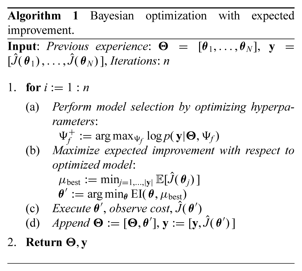
2.1. Bayesian optimization

Bayesian optimization algorithms are a family of global optimization techniques that are well suited to problems where noisy samples of an objective function are expensive to obtain (Lizotte et al., 2007; Frean and Boyle, 2008; Brochu et al., 2009; Martinez-Cantin et al., 2009; Tesch et al., 2011; Wilson et al., 2011). In describing these algorithms, we use the language of policy search where the inputs are policy parameters and outputs are costs. However, these algorithms are applicable to general stochastic nonlinear optimization problems not related to control (Brochu et al., 2009).

2.1.1. GPs

Most Bayesian optimization implementations represent the prior over cost functions as a GP. A GP is defined as a (possibly infinite) set of random variables, any finite subset of which is jointly Gaussian distributed (Rasmussen and Williams, 2006). In our case the random variable is the cost, $\hat{J} (θ)$ , which is indexed by the set of policy parameters. The GP prior, $J (θ) ~ G P (m (θ), k_{f} (θ, θ^{'}))$ , is fully specified by its mean function and covariance (or kernel) function,

\begin{array}{l} m (θ) & = & E [J (θ)], \\ k_{f} (θ, θ^{'}) & = & E [(J (θ) - m (θ^{'})) (J (θ) - m (θ^{'}))] . \end{array}

Typically, we set m( θ ) = 0 and let k_f( θ , θ ^′) take on one of several standard forms. A common choice is the anisotropic squared exponential kernel,

k_{f} (θ, θ^{'}) = σ_{f}^{2} exp (- \frac{1}{2} {(θ - θ^{'})}^{⊤} M (θ - θ^{'})),

(1)

where $σ_{f}^{2}$ is the signal variance and $M = diag (ℓ_{f}^{- 2})$ is a diagonal matrix of length-scale hyperparameters. Intuitively, the signal variance hyperparameter captures the overall magnitude of the cost function variation and the length-scales capture the sensitivity of the cost with respect to changes in each policy parameter. The squared exponential kernel is stationary since it is a function of θ − θ ^′, i.e. it is invariant to translations in parameter space. In some applications, the target function will be non-stationary: flat in some regions, with large changes in others. There are kernel functions appropriate for this case (Rasmussen and Williams, 2006), but in this work we use the squared exponential kernel (1) exclusively.

Samples of the unknown cost function are typically assumed to have additive independent and identically distributed (i.i.d.) noise,

\hat{J} (θ) = J (θ) + ε, ε ~ N (0, σ_{n}^{2}) .

(2)

Given the GP prior and data,

\begin{array}{l} Θ & = & {[θ_{1}, θ_{2}, \dots, θ_{N}]}^{⊤} \in ℝ^{N \times dim (θ)}, \\ y & = & {[\hat{J} (θ_{1}), \hat{J} (θ_{2}), \dots, \hat{J} (θ_{N})]}^{⊤} \in ℝ^{N}, \end{array}

the posterior (predictive), cost distribution can be computed for a policy parameterized by θ _* as, ${\hat{J}}_{*} \equiv \hat{J} (θ_{*}) ~ N (E [{\hat{J}}_{*}], s_{*}^{2})$ ,

\begin{array}{l} E [{\hat{J}}_{*}] & = & k_{f *}^{⊤} {(K_{f} + σ_{n}^{2} I)}^{- 1} y, \\ s_{*}^{2} & = & k_{f} (θ_{*}, θ_{*}) - k_{f *}^{⊤} {(K_{f} + σ_{n}^{2} I)}^{- 1} k_{f *}, \end{array}

where k_f* = [k_f( θ ₁, θ _*), k_f( θ ₂, θ _*),…, k_f( θ _N, θ _*)]^⊤ and K_f is the positive-definite kernel matrix, [K_f]_ij = k_f( θ _i, θ _j).

If prior information regarding the shape of the cost distribution is available, e.g., from simulation experiments, the mean function and kernel hyperparameters can be set accordingly (Lizotte et al., 2007). However, in many cases such information is not available and model selection must be performed. Typically, when the hyperparameters, Ψ_f = {σ_f, ℓ _f, σ_n}, are unknown, the log marginal likelihood, log p(y|Θ, Ψ_f), is used to optimize their values before computing the posterior (Rasmussen and Williams, 2006). The log marginal likelihood and its derivatives can be computed in closed form, so we are free to choose from standard nonlinear optimization methods to maximize the marginal log likelihood for model selection.

2.1.2. Expected improvement

To select the (N + 1) th policy parameters, an offline optimization of a selection criterion is performed with respect to the posterior cost distribution. A commonly used criterion is EI (Močkus et al., 1978; Brochu et al., 2009). Expected improvement is defined as the expected reduction in cost, or improvement, over the best policy previously evaluated. The improvement of a policy parameter θ _* is defined as

I_{*} = {\begin{matrix} μ_{best} - {\hat{J}}_{*} & if {\hat{J}}_{*} < μ_{best}, \\ 0 & otherwise, \end{matrix}

(3)

where $μ_{best} = {min}_{i = 1, \dots, N} E [\hat{J} (θ_{i})]$ . Since the predictive distribution under the GP model is Gaussian, the expected value of I_* is

\begin{array}{l} EI (θ_{*}) & = & \int_{0}^{\infty} I_{*} p (I_{*}) d I_{*}, \\ = & s_{*} (u_{*} Φ (u_{*}) + φ (u_{*})) \end{array}

(4)

where $u_{*} = (μ_{best} - E [{\hat{J}}_{*}]) / s_{*}$ , and Φ(⋅) and ɸ(⋅) are the cumulative distribution function (CDF) and probability density function (PDF) of the normal distribution, respectively. If s_* = 0, the EI is defined to be 0. Both (4) and its gradient, ∂EI ( θ ) / ∂ θ , are efficiently computable, so we can apply standard nonlinear optimization methods to maximize EI to select the next policy. In practice, a parameter ξ is often used to adjust the balance of exploration and exploitation, $u_{*} = (μ_{best} - E [{\hat{J}}_{*}] + ξ) / s_{*}$ , where ξ > 0 leads to an optimistic estimate of improvement and tends to encourage exploration. Setting ξ > 0 can be interpreted as increasing the expected cost of θ _best by ξ. Lizotte et al. (2011) showed that cost scale invariance can be achieved by multiplying ξ by the signal standard deviation, σ_f. The Bayesian optimization with EI algorithm is shown in Algorithm 1.

Algorithm 1 Bayesian optimization with expected improvement.
Input: Previous experience: $Θ = [θ_{1}, \dots, θ_{N}], y = [\hat{J} (θ_{1}), \dots, \hat{J} (θ_{N})]$ , Iterations: n
1. for i:= 1: n
(a) Perform model selection by optimizing hyperparameters:
$Ψ_{f}^{+} : = arg {max}_{Ψ_{f}} log p (y \| Θ, Ψ_{f})$
(b) Maximize expected improvement with respect to optimized model:
$μ_{best} : = {min}_{j = 1, \dots, \| y \|} E [\hat{J} (θ_{j})]$
θ ^′:= arg min_θEI ( θ , μ_best)
(c) Execute θ ^′, observe cost, $\hat{J} (θ^{'})$
(d) Append Θ:= [Θ, θ ^′], $y : = [y, \hat{J} (θ^{'})]$
2. Return Θ, y

From a theoretical perspective, Vazquez and Bect (2010) proved that using EI selection for Bayesian optimization converges for all cost functions in the reproducing kernel Hilbert space of the GP covariance function and almost surely for all functions drawn from the GP prior. However, these results rest on the assumption that the GP hyperparameters remain fixed throughout the optimization. Recently, Bull (2011) proved convergence rates for EI selection with fixed hyperparameters and the case where model selection is performed according to a modified maximum marginal likelihood procedure. The general case of applying Bayesian optimization with maximum marginal likelihood model selection and EI policy selection is not guaranteed to converge to the global optimum.

Although EI is a commonly used selection criterion, a variety of other criteria have been studied. For example, early work by Kushner (1964) considered the probability of improvement as a criterion for selecting the next input. CB criteria (discussed in Section 3.2) have been extensively studied in the context of global optimization (Cox and John, 1992; Srinivas et al., 2010) and economic decision making (Levy and Markowitz, 1979). Recent work (Osborne et al., 2009; Garnett et al., 2010) has considered multi-step lookahead criteria that are less myopic than methods that only consider the next best input. For an excellent tutorial on Bayesian optimization, see Brochu et al. (2009).

2.2. Variational heteroscedastic Gaussian process regression

One limitation of the standard regression model (2) is the assumption of i.i.d. noise over the input space. Many data do not adhere to this simplification and models capable of capturing input-dependent noise (or heteroscedasticity) are required. The heteroscedastic regression model takes the form

\hat{J} (θ) = J (θ) + ε_{θ}, ε_{θ} ~ N (0, r {(θ)}^{2}),

(5)

where the noise variance, r( θ )², is dependent on the input, θ . In the Bayesian non-parametric setting, a second GP prior,

g (θ) ~ G P (μ_{0}, k_{g} (θ, θ^{'})),

is placed over the unknown log variance function, g( θ ) ≡logr( θ )² (Goldberg et al., 1998; Kersting et al., 2010; Lázaro-Gredilla and Titsias, 2011).¹ This prior, when combined with the cost prior (Section 2.1.1), forms the heteroscedastic Gaussian process (HGP) model. Unfortunately, the HGP model has the property that the computations of the posterior distribution and the marginal log likelihood are intractable, thus making model selection and prediction difficult.

Stochastic techniques, such as Markov chain Monte Carlo (MCMC) (Goldberg et al., 1998), offer a principled way to deal with intractable probabilistic models. However, these methods tend to be computational demanding. An alternative approach is to analytically define the marginal probability in terms of a variational density, q(⋅). By restricting the class of variational densities by, e.g., assuming q(⋅) is Gaussian or factored in some way, it is often possible to define tractable bounds on the quantity of interest. In the variational heteroscedastic Gaussian process (VHGP) model (Lázaro-Gredilla and Titsias, 2011), a variational lower bound on the marginal log likelihood is used as a tractable surrogate function for optimizing the hyperparameters.

Let

g = {[g (θ_{1}), g (θ_{2}), \dots, g (θ_{N})]}^{⊤}

be the vector of unknown log noise variances for the N data points. By defining a normal variational density, $q (g) ~ N (μ, Σ)$ , the following marginal variational bound can be derived (Lázaro-Gredilla and Titsias, 2011),

\begin{array}{l} F (μ, Σ) & = & log N (y | 0, K_{f} + R) - \frac{1}{4} tr (Σ) \\ - KL (N (g | μ, Σ) | | N (g | μ_{0} 1, K_{g})), \end{array}

(6)

where R is a diagonal matrix with elements ${[R]}_{i i} = e^{{[μ]}_{i} - {[Σ]}_{i i} / 2}$ . Intuitively, by maximizing (6) with respect to μ and Σ, we maximize the log marginal likelihood under the variational approximation while minimizing the distance (in the Kullback–Leibler sense) between the variational distribution and the distribution implied by the GP prior. By exploiting properties of F( μ , Σ) at its maximum, it is possible to write μ and Σ in terms of just N variational parameters,

\begin{array}{l} μ & = & K_{g} (Λ - \frac{1}{2} I) 1 + μ_{0} 1, \\ Σ^{- 1} & = & K_{g}^{- 1} + Λ, \end{array}

where Λ is a positive semidefinite diagonal matrix of variational parameters. Here F( μ , Σ) can be simultaneously maximized with respect to the variational parameters and the HGP model hyperparameters, Ψ_f and Ψ_g. If the kernel functions k_f( θ , θ ^′) and k_g( θ , θ ^′) are squared exponentials (1), then Ψ_f = {σ_f, ℓ _f} and Ψ_g = {μ₀, σ_g, ℓ _g}. Note that the mean function of the cost GP prior is typically set to zero since the data can be standardized or the maximum likelihood mean can be calculated and used when performing model selection (Lizotte et al., 2011). However, a constant hyperparameter, μ₀, is included to capture the mean log variance since setting this value to zero would be an arbitrary choice that would generally be incorrect. The gradients of F( μ , Σ) with respect to the parameters can be computed analytically in $O (N^{3})$ time (see Lázaro-Gredilla and Titsias, 2011, supplementary material), so the maximization problem can be solved using standard nonlinear optimization algorithms such as sequential quadratic programming (SQP).

The VHGP model yields a non-Gaussian variational predictive density,

q ({\hat{J}}_{*}) = \int N ({\hat{J}}_{*} | a_{*}, c_{*}^{2} + e^{g_{*}}) N (g_{*} | μ_{*}, σ_{*}^{2}) d g_{*},

(7)

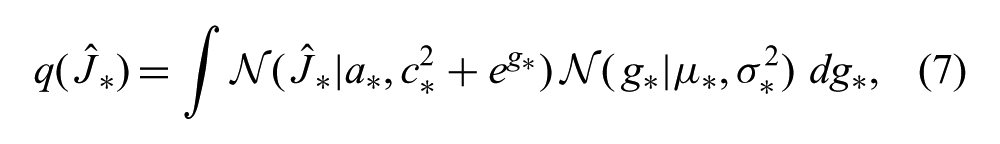
where

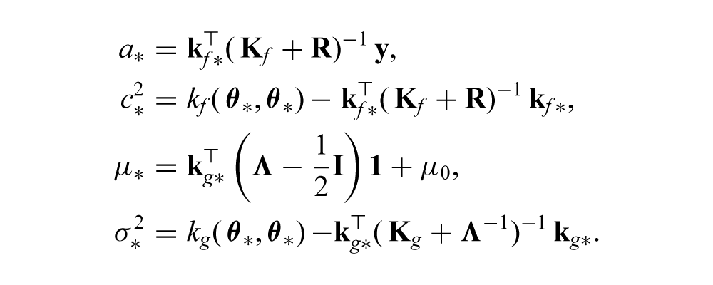
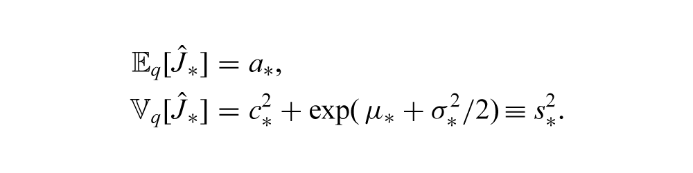
\begin{array}{l} a_{*} & = & k_{f *}^{⊤} {(K_{f} + R)}^{- 1} y, \\ c_{*}^{2} & = & k_{f} (θ_{*}, θ_{*}) - k_{f *}^{⊤} {(K_{f} + R)}^{- 1} k_{f *}, \\ μ_{*} & = & k_{g *}^{⊤} (Λ - \frac{1}{2} I) 1 + μ_{0}, \\ σ_{*}^{2} & = & k_{g} (θ_{*}, θ_{*}) - k_{g *}^{⊤} {(K_{g} + Λ^{- 1})}^{- 1} k_{g *} . \end{array}

Although this predictive density is intractable, its mean and variance can be calculated in closed form:

\begin{array}{l} E_{q} [{\hat{J}}_{*}] & = & a_{*}, \\ V_{q} [{\hat{J}}_{*}] & = & c_{*}^{2} + exp (μ_{*} + σ_{*}^{2} / 2) \equiv s_{*}^{2} . \end{array}

2.2.1. Example

Figure 1(a) shows the result of performing model selection given a GP prior with a squared exponential kernel and unknown constant noise variance on a synthetic heteroscedastic data set. Figure 1(b) shows the result of optimizing the VHGP model on the same data. Model selection was performed using SQP to maximize the marginal log likelihood or, in the case of the VHGP model, the marginal variational bound (6). Owing to the constant noise assumption, the GP model overestimates the cost variance in regions of low variance and underestimates in regions of high variance. In contrast, the VHGP model captures the input-dependent noise structure.

Fig. 1.

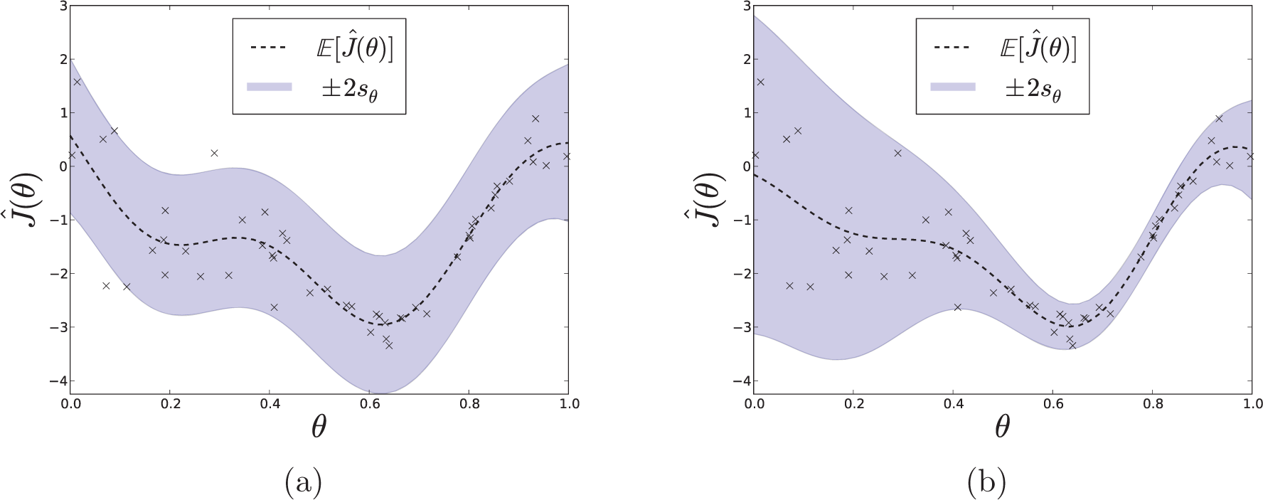
Comparison of fits for the standard GP model (a) and the VHGP model (b) on a synthetic heteroscedastic data set.

3. Variational Bayesian optimization

There are at least two practical motivations for modifying Bayesian optimization to capture policy-dependent cost variance. The first reason is to enable metrics computed on the predictive distribution, such as EI or probability of improvement, to return more meaningful values for the problem under consideration. For example, the GP model in Figure 1 would overestimate the EI for θ = 0.6 and underestimate the EI of θ = 0.2. The second reason is that it creates the opportunity to employ policy selection criteria that take cost variance into account, i.e. that are risk-sensitive.

We extend the VHGP model to the optimization case by deriving the expression for EI and its gradients and show that both can be efficiently approximated to several decimal places using Gauss–Hermite quadrature (as is the case for the predictive distribution itself (Lázaro-Gredilla and Titsias, 2011)). Efficiently computable CB selection criteria are also considered for selecting greedy risk-sensitive policies. A generalization of EI, called ERI, is derived that balances exploration and exploitation in the risk-sensitive case. Finally, to address numerical issues that arise when N is small (i.e. in the early stages of optimization), independent log priors are added to the marginal variational bound and heuristic sampling strategies are identified.

3.1. Expected improvement

Recall from Section 2.1.2 that the EI is defined as the expected reduction in cost, or improvement, over the average cost of the best policy previously evaluated. The probability of the policy parameters, θ _*, having improvement, I_*, under the variational predictive distribution (7) is

q (I_{*}) = \int N (I_{*} | μ_{best} - a_{*}, v_{*}^{2}) N (g_{*} | μ_{*}, σ_{*}^{2}) d g_{*},

where $v_{*}^{2} = c_{*}^{2} + e^{g *}$ . The expression for EI then becomes

\begin{array}{l} EI (θ_{*}) & = & \int_{0}^{\infty} I_{*} q (I_{*}) d I_{*} \\ = & \int_{0}^{\infty} \int I_{*} N (I_{*} | μ_{best} - a_{*}, v_{*}^{2}) \\ N (g_{*} | μ_{*}, σ_{*}^{2}) d g_{*} d I_{*} . \end{array}

(8)

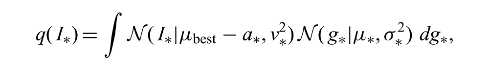
To get (8) into a more convenient form, we can define

u_{*} = \frac{μ_{best} - a_{*}}{v_{*}}, x_{*} = \frac{{\hat{J}}_{*} - a_{*}}{v_{*}},

and rewrite the expression for improvement (3) as

I_{*} = {\begin{matrix} v_{*} (u_{*} - x_{*}) & if x_{*} < u_{*}, \\ 0 & otherwise . \end{matrix}

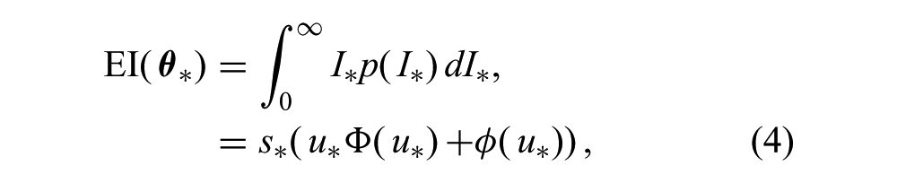
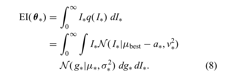
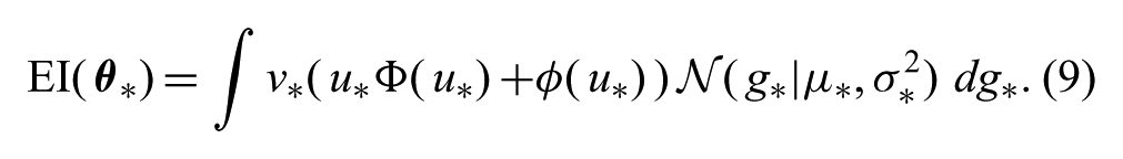
By using this alternative form of improvement and changing the order of integration, we have

EI (θ_{*}) = \int \int_{- \infty}^{u_{*}} v_{*} (u_{*} - x_{*}) φ (x_{*}) d x_{*} N (g_{*} | μ_{*}, σ_{*}^{2}) d g_{*} .

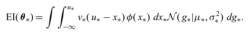
where ɸ(⋅) is the PDF of the normal distribution. Letting f(x_*) = v_*(u_*−x_*) and integrating $\int_{- \infty}^{u_{*}} f (x_{*}) φ (x_{*}) d x_{*}$ by parts, we have

\begin{array}{l} \int_{- \infty}^{u_{*}} f (x_{*}) φ (x_{*}) d x_{*} & = & {[f (x_{*}) Φ (x_{*})]}_{- \infty}^{u_{*}} \\ - \int_{- \infty}^{u_{*}} (- v_{*}) Φ (x_{*}) d x_{*}, \\ = & v_{*} {[x_{*} Φ (x_{*}) + φ (x_{*})]}_{- \infty}^{u_{*}}, \\ = & v_{*} (u_{*} Φ (u_{*}) + φ (u_{*})), \end{array}

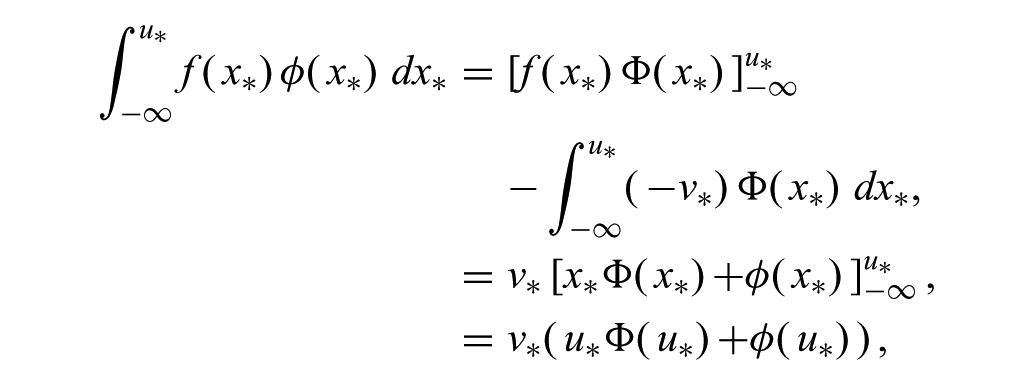
where we have used the facts that ${lim}_{x_{*} \to - \infty} φ (x_{*}) = 0$ and ${lim}_{x_{*} \to - \infty} C x_{*} Φ (x_{*}) = 0$ , where C is an arbitrary constant. Thus, the expression for EI is

EI (θ_{*}) = \int v_{*} (u_{*} Φ (u_{*}) + φ (u_{*})) N (g_{*} | μ_{*}, σ_{*}^{2}) d g_{*} .

(9)

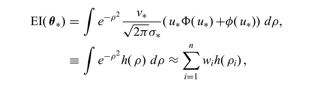
Although this expression is not analytically tractable, it can be efficiently approximated using Gauss–Hermite quadrature (Abramowitz and Stegun, 1972). This can be made clear by setting $ρ = (g_{*} - μ_{*}) / \sqrt{2} σ_{*}$ and replacing all occurrences of g_* in the expressions for v_* and u_*,

\begin{array}{l} EI (θ_{*}) & = & \int e^{- ρ^{2}} \frac{v_{*}}{\sqrt{2 π} σ_{*}} (u_{*} Φ (u_{*}) + φ (u_{*})) d ρ, \\ \equiv & \int e^{- ρ^{2}} h (ρ) d ρ \approx \sum_{i = 1}^{n} w_{i} h (ρ_{i}), \end{array}

where n is the number of sample points, ρ_i are the roots of the Hermite polynomial,

H_{n} (ρ) = {(- 1)}^{n} e^{ρ^{2}} \frac{d^{n} e^{- ρ^{2}}}{d ρ^{n}}, i \in {1, 2, \dots, n},

and the weights are computed as

w_{i} = \frac{2^{n - 1} n! \sqrt{π}}{n^{2} H_{n - 1} {(ρ_{i})}^{2}} .

In practice, a variety of tools are available for efficiently computing both w_i and ρ_i for a given n. In all of our experiments, n = 45.

Similarly, the gradient ∂EI ( θ ) / ∂ θ can be computed under the integral (9) and the result is of the desired form:

\frac{\partial EI (θ_{*})}{\partial θ} = \int e^{- ρ^{2}} z (ρ) d ρ,

where

\begin{array}{l} z (ρ) & = & \frac{1}{\sqrt{2 π} σ_{*}} [\frac{1}{σ_{*}} v_{*} (u_{*} Φ (u_{*}) + φ (u_{*})) \\ \times (- \frac{\partial σ_{*}}{\partial θ} + 2 ρ^{2} \frac{\partial σ_{*}}{\partial θ} + \sqrt{2} ρ \frac{\partial μ_{*}}{\partial θ}) \\ + \frac{\partial v_{*}}{\partial θ} (u_{*} Φ (u_{*}) + φ (u_{*})) + v_{*} \frac{\partial u_{*}}{\partial θ} Φ (u_{*})] . \end{array}

As in the standard Bayesian optimization setting, one can easily incorporate an exploration parameter, ξ, by setting u_* = (μ_best −a_* + ξ)/v_*, and maximize EI using standard nonlinear optimization algorithms. Since flat regions and multiple local maxima may be present, it is common practice to perform random restarts during EI optimization to avoid low-quality solutions. In our experiments, we used the NLOPT (Johnson, 2011) implementation of SQP with 25 random restarts to optimize EI.

3.2. Confidence bound selection

In order to exploit cost variance information for policy selection, we must consider selection criteria that flexibly take cost variance into account. Although EI performs well during learning by balancing exploration and exploitation, it falls short in this regard since it always favors high variance (or uncertainty) among solutions with equivalent expected cost. In contrast, CB selection criteria allow one to directly specify the sensitivity to cost variance.

The family of CB selection criteria have the general form

CB (θ_{*}, κ) = E [{\hat{J}}_{*}] + b (V [{\hat{J}}_{*}], κ),

(10)

where b(⋅,⋅) is a function of the cost variance and a constant risk factor, κ, that controls the system’s sensitivity to risk. Such criteria have been extensively studied in the context of statistical global optimization (Cox and John, 1992; Srinivas et al., 2010) and economic decision making (Levy and Markowitz, 1979). Favorable regret bounds for sampling with CB criteria with $b (V [J_{*}], κ) = κ \sqrt{V [J_{*}]} \equiv κ s_{*}$ have also been derived for certain types of Bayesian optimization problems (Srinivas et al., 2010).

Interestingly, CB criteria have a strong connection to the exponential utility functions of risk-sensitive optimal control (Whittle, 1981, 1990). For example, consider the risk-sensitive optimal control objective function,

γ (θ_{*}, κ) = - 2 κ^{- 1} log E [e^{- \frac{1}{2} κ {\hat{J}}_{*}}] .

(11)

By taking the second-order Taylor expansion of (11) about $E [{\hat{J}}_{*}]$ , we have

γ (θ_{*}, κ) \approx E [{\hat{J}}_{*}] - \frac{1}{4} κ V [{\hat{J}}_{*}] .

Thus, policies selected according to a CB criterion with $b (V [{\hat{J}}_{*}], κ) = - \frac{1}{4} κ V [{\hat{J}}_{*}]$ can be viewed as approximate risk-sensitive optimal control solutions. Furthermore, because the selection is performed with respect to the predictive distribution, policies with different risk characteristics can be selected on-the-fly, without having to perform additional policy executions. This is a distinguishing property of this approach compared to other risk-sensitive control algorithms that must perform separate optimizations that require significant computation or additional policy executions to produce policies with different risk-sensitivity.

In practice, one typically sets $b (V [{\hat{J}}_{*}], κ) = κ \sqrt{V [{\hat{J}}_{*}]} = κ s_{*}$ so that terms of the same units are combined and the parameter κ has a straightforward interpretation. It is noteworthy that other functions of the mean and variance can also be used to form useful risk-sensitive criteria. For example, the Sharpe ratio, $SR = E [{\hat{J}}_{*}] / s_{*}$ , is a commonly used metric in financial analysis (Sharpe, 1966). Since the mean and variance of the VHGP model are analytically computable, extensions that optimize such criteria would be straightforward to implement.

3.3. Expected risk improvement

The primary advantage CB criteria offer is the ability to flexibly specify sensitivity to risk. However, CB criteria are greedy with respect to risk-sensitive objectives and therefore do not have the same exploratory quality as EI does for expected cost minimization. It is therefore natural to consider whether the EI criterion could be extended to perform risk-sensitive policy selection in a way that balances exploration and exploitation.

Schonlau et al. (1998) considered a generalization of EI where the improvement for θ _* was defined as

I_{*}^{ρ} = max {0, {(μ_{best} - {\hat{J}}_{*})}^{ρ}},

where ρ is an integer-valued parameter that affects the relative importance of large, low-probability improvements and small, high-probability improvements. Interestingly, the authors showed that for ρ = 2, $EI (θ_{*}, ρ) = E {[{\hat{J}}_{*}]}^{2} + V [{\hat{J}}_{*}]$ , which can be interpreted as a risk-seeking policy selection strategy. However, to perform balanced exploration in systems with more general risk-sensitivity, a different generalization of EI is needed.

To address this problem, we propose an ERI criterion. In this case, the risk improvement for the policy parameters θ _* is defined as

I_{*}^{κ} = {\begin{array}{l} μ_{best} + κ s_{best} - {\hat{J}}_{*} - κ s_{*} & if {\hat{J}}_{*} + κ s_{*} < μ_{best} + κ s_{best}, \\ 0 & otherwise, \end{array}

where

\begin{array}{l} i & = & arg {min}_{j = 1, \dots, N} E [\hat{J} (θ_{j})] + κ s (θ_{j}), \\ μ_{best} & = & E [\hat{J} (θ_{i})], \\ s_{best} & = & s (θ_{i}) . \end{array}

Intuitively, the risk improvement captures the reduction in the value of the risk-sensitive objective, $E [\hat{J}] + κ s$ , over the best policy previously evaluated. Following a similar derivation as for EI, the ERI under the variational distribution is

\begin{array}{l} ERI (θ_{*}) & = & \int_{0}^{\infty} I_{*}^{κ} q (I_{*}^{κ}) d I_{*}^{κ} \\ = & \int v_{*} (u_{*} Φ (u_{*}) + φ (u_{*})) N (g_{*} | μ_{*}, σ_{*}^{2}) d g_{*}, \end{array}

(12)

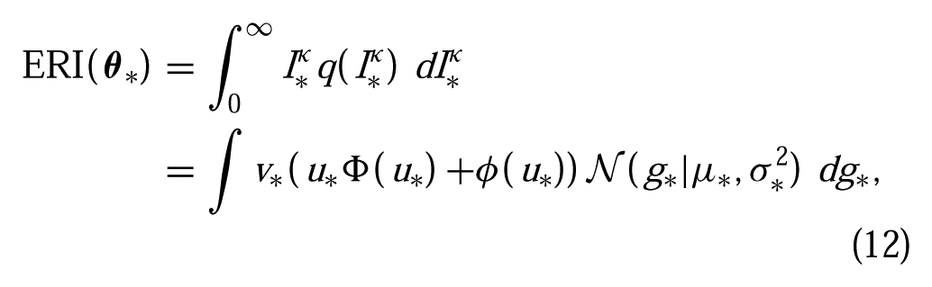
where u_* = (μ_best − a_* +κ(s_best − s_*))/v_*. Thus, ERI can be viewed as a straightforward generalization of EI, where ERI = EI if κ = 0.

3.4. Coping with small sample sizes

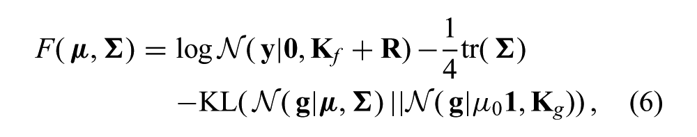
3.4.1. Log hyperpriors

Numerical precision problems are commonly experienced when performing model selection (which requires kernel matrix inversions and determinant calculations) using small amounts of data. To help improve numerical stability in the VHGP model when N is small, we augment F( μ , Σ) with independent log-normal priors for each hyperparameter,

\hat{F} (μ, Σ) = F (μ, Σ) + \sum_{ψ_{k} \in Ψ} log N (log ψ_{k} | μ_{k}, σ_{k}^{2}),

(13)

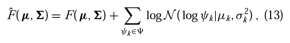
where Ψ = Ψ_f ∪ Ψ_g is the set of all hyperparameters. Lizotte et al. (2011) showed that empirical performance can be improved in the standard Bayesian optimization setting by incorporating log-normal hyperpriors into the model selection procedure. In practice, these priors can be quite vague and thus do not require significant experimenter insight. For example, in our experiments with variational Bayesian optimization (VBO), we set the log prior on length scales so that the width of the 95% confidence region is at least 20 times the actual policy parameter ranges.

As is the case with standard marginal likelihood maximization, $\hat{F} (μ, Σ)$ may have several local optima. In practice, performing random restarts helps avoid low-quality solutions (especially when N is small). In our experiments, SQP was used with 10 random restarts to perform model selection.

3.4.2. Sampling

It is well known that selecting policies based on distributions fit using very little data can lead to myopic sampling and premature convergence (Jones, 2001). For example, if one were unlucky enough to sample only the peaks of a periodic cost function, there would be good reason to infer that all policies have approximately equivalent cost. Incorporating external randomization is one way to help alleviate this problem. For example, it is common to obtain a random sample of N₀ initial policies prior to performing optimization. Sampling according to EI with probability 1−∊ and randomly otherwise can also perform well empirically. In the standard Bayesian optimization setting with model selection, ∊-random EI selection has been shown to yield near-optimal global convergence rates (Bull, 2011).

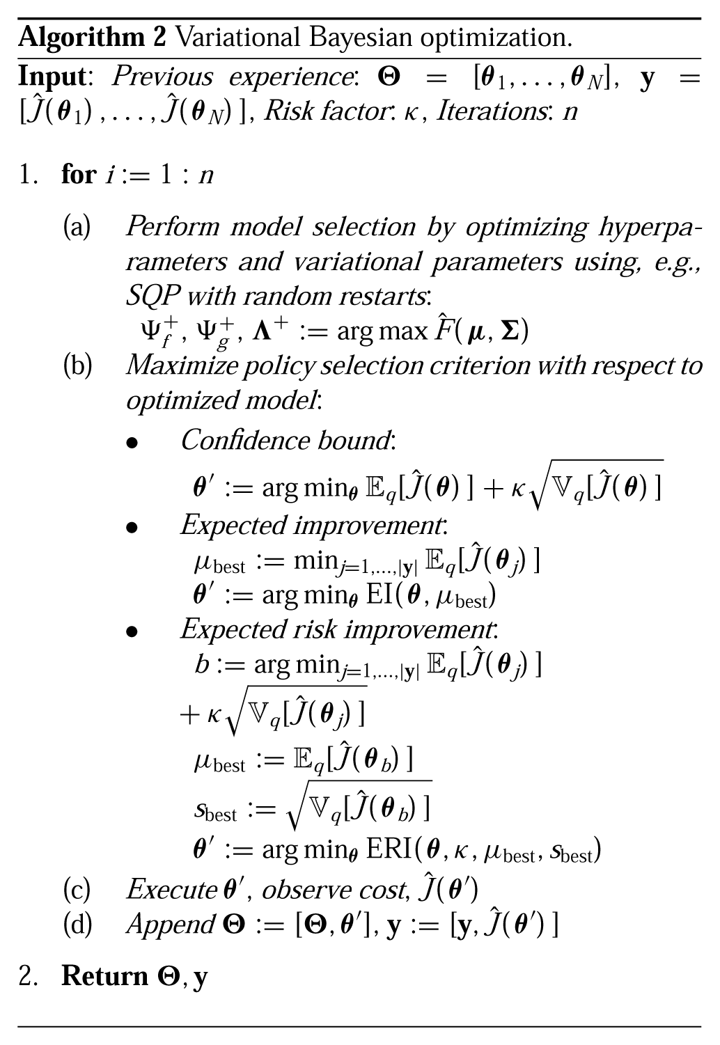
Randomized CB selection with, e.g., $κ ~ N (0, 1)$ can also be applied when the policy search is aimed at identifying a spectrum of policies with different risk-sensitivities. However, since this technique relies completely on the estimated cost distribution, it is most appropriate to apply after a reasonable initial estimate of the cost distribution has been obtained.

The VBO algorithm is shown in Algorithm 2.

Algorithm 2 Variational Bayesian optimization.
Input: Previous experience: $Θ = [θ_{1}, \dots, θ_{N}], y = [\hat{J} (θ_{1}), \dots, \hat{J} (θ_{N})]$ , Risk factor: κ, Iterations: n
1. for i:= 1: n
(a) Perform model selection by optimizing hyperparameters and variational parameters using, e.g., SQP with random restarts:
$Ψ_{f}^{+}$ , $Ψ_{g}^{+}$ , $Λ^{+} : = arg max \hat{F} (μ, Σ)$
(b) Maximize policy selection criterion with respect to optimized model:
• Confidence bound:
$θ^{'} : = arg {min}_{θ} E_{q} [\hat{J} (θ)] + κ \sqrt{V_{q} [\hat{J} (θ)]}$
• Expected improvement:
$μ_{best} : = {min}_{j = 1, \dots, \| y \|} E_{q} [\hat{J} (θ_{j})]$
θ ^′:= arg min_θEI ( θ , μ_best)
• Expected risk improvement:
$b : = arg {min}_{j = 1, \dots, \| y \|} E_{q} [\hat{J} (θ_{j})]$
$+ κ \sqrt{V_{q} [\hat{J} (θ_{j})]}$
$μ_{best} : = E_{q} [\hat{J} (θ_{b})]$
$s_{best} : = \sqrt{V_{q} [\hat{J} (θ_{b})]}$
θ ^′: = arg min_θ ERI ( θ , κ, μ_best, s_best)
(c) Execute θ ^′, observe cost, $\hat{J} (θ^{'})$
(d) Append Θ:= [Θ, θ ^′], $y : = [y, \hat{J} (θ^{'})]$
2. Return Θ, y

4. Local search

Like most standard Bayesian optimization implementations, no general global convergence guarantees exist for VBO. In addition, performing global selection of policy parameters can produce large jumps in policy space between trials, which can be undesirable in some physical systems. A straightforward way to address this latter concern is to restrict the parameter range to the local neighborhood of the nominal policy parameters. However, adding constraints in this way does not improve the convergence properties of the algorithm.

Gradient-based policy search methods make small, incremental changes to the policy parameters and typically have demonstrable local convergence properties under mild assumptions (Bertsekas and Tsitsiklis, 2000). Thus, in addition to using the learned cost model to perform global policy selection, we consider its use as a local critic for performing risk-sensitive gradient descent. It is straightforward to show that, under certain assumptions, the generalized RSSGD update follows the direction of the gradient of a CB objective. In addition, when a minimum variance baseline is used, the algorithm can be viewed as taking local steps in the direction of the risk improvement (Section 3.3) over the current policy parameters. This creates the opportunity to flexibly interweave risk-sensitive gradient descent and local VBO to, e.g., select local greedy policies or to change risk-sensitivity on-the-fly.

4.1. RSSGD

Stochastic gradient descent methods have had significant practical applicability to solving robot control problems in the expected cost setting (Kohl and Stone, 2004; Tedrake et al., 2004; Roberts and Tedrake, 2009), so we focus on extending this approach to the risk-sensitive case. The stochastic gradient descent algorithm, also called the weight perturbation algorithm (Jabri and Flower, 1992), is a simple method for descending the gradient of a noisy objective function. The algorithm proceeds as follows. Starting with parameters, θ , execute the policy, π_θ, and observe the cost, $\hat{J} (θ) \equiv {\hat{J}}_{θ}$ . Next, randomly sample a parameter perturbation, $z ~ N (0, σ^{2} I)$ , execute the perturbed policy, π_{θ
+z}, and observe the cost, $\hat{J} (θ + z) \equiv {\hat{J}}_{θ + z}$ . Finally, update the policy parameters, θ ← θ + Δ θ , where

Δ θ = - η ({\hat{J}}_{θ + z} - {\hat{J}}_{θ}) z,

and η is a step size parameter. Intuitively, this rule updates the parameters in the direction of z if ${\hat{J}}_{θ + z} < {\hat{J}}_{θ}$ , and in the direction of −z if ${\hat{J}}_{θ + z} > {\hat{J}}_{θ}$ . It can be shown that, in expectation, this update follows the true (scaled) gradient of the expected cost,

E [Δ θ] = - η σ^{2} \nabla E [{\hat{J}}_{θ}],

where $\nabla f_{θ} \equiv {\frac{\partial f}{\partial θ} |}_{θ}$ .

In contrast, consider the RSSGD update

Δ θ = - η ({\hat{J}}_{θ + z} + κ {\tilde{r}}_{θ + z} - b (θ)) z,

(14)

where ${\tilde{r}}_{θ + z}$ is an estimate of the cost standard deviation of π_{θ
+z} and b( θ ) is an arbitrary baseline function (Williams, 1992) of the policy parameters.

Substituting (5) into (14) and taking the first-order Taylor expansion at θ + z, we have

\begin{array}{l} Δ θ & = & - η (J_{θ + z} + ε_{θ + z} + κ {\tilde{r}}_{θ + z} - b (θ)) z, \\ \approx & - η (J_{θ} + z^{⊤} \nabla J_{θ} + ε_{θ} + u z^{⊤} \nabla r_{θ} \\ + κ {\tilde{r}}_{θ} + κ z^{⊤} \nabla {\tilde{r}}_{θ} - b (θ)) z, \\ \equiv & \tilde{Δ} θ, \end{array}

where $u ~ N (0, 1)$ . In expectation, this becomes

E [\tilde{Δ} θ] = - η σ^{2} (\nabla J_{θ} + κ \nabla {\tilde{r}}_{θ}),

(15)

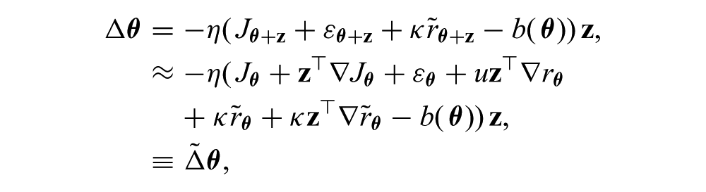
where the expectation is taken with respect to z, u, and ε_θ. Thus, the update equation (14) is an estimator of the gradient of expected cost that is biased in the direction of the estimated gradient of the standard deviation (to a degree specified by the risk factor κ). If the estimator of the cost standard deviation is unbiased, we have

E [\tilde{Δ} θ] = - η σ^{2} \nabla CB (θ, κ),

(16)

a scaled unbiased estimate of the gradient of the CB objective, CB ( θ , κ) = J_θ +κr_θ. Using a non-parametric model, such as VHGP, as a local critic will not, in general, lead to unbiased estimates of the mean and variance of the cost. However, by introducing bias these methods can potentially produce useful approximations of the local cost distribution after only a small number of policy evaluations.

4.1.1. Natural gradient

From (16) it is clear that the unbiasedness of the update is also dependent on the isotropy of the sampling distribution, $z ~ N (0, σ^{2} I)$ . However, as was shown by Roberts and Tedrake (2009), learning performance can be improved in some cases by optimizing the sampling distribution variance independently for each policy parameter, $z ~ N (0, Σ)$ . In this case, the expected update becomes biased,

E [\tilde{Δ} θ] = - η Σ \nabla CB (θ, κ),

(17)

but it is still in the direction of the natural gradient (Amari, 1998). To see this, recall that for probabilistically sampled policies, the natural gradient is defined as F⁻¹∇f ( θ ), where F⁻¹ is the inverse Fisher information matrix (Kakade, 2002). When the policy sampling distribution is mean-zero Gaussian with covariance Σ, the inverse Fisher information matrix is F⁻¹ = Σ. Thus, (17) is in the direction of the natural gradient.

4.1.2. Baseline selection

The expected update (15) is unaffected by the choice of the baseline function, b( θ ), given that it depends only on θ . However, the choice of baseline does affect the variance of the update. The variance of the update (14) can be written as

\begin{array}{l} V [\tilde{Δ} θ] & = & η^{2} σ^{2} (b {(θ)}^{2} I - 2 J_{θ} b (θ) I - 2 κ {\tilde{r}}_{θ} b (θ) I \\ + J_{θ}^{2} I + 2 κ J_{θ} {\tilde{r}}_{θ} I + κ^{2} {\tilde{r}}_{θ}^{2} I + r_{θ}^{4} I \\ + σ^{2} (\nabla J_{θ}^{⊤} \nabla J_{θ} I + \nabla J_{θ} \nabla J_{θ}^{⊤}) \\ + σ^{2} κ (2 \nabla J_{θ}^{⊤} \nabla {\tilde{r}}_{θ} I + \nabla J_{θ} \nabla {\tilde{r}}_{θ}^{⊤} + \nabla {\tilde{r}}_{θ} \nabla J_{θ}^{⊤}) \\ + σ^{2} r_{θ}^{2} (\nabla r_{θ}^{⊤} \nabla r_{θ} I + 2 \nabla r_{θ} \nabla r_{θ}^{⊤}) \\ + σ^{2} κ^{2} (\nabla {\tilde{r}}_{θ}^{⊤} \nabla {\tilde{r}}_{θ} I + \nabla {\tilde{r}}_{θ} \nabla {\tilde{r}}_{θ}^{⊤})) . \end{array}

(18)

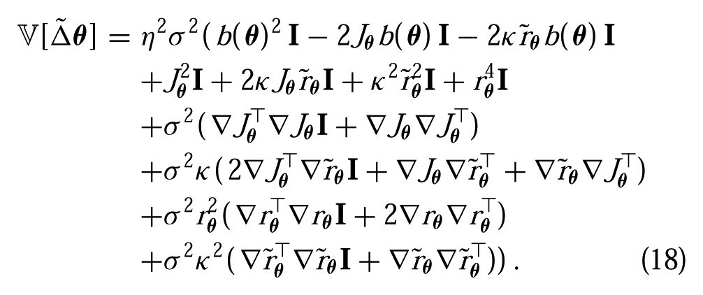
It is straightforward to show that the baseline that minimizes (18) is $b (θ) = J_{θ} + κ {\tilde{r}}_{θ}$ . However, since J_θ is unknown, we define the baseline using an estimate of the expected cost, ${\tilde{J}}_{θ}$ . The resulting increase in variance over the optimal baseline is proportional to the squared error of the expected cost estimate: $η^{2} σ^{2} {(J_{θ} - {\tilde{J}}_{θ})}^{2}$ . The RSSGD update then becomes

Δ θ = - η ({\hat{J}}_{θ + z} - {\tilde{J}}_{θ} + κ ({\tilde{r}}_{θ + z} - {\tilde{r}}_{θ})) z .

(19)

Intuitively, Equation (19) reduces to the classical stochastic gradient descent update when either the system has a neutral attitude toward risk (κ = 0) or when the estimate of the cost standard deviation is locally constant: $\nabla {\tilde{r}}_{θ} = 0 \Rightarrow {\tilde{r}}_{θ + z} - {\tilde{r}}_{θ} = 0$ , for small z such that the linearization holds. Note the relationship between the RSSGD update and the ERI criterion (12). From this point of view, the update can be interpreted as taking steps in the direction of risk improvement over the nominal policy parameter setting.

In implementation, it can be helpful to divide the step size by ${\tilde{r}}_{θ}$ so the update maintains scale invariance to changing noise magnitude (see Algorithm 3). In this way, samples are weighted by the local cost variance estimate so, e.g., large differences in cost in high-variance regions do not cause large fluctuations in the policy parameter values. On the other hand, large fluctuations in the cost variance estimate could produce undesirably large or small step sizes. We therefore also constrain the scaled step size to stay in some reasonable range, e.g., $η / {\tilde{r}}_{θ} \in [0.01, 0.9]$ . Although this approach is heuristic, it does have practical advantages such as weighting updates according to their perceived reliability.

Algorithm 3 Risk-sensitive stochastic gradient descent.
Input: Parameters: η, σ, ε, Risk factor: κ, Initial policy: θ
1. Initialize Θ = [ ], y = [ ],
2. while not converged:
(a) Sample perturbation: $z ~ N (0, σ^{2} I)$
(b) Execute θ + z, record cost ${\hat{J}}_{θ + z}$
(c) Update data:
$Θ, y = [Θ, θ + z], [y, {\hat{J}}_{θ + z}]$
Θ_loc, y_loc = NearestNeighbors(Θ, y, θ , ∊)
(d) Compute posterior mean and variance:
${\tilde{J}}_{θ} = E [{\hat{J}}_{θ} Θ_{loc}, y_{loc}]$
${\tilde{r}}_{θ}^{2} = V [{\hat{J}}_{θ} Θ_{loc}, y_{loc}]$
${\tilde{r}}_{θ + z}^{2} = V [{\hat{J}}_{θ + z} Θ_{loc}, y_{loc}]$
(e) Update policy parameters:
$Δ θ : = - \frac{η}{{\tilde{r}}_{θ}} ({\hat{J}}_{θ + z} - {\tilde{J}}_{θ} + κ ({\tilde{r}}_{θ + z} - {\tilde{r}}_{θ})) z$
θ := θ + Δ θ
3. Return Θ, y, θ

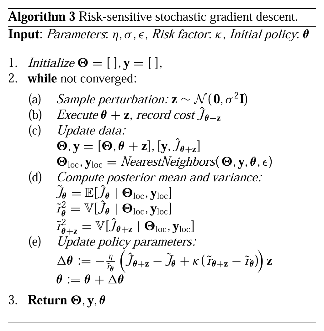
As in VBO, the critic is updated after each policy evaluation by recomputing the predictive cost distribution. However, in this case model selection and prediction are performed using only observations near the current parameterization, θ . A nearest-neighbor selection can be performed efficiently around the current policy parameters by storing observations in a k d-tree data structure and using, e.g., a k-nearest neighbors or an ∊-ball criterion. However, because the number of samples is typically small in the types of robot control tasks under consideration, the actual computational effort required to find nearest neighbors and perform model selection is quite modest. Thus, the primary advantage of constructing a local, rather than a global, model is that cost distributions that are non-stationary with respect to their optimal hyperparameter values can be handled more easily. The RSSGD algorithm is outlined in Algorithm 3.

5. Experiments

In Sections 5.1 and 5.2 we illustrate the VBO algorithm using simple synthetic domains. In Section 5.3, we apply VBO to a impact recovery task with the uBot-5 mobile manipulator. Finally, in Section 5.4, we apply the RSSGD algorithm in a dynamic heavy lifting task with the uBot-5.

5.1. Synthetic data

As an illustrative example, in Figure 2 we compare the performance of VBO to standard Bayesian optimization in a simple one-dimensional noisy optimization task. For this task, the true underlying cost distribution (Figure 2(a)) has two global minima (in the expected cost sense) with different cost variances. Both algorithms begin with the same N₀ = 10 random samples and perform 10 iterations of EI selection (ξ = 1.0, ∊ = 0.25). In Figure 2(b), we see that Bayesian optimization succeeds in identifying the regions of low cost, but it cannot capture the policy-dependent variance characteristics.

Fig. 2.

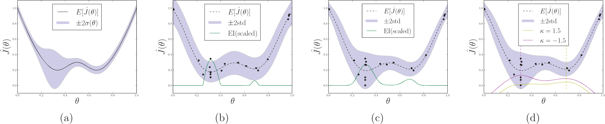
(a) An example unknown noise distribution with two equivalent expected cost minima with different cost variance. (b) The distribution learned after 10 iterations of Bayesian optimization with EI selection and (c) after 10 iterations of VBO with EI selection (using the same initial N₀ = 10 random samples for both cases). Bayesian optimization succeeded in identifying the minima, but it cannot distinguish between high- and low-variance solutions. (d) CB selection criteria are applied to select risk-seeking and risk-averse policy parameters (indicated by the vertical dotted lines) given the distribution learned using VBO.

In contrast, VBO reliably identifies the minima and approximates the local variance characteristics. Figure 2(d) shows the result of applying two different CB selection criteria to vary risk-sensitivity. In this case, −CB ( θ _*,κ) was maximized, where

CB (θ_{*}, κ) = E_{q} [{\hat{J}}_{*}] + κ s_{*} .

(20)

Risk factors κ = −1.5 and κ = 1.5 were used to select a risk-seeking and risk-averse policy parameters, respectively.

5.2. Noisy pendulum

As another simple example, we considered a swing-up task for a noisy pendulum system. In this task, the maximum torque output of the pendulum actuator is unknown and is drawn from a normal distribution at the beginning of each episode. As a rough physical analogy, this might be understood as fluctuations in motor performance that are caused by unmeasured changes in temperature. The policy space consisted of “bang–bang” policies in which the maximum torque is applied in the positive or negative direction, with switching times specified by two parameters, 0 ≤ t₁, t₂ ≤ 1.5 s. Thus, θ = [t₁, t₂]. The cost function was defined as

J (θ) = \int_{0}^{T} 0 . 01 α (t) + 0.0001 u {(t)}^{2} d t,

(21)

where 0 ≤ α (t) ≤ π is the pendulum angle measured from upright vertical, T = 3.5 s, and u(t) = τ_max if 0 ≤ t ≤ θ₁, u(t) = −τ_max if θ₁ < t ≤ θ₁ +θ₂, and u(t) = τ_max if θ₁ +θ₂ < t ≤ T. The system always started in the downward vertical position with zero initial velocity and the episode terminated if the pendulum came within 0.1 rad of the upright vertical position. The parameters of the system were l = 1.0 m, m = 1.0 kg, and $τ_{max} ~ N (4, {0.3}^{2}) Nm$ . With these physical parameters, the pendulum must (with probability ≈ 1.0) perform at least two swings to reach vertical in less than T seconds.

The cost function (21) suggests that policies that reach vertical as quickly as possible (i.e. using the fewest swings) are preferred. However, the success of an aggressive policy depends on the torque generating capability of the pendulum. With a noisy actuator, it is reasonable to expect aggressive policies to have higher variance. An approximation of the cost distribution obtained via discretization (N = 40,000) is shown in Figure 3(a). 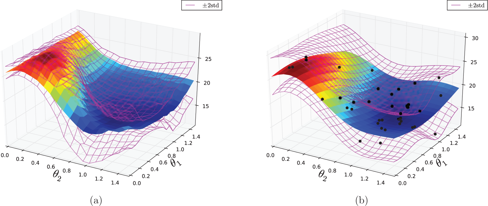It is clear from this figure that regions around policies that attempt two-swing solutions ( θ = [0.0, 1.0], θ = [1.0, 1.5]) have low expected cost, but high cost variance.

Fig. 3.

(a) The cost distribution for the simulated noisy pendulum system obtained by a 20 × 20 discretization of the policy space. Each policy was evaluated 100 times to estimate the mean and variance (N = 40,000). (b) Estimated cost distribution after 25 iterations of VBO with 15 initial random samples (N = 40). Owing to the sample bias that results from EI selection, the optimization algorithm tends to focus modeling effort in regions of low cost.

Figure 3(b) shows the results of 25 iterations of VBO using EI selection (N₀ = 15, ξ = 1.0, ∊ = 0.2) in the noisy pendulum task. After N = 40 total evaluations, the expected cost and cost variance are sensibly represented in regions of low cost. Figure 4 illustrates the behavior of two policies selected by minimizing the CB criterion (20) on the learned distribution with κ = ±2.0. 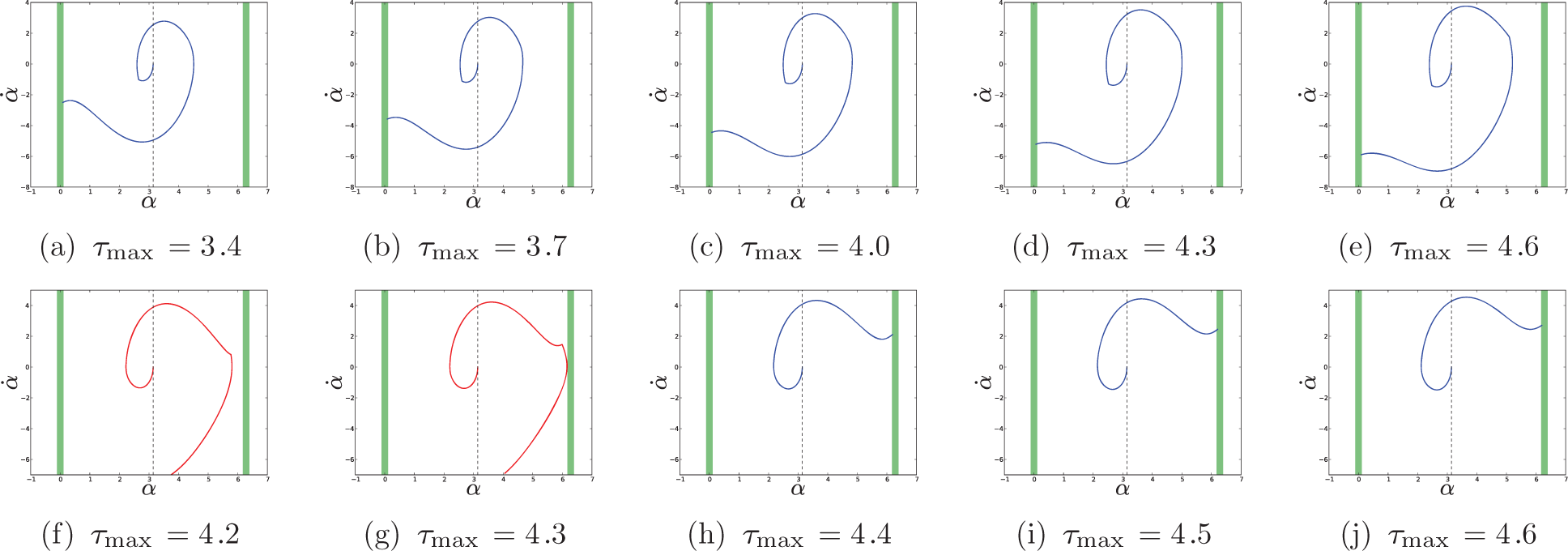The risk-seeking policy ( θ = [1.03, 1.5]) makes a large initial swing, attempting to reach the vertical position in two swings. In doing so, it only succeeds in reaching the goal configuration when the unobserved maximum actuator torque is large (roughly $E [τ_{max}] + σ [τ_{max}]$ ). The risk-averse policy ( θ = [0.63, 1.14]) always produces three swings and exhibits low cost variance, although it has higher cost than the risk-seeking policy when the maximum torque is large (15.93 versus 13.03).

Fig. 4.

Performance of risk-averse (a)–(e) and risk-seeking (f)–(j) policies as the maximum pendulum torque is varied. Shown are phase plots with the goal regions shaded in green. The risk-averse policy always used three swings and consistently reached the vertical position before the end of the episode. The risk-seeking policy used longer swing durations, attempting to reach the vertical position in only two swings. However, this strategy only pays off when the unobserved maximum actuator torque is large.

It is often easy to understand the utility of risk-averse and risk-neutral policies, but the motivation for selecting risk-seeking policies might be less clear. The above result suggests one possibility: the acquisition of specialized, high-performance policies. For example, in some cases risk-seeking policies could be chosen in an attempt to identify observable initial conditions that lead to rare low-cost events. Subsequent optimizations might then be performed to direct the system to these initial conditions. One could also imagine situations when the context demands performance that lower risk policies are very unlikely to generate. For example, if the minimum time to goal was reduced so that only two swing policies had a reasonable chance of succeeding. In such instances it may be desirable to select higher-risk policies, even if the probability of succeeding is quite low.

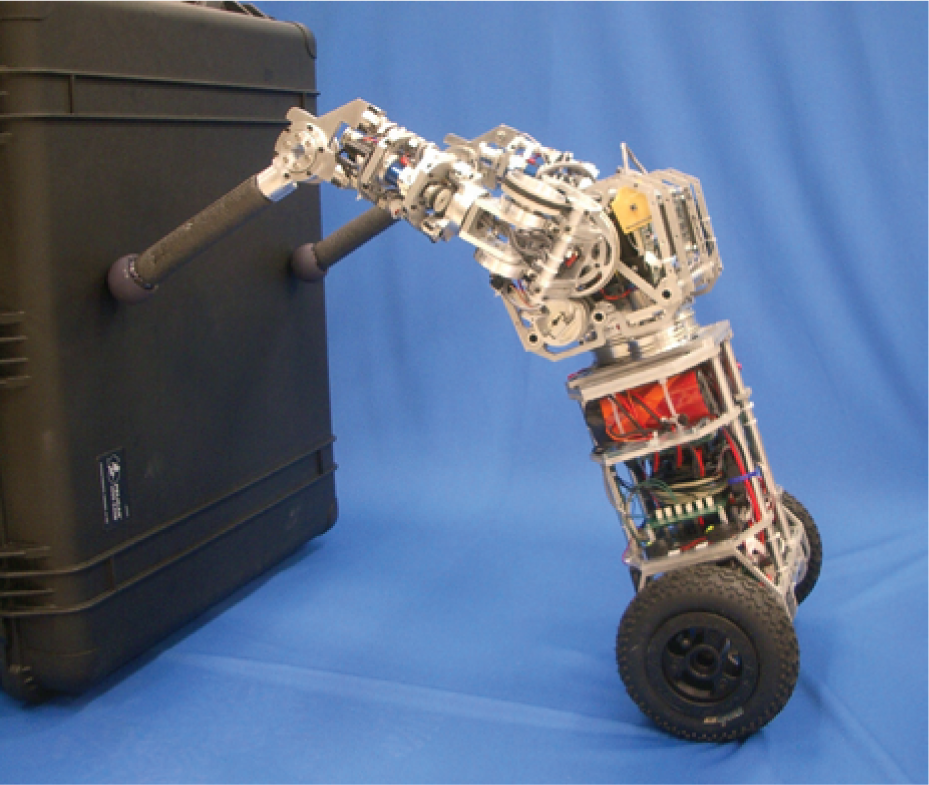
5.3. Balance recovery with the uBot-5

The uBot-5 (Figure 5) is an 11-degree-of-freedom (11-DoF) mobile manipulator developed at the University of Massachusetts Amherst (Kuindersma et al., 2009; Deegan, 2010). The uBot-5 has two 4-DoF arms, a rotating trunk, and two wheels in a differential drive configuration. The robot stands approximately 60 cm from the ground and has a total mass of 19 kg. The robot’s torso is roughly similar to an adult human in terms of geometry and scale, but instead of legs, it has two wheels attached at the hip. The robot balances using a linear-quadratic regulator (LQR) with feedback from an onboard inertial measurement unit (IMU) to stabilize around the vertical fixed point. The LQR controller has proved to be very robust throughout 5 years of frequent usage and it remains fixed in our experiments.

Fig. 5.

The uBot-5 demonstrating a whole-body pushing behavior.

In our previous experiments (Kuindersma et al., 2011), the energetic and stabilizing effects of rapid arm motions on the LQR stabilized system were evaluated in the context of recovery from impact perturbations. One observation made was that high-energy impacts caused a subset of possible recovery policies to have high cost variance: successfully stabilizing in some trials, while failing to stabilize in others. We extended these experiments by considering larger impact perturbations, increasing the set of arm initial conditions, and defining a policy space that permits more flexible, asymmetric arm motions (Kuindersma et al., 2012b).

The robot was placed in a balancing configuration with its upper torso aligned with a 3.3 kg mass suspended from the ceiling (Figure 6). The mass was pulled away from the robot to a fixed angle and released, producing a controlled impact between the swinging mass and the robot. The pendulum momentum prior to impact was 9.9 ± 0.8 Ns and the resulting impact force was approximately equal to the robot’s total mass in Earth’s gravity. The robot was consistently unable to recover from this perturbation using only the wheel LQR (see the rightmost column of Figure 7). The robot was attached to the ceiling with a loose-fitting safety rig designed to prevent the robot from falling completely to the ground, while not affecting policy performance.

Fig. 6.

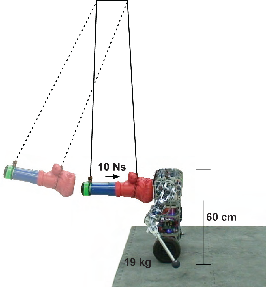
The uBot-5 situated in the impact pendulum apparatus.

Fig. 7.

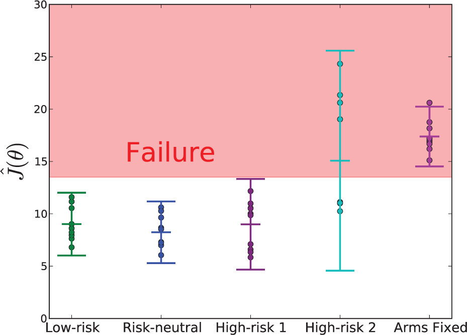
Data collected over 10 trials using policies identified as risk-averse, risk-neutral, and risk-seeking after performing VBO. The policies were selected using CB criteria with κ = 2, κ = 0, κ = −1.5, and κ = −2, from left to right. The sample means and two times sample standard deviations are shown. The shaded region contains all trials that resulted in failure to stabilize. Ten trials with a fixed-arm policy are plotted on the far right to serve as a baseline level of performance for this impact magnitude.

This problem is well suited for model-free policy optimization since there are several physical properties, such as joint friction, wheel backlash, and tire slippage, that make the system difficult to model accurately. In addition, although the underlying state and action spaces are high-dimensional (22 and 8, respectively), low-dimensional policy spaces that contain high-quality solutions are relatively straightforward to identify.

The parameterized policy controlled each arm joint according to an exponential trajectory, τ_i(t) = e^−λit, where 0 ≤ τ_i (t) ≤ 1 is the commanded DC motor power for joint i at time t. The λ parameters were paired for the shoulder/elbow pitch and the shoulder roll/yaw joints. This pairing allowed the magnitude of dorsal and lateral arm motions to be independently specified. The pitch (dorsal) motions were specified separately for each arm and the lateral motions were mirrored, which reduced the number of policy parameters to three. The range of each λ_i was constrained: 1 ≤ λ_i ≤ 15. 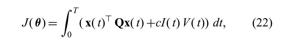At time t, if $\forall_{i} τ_{i} (t) < 0.25$ , the arms were retracted to a nominal configuration (the mean of the initial configurations) using a fixed, low-gain linear position controller.

The cost function was designed to encourage energy-efficient solutions that successfully stabilized the system:

J (θ) = h (x (T)) + \int_{0}^{T} \frac{1}{10} I (t) V (t) d t,

where I(t) and V (t) are the total absolute motor current and voltage at time t, respectively, T = 3.5 s, and h(x(T)) = 5 if x(T) ∈ FailureStates, otherwise h(x(T)) = 0. After 15 random initial trials, we applied VBO with EI selection (ξ = 1.0,∊ = 0.2) for 15 episodes and randomized CB selection ( $κ ~ N (0, 1)$ ) for 15 episodes resulting in a total of N = 45 policy evaluations (approximately 2.5 minutes of total experience). Since the left and right pitch parameters are symmetric with respect to cost, we imposed an arbitrary ordering constraint, λ_left ≥ λ_right, during policy selection.

After training, we evaluated four policies with different risk-sensitivities selected by minimizing the CB criterion (20) with κ = 2, κ = 0, κ = −1.5, and κ = −2. Each selected policy was evaluated 10 times and the results are shown in Figure 7. The sample statistics confirm the algorithmic predictions about the relative riskiness of each policy. In this case, the risk-averse and risk-neutral policies were very similar (no statistically significant difference between the mean or variance), while the two risk-seeking policies had higher variance (for κ = −2, the differences in both the sample mean and variance were statistically significant).

For κ = −2, the selected policy produced an upward laterally directed arm motion that failed approximately 50% of the time. In this case, the standard deviation of cost was sufficiently large that the second term in CB objective (20) dominated, producing a policy with high variance and poor average performance. A slightly less risk-seeking selection (κ = −1.5) yielded a policy with conservative low-energy arm movements that was more sensitive to initial conditions than the lower risk policies. This exertion of minimal effort could be viewed as a kind of gamble on initial conditions. Figure 8 shows example runs of the risk-averse and risk-seeking policies.

Fig. 8.

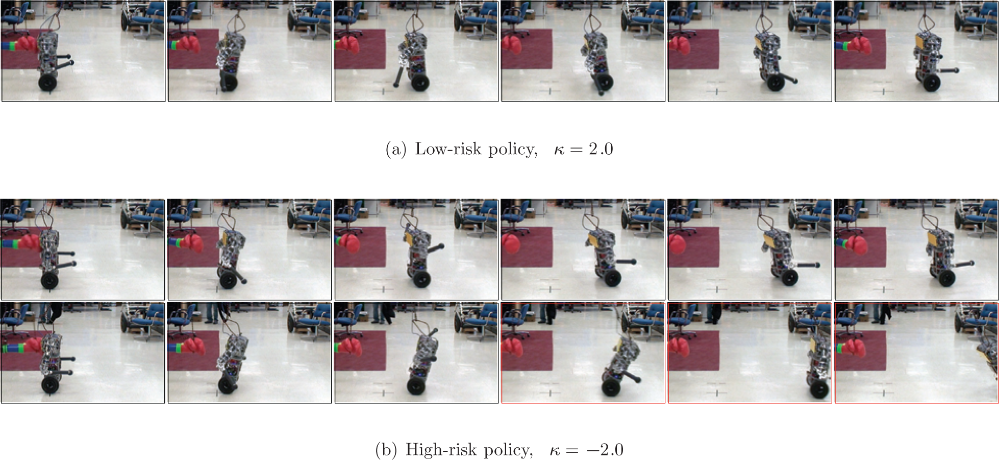
Time series (time between frames is 0.24 seconds) showing (a) a trial executing the low-risk policy and (b) two trials executing the high-risk policy. Both policies were selected using CB criteria on the learned cost distribution. The low-risk policy produced an asymmetric dorsally directed arm motion with reliable recovery performance. The high-risk policy produced an upward laterally directed arm motion that failed approximately 50% of the time.

5.4. Dynamic heavy lifting

We evaluated the RSSGD algorithm in the dynamic control task of lifting a 1 kg, partially filled laundry detergent bottle from the ground to a height of 120 cm using the uBot-5 (Kuindersma et al., 2012a). This problem is challenging for several reasons. First, the bottle is heavy, so most arm trajectories from the starting configuration to the goal will not succeed because of the limited torque generating capabilities of the arm motors. Second, the upper body motions act as disturbances to the LQR. Thus, violent lifting trajectories will cause the robot to destabilize and fall. Finally, the bottle itself has significant dynamics because the heavy liquid sloshes as the bottle moves. Since the robot had only a simple claw gripper and we made no modifications to the bottle, the bottle moved freely in the hand, which had a significant effect on the stabilized system.

The policy was represented as a cubic spline trajectory in the right arm joint space with seven open parameters to be optimized by the algorithm. The parameters included four shoulder and elbow waypoint positions and three time parameters. The start and end configurations were fixed. Joint velocities at the waypoints were computed using the tangent method (Craig, 2005). The initial policy was a hand-crafted smooth and short duration motion to the goal configuration. Our ability to provide a good initial guess for the policy parameters makes local search with RSSGD more attractive. However, with the bottle in hand, this policy succeeded only a small fraction of the time, with most trials resulting in a failure to lift the bottle above the shoulder.

The cost function was defined as

J (θ) = \int_{0}^{T} (x {(t)}^{⊤} Q x (t) + c I (t) V (t)) d t,

(22)

where $x = {[x_{w h e e l}, {\dot{x}}_{w h e e l}, α_{b o d y}, {\dot{α}}_{b o d y}, h_{e r r o r}]}^{⊤}$ , I(t) and V (t) are total motor current and voltage for all motors at time t, Q = diag ([0.001, 0.001, 0.5, 0.5, 0.05]), and c = 0.01. The components of the state vector are the wheel position and velocity, body angle and angular velocity, and vertical error between the desired and actual bottle position, respectively. Intuitively, this cost function encourages fast and energy efficient solutions that do not violently perturb the LQR. In each trial, the sampling rate was 100 Hz and T = 6 s. A trial ended when either t > T or the robot reached the goal configuration with maintained low translational velocity (≤ 5 cm/s). The algorithm parameter values in all experiments were η = 0.5, σ = 0.075, ∊ = 3.5σ, and $η / {\tilde{r}}_{θ} \in [0.01, 0.5]$ . Each policy parameter range was scaled to be θ_i ∈ [0, 1], so the constant σ corresponded to different (unscaled) perturbation sizes for each dimension depending on the total parameter range.

5.4.1. Risk-neutral learning

In the first experiment, we ran RSSGD with κ = 0 to perform a risk-neutral gradient descent. The VHGP model was used to locally construct the critic and model selection was performed using SQP. A total of 30 trials (less than 2.5 minutes of total experience) were performed and a reliable, low-cost policy was learned. The robot failed to recover balance in 3 of the 30 trials. In these cases, the emergency stop was activated and the robot was manually reset. Figure 9 illustrates the reduction in cost via empirical measurements taken at fixed intervals during learning.

Fig. 9.

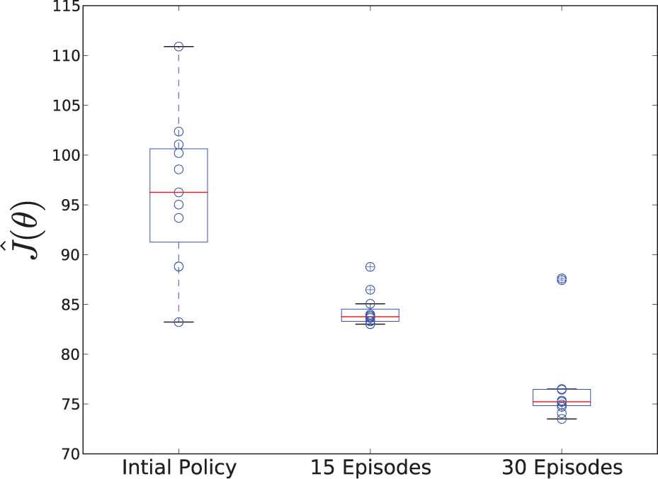
Data collected from 10 test trials executing the initial lifting policy and the policy after 15 and 30 episodes of learning.

Interestingly, the learned policy exploits the dynamics of the liquid in the bottle by timing the motion such that the shifting bottle contents coordinate with the LQR controller to correct the angular displacement of the body. This dynamic interaction would be very difficult to capture in a system model. Incidentally, this serves as a good example of the value of policy search techniques: by virtue of ignoring the dynamics, they are in some sense insensitive to the complexity of the dynamics (Roberts and Tedrake, 2009). Figure 10(a) shows an example run of the learned policy.

Fig. 10.

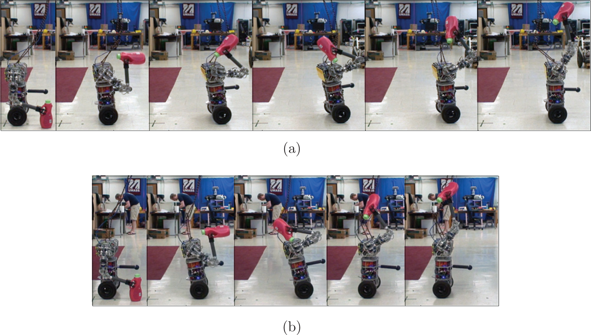
(a) The learned risk-neutral policy exploits the dynamics of the container to reliably perform the lifting task. (b) With no additional learning trials, a risk-averse policy is selected offline that reliably reduces translation. The total time duration of each of the above sequences is approximately 3 seconds.

5.4.2. Variable risk control

In the process of learning a low average-cost policy, a model of the local cost distribution was repeatedly computed. The next experiments examined the effect of performing offline policy selection using the estimate of the local cost distribution around the learned policy. In particular, we considered two hypothetical changes in operating context: when the robot’s workspace is reduced, requiring that the policy have a small footprint with high certainty, and when the battery charge is very low, requiring that the policy uses very little energy with high certainty. Offline CB policy selection and subsequent risk-averse gradient descent was performed for each case and the resulting policies were compared empirically.

Context changes were represented by a reweighting of cost function terms. For example, to capture the low-battery-charge context, the relative weight of the motor power term in (22) was increased: Q_en = diag ([0.0005, 0.0005, 0.25, 0.25, 0.05]) and c_en = 0.1. The cost of previous trajectories was then computed using the transformed cost function,

J_{e n} (θ) = \int_{0}^{T} (x {(t)}^{⊤} Q_{e n} x (t) + c_{e n} I (t) V (t)) d t .

(23)

The VHGP model was used to approximate the transformed cost distribution, ${\hat{J}}_{e n} (θ)$ , around the previously learned policy parameters using the data collected during the 30 learning trials. SQP was used to minimize ${\tilde{J}}_{e n} (θ) + κ {\tilde{r}}_{e n} (θ)$ offline. Likewise, to represent the translation-averse case, the relative weight assigned to wheel translation was increased, Q_tr = diag ([0.002, 0.001, 0.5, 0.5, 0.05]) and c_tr = 0.001, and the resulting transformed local model was used to minimize ${\tilde{J}}_{t r} (θ) + κ {\tilde{r}}_{t r} (θ)$ offline.

Both risk-neutral (κ = 0) and risk-averse (κ = 2) offline policy selections were performed for each case. In addition, five episodes of risk-averse (κ = 2) gradient descent were performed starting from the offline selected risk-averse policy. Each policy was executed five times and the results were compared empirically. Figure 11(a) shows the results from the translation aversion experiments. The risk-neutral offline policy had significantly lower average (transformed) cost and lower variance than the original learned policy. The risk-averse offline policy also has significantly lower average cost than the prior learned policy, but its average cost was slightly (not statistically significantly) higher than the offline risk-neutral policy. However, the offline risk-averse policy had significantly lower variance than the risk-neutral offline policy. An example run of the offline risk-averse policy is shown in Figure 10(b). Finally, the policy learned after five episodes of risk-averse gradient descent starting from the offline selected policy led to another significant reduction in expected cost while maintaining similarly low variance.

Fig. 11.

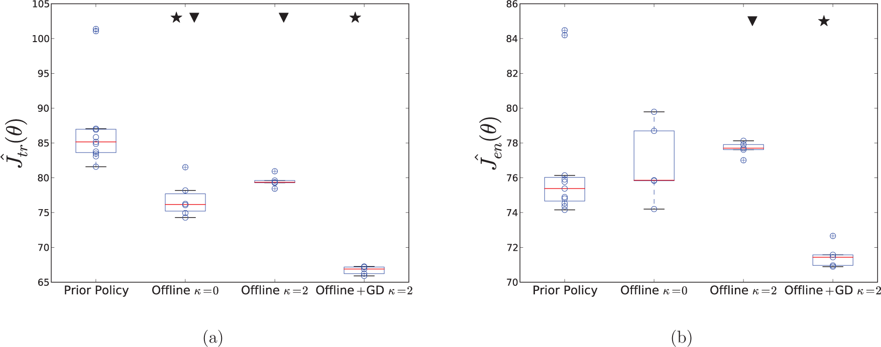
Data from test runs of the prior learned policy, the offline selected risk-neutral and risk-averse policies, and the policy after five episodes of risk-averse gradient descent starting from the risk-averse offline policy: (a) translation aversion; (b) energy aversion. A star at the top of a column signifies a statistically significant reduction in the mean compared with the previous column (Behrens–Fisher, p < 0.01) and a triangle signifies a significant reduction in the variance (F-test, p < 0.03).

For the energy-averse case, the offline risk-neutral policy had no statistically significant difference in sample average or variance compared with the prior learned policy. The risk-averse policy had slightly (not statistically significantly) higher average cost than both the original learned policy and the offline risk-neutral policy, but it had significantly lower variance. The policy learned after five episodes of risk-averse gradient descent had significantly lower average cost than the offline risk-averse while maintaining similar variance (see Figure 11(b)). The statistical significance results given in Figure 11 are strongly in line with our qualitative assessment of the data. However, we should take care to consider these in light of the small sample sizes available, which constrain our ability to verify their underlying assumptions.

6. Related work

Several successful applications of Bayesian optimization to robot control tasks exist in the literature. Lizotte et al. (2007) applied Bayesian optimization to discover an Aibo gait that surpassed the state-of-the-art in a comparatively small number of trials. Tesch et al. (2011) used Bayesian optimization to optimize snake robot gaits in several environmental contexts. Martinez-Cantin et al. (2009) describe an application to online sensing and path planning for mobile robots in uncertain environments. Recently, Kormushev and Caldwell (2012) proposed a particle filter approach for performing direct policy search that is closely related to Bayesian optimization techniques.

A variety of algorithms have been designed to find optimal policies with respect to risk-sensitive criteria. Early work in risk-sensitive control was aimed at extending dynamic programming methods to optimize exponential objective functions. This work included algorithms for solving discrete Markov decision processes (MDPs) (Howard and Matheson, 1972) and linear-quadratic-Gaussian problems (Jacobson, 1973; Whittle, 1981). Borkar derived a variant of the Q-learning algorithm for finite MDPs with exponential utility (Borkar, 2002). Heger (1994) derived a worst-case Q-learning algorithm based on a minimax criterion. For continuous problems, van den Broek et al. (2010) generalized path integral methods from stochastic optimal control to the risk-sensitive case.

Other work has approached the problem of risk-sensitive control with methods other than exponential objective functions. For example, several authors have developed algorithms in discrete model-free RL setting for learning conditional return distributions (Dearden et al., 1998; Morimura et al., 2010a, b), which can be combined with policy selection criteria that take return variance into account. The algorithms discussed in this paper are related to this line of work, but they are more directly applicable to systems with continuous state and action spaces. The recent work of Tamar et al. (2012) describes likelihood-ratio policy gradient algorithms appropriate for different types of risk-sensitive criteria. The simulation-based algorithm in their work is closely related to the RSSGD update rule. However, rather than learning a non-parametric cost model, their algorithm uses a two-timescale approach to obtain incremental unbiased estimates of the cost mean and variance. In some cases, this unbiasedness might be more important than the sample efficiency that cost-model-based approaches can offer.

Policy gradient approaches that are designed to learn dynamic transition models, such as PILCO (Deisenroth and Rasmussen, 2011), can also be used to capture uncertainty in the cost distribution (Deisenroth, 2010). These approaches are capable of handling high-dimensional policy spaces, whereas the approaches described in this work are only appropriate for low-dimensional policy spaces. However, to achieve this scalability, certain smoothness assumptions must be made about the system dynamics. Furthermore, performing offline optimizations to change risk-sensitivity would be significantly more computationally intensive than the approach presented here.

Mihatsch and Neuneier (2002) developed risk-sensitive variants of TD(0) and Q-learning by allowing the step size in the value function update to be a function of the sign of the temporal difference error. For example, by making the step size for positive errors slightly larger than the step size for negative errors, the value of a particular state and action will tend to be optimistic, yielding a risk-seeking system. Recently, this algorithm was found to be consistent with behavioral and neurological measurements taken while humans learned a decision task involving risky outcomes (Niv et al., 2012), suggesting that some form of risk-sensitive TD may be present in the brain.

The connection between these types of methods and biological learning and control processes is an active area of research in the biological sciences. For example, some neuroscience researchers have identified separate neural encodings for expected cost and cost variance that appear to be involved in risk-sensitive decision making (Tobler et al., 2007; Preuschoff et al., 2008). Recent motor control experiments suggest that humans select motor strategies in a risk-sensitive way (Wu et al., 2009; Nagengast et al., 2010a, 2011). For example, Nagengast et al. (2010a) show that control gains selected by human subjects in a noisy control task are consistent with risk-averse optimal control solutions. There is also an extensive literature on risk-sensitive foraging behaviors in a wide variety of species (Kacelnik and Bateson, 1996; Bateson, 2002; Niv et al., 2002).

7. Discussion and future work

In many real-world control problems, it can be advantageous to adjust risk-sensitivity based on runtime context. For example, systems whose environments change in ways that make failures more or less costly (such as operating around catastrophic obstacles or in a safety harness) or when the context demands that the system seek low-probability high-performance events. Perhaps not surprisingly, this variable risk property has been observed in a variety of animal species, from simple motor tasks in humans to foraging birds and bees (Bateson, 2002; Braun et al., 2011).

However, most methods for learning policies by interaction focus on the risk-neutral minimization of expected cost. Extending Bayesian optimization methods to capture policy-dependent cost variance creates the opportunity to select policies with different risk-sensitivity. Furthermore, the ability to efficiently vary risk-sensitivity offers an advantage over existing model-free risk-sensitive control techniques that require separate optimizations and additional policy executions to produce policies with different risk.

The variable risk property was illustrated in experiments applying VBO to the problem of impact stabilization. After a short period of learning, an empirical comparison of policies selected with different CB criteria confirmed the algorithmic predictions about the relative riskiness of each policy. However, how to set the system’s risk-sensitivity for a particular task remains an important open problem. In particular, we saw that when variance is very large for some policies, risk-seeking optimizations must be done carefully to avoid selecting policies with high variance and poor average performance. Other risk-sensitive policy selection criteria may be less susceptible to such phenomena.

Several properties of VBO should be considered when determining its suitability for a particular problem. First, although the computational complexity is the same as Bayesian optimization, $O (N^{3})$ , the greater flexibility of the VHGP model means that VBO tends to require more initial policy evaluations than standard Bayesian optimization. In addition, like many other episodic policy search algorithms, such as Bayesian optimization and finite-difference methods (Kohl and Stone, 2004; Roberts and Tedrake, 2009), VBO is sensitive to the number of policy parameters: high-dimensional policies can require many trials to optimize. These algorithms are therefore most effective in problems where low-dimensional policy representations are available, but accurate system models are not. However, there is evidence that policy spaces at least up to 15 dimensions can be efficiently explored with Bayesian optimization if estimates of the GP hyperparameters can be obtained a priori (Lizotte et al., 2007).

Another important consideration is the choice of kernel functions in the GP priors. In this work, we used the anisotropic squared exponential kernel to encode our prior assumptions regarding the smoothness and regularity of the underlying cost function. However, for many problems the underlying cost function is not smooth or regular; it contains flat regions and sharp discontinuities that can be difficult to represent. An interesting direction for future work is the use kernel functions with local support. Kernels that are not invariant to shifts in policy space will be necessary to capture cost surfaces that, e.g., contain both flat regions and regions with large changes in cost. Methods for capturing multimodality of the cost distribution are also important to consider, especially in domains where unobservable differences in initial conditions can lead to qualitatively different outcomes.

One straightforward way to extend VBO would be to consider different policy selection criteria. In particular, multi-step methods that select a sequence of n policy parameters could be valuable in systems with fixed experimental budgets. Osborne et al. have proposed a multi-step criterion in the standard Bayesian optimization setting that has produced promising results (Osborne et al., 2009; Garnett et al., 2010). Other risk-sensitive global optimization algorithms could also be conceived by using other methods to build the heteroscedastic cost model (Tibshirani and Hastie, 1987; Snelson and Ghahramani, 2006; Kersting et al., 2010; Wilson and Ghahramani, 2011). It would be worthwhile to investigate whether these methods are more appropriate for particular problem domains.

The VBO and RSSGD algorithms are connected by their use of a learned heteroscedastic cost model to perform policy search. VBO uses this model to globally select policies, whereas RSSGD uses it as a local critic to descend the gradient of a risk-sensitive objective. Both algorithms have the advantage of being independent of the dynamics, dimensionality, and cost function structure, and the disadvantage of their performance being dependent on the dimensionality of the policy parameter space. We considered the possibility of interweaving gradient descent with local offline policy selection in dynamic lifting experiments with the uBot-5. First, a policy was learned that exploited the system dynamics to produce an efficient and reliable lifting strategy. Then, starting from this learned policy, new local cost models were fit and used to select translation-averse and energy-averse policies. It is noteworthy that this kind of flexibility is possible after so few trials, especially given the generality of the optimization procedure. However, a limitation of the implementation described is that generalization to different objects or lifting scenarios would require separate optimizations. The extent to which more sophisticated closed-loop or model-based policy representations could support generalization is an interesting open question.

The use of the cost model in the RSSGD algorithm is somewhat restricted and there are several possibilities for improvements. For example, some work has shown that adjusting the covariance of the perturbation distribution while learning can produce better performance (Roberts and Tedrake, 2009). This idea is related to the covariance matrix adaptation that is done in some cost weighted averaging methods (Stulp and Sigaud, 2012). An interesting direction for future work would be to use the learned local model to adjust the sampling distribution by, e.g., scaling the perturbation covariance by the optimized length-scale hyperparameters of the VHGP model. In this way, parameters would be perturbed based on the inferred relative sensitivity of the cost to changes in each parameter value. Methods for using gradient estimates from the local critic to update the policy parameters or, conversely, using gradient observations to update the critic could also be explored.

8. Conclusion

Varying risk-sensitivity based on the runtime context is a potentially powerful way to generate flexible control in robot systems. We considered this problem in the context of model-free policy search, where risk-sensitive parameterized policies can be selected based on a learned cost distribution. Our experimental results suggest that VBO and RSSGD are efficient and plausible methods for achieving variable risk control.

Footnotes

Notes

Funding

Scott Kuindersma was supported by a NASA GSRP Fellowship from Johnson Space Center. Roderic Grupen was supported by the ONR (MURI award N00014-07-1-0749). Andrew Barto was supported by the AFOSR (grant number FA9550-08-1-0418).

References

Abramowitz

Stegun

(eds.) (1972) Handbook of Mathematical Functions with Formulas, Graphs, and Mathematical Tables, 9th printing. New York: Dover.

Amari

(1998) Natural gradient works efficiently in learning. Neural Computation 10(2): 251–276.

Bateson

(2002) Recent advances in our understanding of risk-sensitive foraging preferences. Proceedings of the Nutrition Society 61: 1–8.

Bertsekas

Tsitsiklis

(2000) Gradient convergence in gradient methods with errors. SIAM Journal of Optimization 10(3): 627–642.

Borkar

(2002) Q-learning for risk-sensitive control. Mathematics of Operations Research 27(2): 294–311.

Braun

Nagengast

Wolpert

(2011) Risk-sensitivity in sensorimotor control. Frontiers in Human Neuroscience 5: 1–10.

Brochu

Cora

de Freitas

(2009) A Tutorial on Bayesian Optimization of Expensive Cost Functions, with Application to Active User Modeling and Hierarchical Reinforcement Learning. Technical Report TR-2009-023, University of British Columbia, Department of Computer Science.

Bull

(2011) Convergence rates of efficient global optimization algorithms. Journal of Machine Learning Research 12: 2879–2904.

Cox

John

(1992) A statistical method for global optimization. In: IEEE International Conference on Systems, Man and Cybernetics, 1992, vol. 2, pp. 1241–1246. DOI: 10.1109/ICSMC.1992.271617.

10.

Craig

(2005) Introduction to Robotics: Mechanics and Control, 3rd edition. Pearson Prentice Hall.

11.

Dearden

Friedman

Russell

(1998) Bayesian Q-learning. In: Proceedings of the Fifteenth National Conference on Artificial Intelligence, pp. 761–768.

12.

Deegan

(2010) Whole-Body Strategies for Mobility and Manipulation. PhD thesis, University of Massachusetts Amherst.

13.

Deisenroth

(2010) Efficient Reinforcement Learning using Gaussian Processes. PhD thesis, Karlsruhe Institute of Technology.

14.

Deisenroth

Rasmussen

(2011) PILCO: A model-based and data-efficient approach to policy search. In: Proceedings of the 28th International Conference on Machine Learning, Bellevue, WA.

15.

Frean

Boyle

(2008) Using Gaussian processes to optimize expensive functions. In: AI 2008: Advances in Artificial Intelligence, pp. 258–267.

16.

Garnett

Osborne

Roberts

(2010) Bayesian optimization for sensor set selection. In: Proceedings of the 9th ACM/IEEE International Conference on Information Processing in Sensor Networks. New York: ACM Press, pp. 209–219.

17.

Goldberg

Williams

CKI

Bishop

(1998) Regression with input-dependent noise: A Gaussian process treatment. In: Advances in Neural Information Processing Systems 10 (NIPS), pp. 493–499.

18.

Heger

(1994) Consideration of risk in reinforcement learning. In: Proceedings of the 11th International Conference on Machine Learning (ICML), pp. 105–111.

19.

Howard

Matheson

(1972) Risk-sensitive Markov decision processes. Management Science 18(2): 356–369.

20.

Jabri

Flower

(1992) Weight perturbation: An optimal architecture and learning technique for analog VLSI feedforward and recurrent multi-layer networks. IEEE Transactions on Neural Networks 3: 154–157.

21.

Jacobson

(1973) Optimal stochastic linear systems with exponential performance criteria and their relationship to deterministic differential games. IEEE Transactions on Automatic Control 18(2): 124–131.

22.

Johnson

(2011) The NLopt nonlinear-optimization package. http://ab-initio.mit.edu/nlopt.

23.

Jones

(2001) A taxonomy of global optimization methods based on response surfaces. Journal of Global Optimization 21: 345–383.

24.

Kacelnik

Bateson

(1996) Risky theories—the effects of variance on foraging decisions. American Zoologist 36: 402–434.

25.

Kakade

(2002) A natural policy gradient. In: Advances in Neural Information Processing Systems 14 (NIPS).

26.

Kersting

Plagemann

Pfaff

Burgard

(2010) Most likely heteroscedastic Gaussian process regression. In: Proceedings of the International Conference on Machine Learning (ICML), pp. 393–400.

27.

Kober

Peters

(2009) Policy search for motor primitives in robotics. In: Advances in Neural Information Processing Systems 21. Cambridge, MA: MIT Press.

28.

Kohl

Stone

(2004) Machine learning for fast quadrupedal locomotion. In: Proceedings of the Nineteenth National Conference on Artificial Intelligence, pp. 611–616.

29.

Kolter

(2010) Policy search via the signed derivative. In: Robotics: Science and Systems V (RSS).

30.

Kormushev

Caldwell

(2012) Direct policy search reinforcement learning based on particle filtering. In: Proceedings of the 10th European Workshop on Reinforcement Learning.

31.

Kuindersma

Grupen

Barto

(2011) Learning dynamic arm motions for postural recovery. In: Proceedings of the 11th IEEE-RAS International Conference on Humanoid Robots, Bled, Slovenia, pp. 7–12.

32.

Kuindersma

Grupen

Barto

(2012a) Variable risk dynamic mobile manipulation. In: RSS 2012 Workshop on Mobile Manipulation, Sydney, Australia.

33.

Kuindersma

Grupen

Barto

(2012b) Variational Bayesian optimization for runtime risk-sensitive control. In: Robotics: Science and Systems VIII (RSS), Sydney, Australia.

34.

Kuindersma

Hannigan

Ruiken

Grupen

(2009) Dexterous mobility with the uBot-5 mobile manipulator. In: Proceedings of the 14th International Conference on Advanced Robotics, Munich, Germany.

35.

Kushner

(1964) A new method of locating the maximum of an arbitrary multipeak curve in the presence of noise. Journal of Basic Engineering 86: 97–106.

36.

Lázaro-Gredilla

Titsias

(2011) Variational heteroscedastic Gaussian process regression. In: Proceedings of the International Conference on Machine Learning (ICML).

37.

Levy

Markowitz

(1979) Approximating expected utility by a function of mean and variance. The American Economic Review 69(3): 308–317.

38.

Lizotte

Wang

Bowling

Schuurmans

(2007) Automatic gait optimization with Gaussian process regression. In: Proceedings of the Twentieth International Joint Conference on Artificial Intelligence (IJCAI).

39.

Lizotte

Greiner

Schuurmans

(2011) An experimental methodology for response surface optimization methods. Journal of Global Optimization 53(4): 699–736.

40.

Martinez-Cantin

de Freitas

Brochu

Castellanos

Doucet

(2009) A Bayesian exploration-exploitation approach for optimal online sensing and planning with a visually guided mobile robot. Autonomous Robots 27: 93–103.

41.

Martinez-Cantin

de Freitas

Doucet

Castellanos

(2007) Active policy learning for robot planning and exploration under uncertainty. In: Proceedings of Robotics: Science and Systems.

42.

Mihatsch

Neuneier

(2002) Risk-sensitive reinforcement learning. Machine Learning 49: 267–290.

43.

Morimura

Sugiyama

Kashima

Hachiya

(2010a) Nonparametric return distribution approximiation for reinforcement learning. In: Proceedings of the 27th International Conference on Machine Learning (ICML).

44.

Morimura

Sugiyama

Kashima

Hachiya

Tanaka

(2010b) Parametric return density estimation for reinforcement learning. In: Proceedings of the 26th Conference on Uncertainty in Artificial Intelligence (UAI 2010).

45.

Močckus

Tiesis

Žilinskas

(1978) The application of Bayesian methods for seeking the extremum. In: Toward Global Optimization, volume 2. Amsterdam: Elsevier, pp. 117–128.

46.

Nagengast

Braun

Wolpert

(2010a) Risk-sensitive optimal feedback control accounts for sensorimotor behavior under uncertainty. PLoS Computational Biology 6(7): 1–15.

47.

Nagengast

Braun

Wolpert

(2011) Risk-sensitivity and the mean-variance trade-off: decision making in sensorimotor control. Proceedings of the Royal Society B 278(1716): 2325–2332.

48.

Niv

Edlund

Dayan

O’Doherty

(2012) Neural prediction errors reveal a risk-sensitive reinforcement-learning process in the human brain. Journal of Neuroscience 32(2): 551–562.

49.

Niv

Joel

Meilijson

Ruppin

(2002) Evolution of reinforcement learning in uncertain environments: A simple explanation for complex foraging behaviors. Adaptive Behavior 10(1): 5–24.

50.

Osborne

Garnett

Roberts

(2009) Gaussian processes for global optimization. In: Third International Conference on Learning and Intelligent Optimization (LION3), Trento, Italy.

51.

Peters

Schaal

(2006) Policy gradient methods for robotics. In: Proceedings of the IEEE International Conference on Intelligent Robots and Systems (IROS), pp. 2219–2225.

52.

Preuschoff

Quartz

Bossaerts

(2008) Human insula activation reflects risk prediction errors as well as risk. Journal of Neuroscience 28(11): 2745–2752.

53.

Rasmussen

Williams

CKI

(2006) Gaussian Processes for Machine Learning. Cambridge, MA: MIT Press.

54.

Roberts

Moret

Zhang

Tedrake

(2010) Motor learning at intermediate Reynolds number: experiments with policy gradient on the flapping flight of a rigid wing. In: Sigaud

Peters

(eds.) From Motor to Interaction Learning in Robots (Studies in Computational Intelligence, vol. 264). Berlin: Springer, pp. 293–309.

55.

Roberts

Tedrake

(2009) Signal-to-noise ratio analysis of policy gradient algorithms. In: Advances of Neural Information Processing Systems 21 (NIPS).

56.

Rosenstein

Barto

(2001) Robot weightlifting by direct policy search. In: Proceedings of the International Joint Conference on Artificial Intelligence (IJCAI).

57.

Schonlau

Welch

Jones

(1998) Global versus local search in constrained optimization of computer models. In: Flournoy

Rosenberger

Wong

(eds.) New Developments and Applications in Experimental Design (Lecture Notes - Monograph Series, vol. 34). IMS, pp. 11–25.

58.

Sharpe

(1966) Mutual fund performance. Journal of Business 39(S1): 119–138.

59.

Snelson

Ghahramani

(2006) Variable noise and dimensionality reduction for sparse Gaussian processes. In: Proceedings of the 22nd Conference on Uncertainty in Artificial Intelligence, Cambridge, MA.

60.

Srinivas

Krause

Kakade

Seeger

(2010) Gaussian process optimization in the bandit setting: No regret and experimental design. In: Proceedings of the 27th International Conference on Machine Learning (ICML).

61.

Stulp

Sigaud

(2012) Path integral policy improvement with covariance matrix adaptation. In: Proceedings of the 29th International Conference on Machine Learning (ICML), Edinburgh, Scotland.

62.

Tamar

Castro

Mannor

(2012) Policy gradients with variance related risk criteria. In: Proceedings of the 29th International Conference on Machine Learning (ICML), Edinburgh, Scotland.

63.

Tedrake

Zhang

Seung

(2004) Stochastic policy gradient reinforcement learning on a simple 3D biped. In: Proceedings of the IEEE International Conference on Intelligent Robots and Systems (IROS), volume 3, Sendai, Japan, pp. 2849–2854.

64.

Tesch

Schneider

Choset

(2011) Using response surfaces and expected improvement to optimize snake robot gait parameters. In: Proceedings of the IEEE/RSJ International Conference on Intelligent Robots and Systems (IROS), San Francisco, CA.

65.

Theodorou

Buchli

Schaal

(2010) Reinforcement learning of motor skills in high dimensions: A path integral approach. In: Proceedings of the IEEE International Conference on Robotics and Automation, Anchorage, AK.

66.

Tibshirani

Hastie

(1987) Local likelihood estimation. Journal of the American Statistical Association 82(398): 559–567.

67.

Tobler

O’Doherty

Dolan

Schultz

(2007) Reward value coding distinct from risk attitude-related uncertainty coding in human reward systems. Journal of Neurophysiology 97: 1621–1632.

68.

van den Broek

Wiegerinck

Kappen

(2010) Risk sensitive path integral control. In: Proceedings of the 26th Conference on Uncertainty in Artificial Intelligence (UAI), pp. 615–622.

69.

Vazquez

Bect

(2010) Convergence properties of the expected improvement algorithm with fixed mean and covariance functions. Journal of Statistical Planing and Inference 140(11): 3088–3095.

70.

Whittle

(1981) Risk-sensitive linear/quadratic/Gaussian control. Advances in Applied Probability 13: 764–777.

71.

Whittle

(1990) Risk-Sensitive Optimal Control. New York: John Wiley & Sons.

72.

Williams

(1992) Simple statistical gradient-following algorithms for connectionist reinforcement learning. Machine Learning 8: 229–256.

73.

Wilson

Fern

Tadepalli

(2011) A behavior based kernel for policy search via Bayesian optimization. In: Proceedings of the ICML 2011 Workshop: Planning and Acting with Uncertain Model, Bellevue, WA.

74.

Wilson

Ghahramani

(2011) Generalized Wishart processes. In: Proceedings of the 27th Conference on Uncertainty in Artificial Intelligence (UAI), Barcelona, Spain.

75.

Delgado

Maloney

(2009) Economic decision-making compared with an equivalent motor task. Proceedings of the National Academy of Sciences of the USA 106(15): 6088–6093.